Abstract
AbstractThree-dimensional (3D) reconstructions from electron tomography provide important morphological, compositional, optical and electro-magnetic information across a wide range of materials and devices. Precession electron diffraction, in combination with scanning transmission electron microscopy, can be used to elucidate the local orientation of crystalline materials. Here we show, using the example of a Ni-base superalloy, that combining these techniques and extending them to three dimensions, to produce scanning precession electron tomography, enables the 3D orientation of nanoscale sub-volumes to be determined and provides a one-to-one correspondence between 3D real space and 3D reciprocal space for almost any polycrystalline or multi-phase material.
🔬 Techniques
🔭 Microscopes
🏭 Microscope Brands
📷 Detectors
💻 Software Details
🏛️ Research Organizations (ROR)
Affiliated research institutions:
📋 Methods
Electron microscopy experiments
SPED was performed on a Philips CM300 FEGTEM operating at 300 kV. The scan and precession were controlled through a Nanomegas Digistar connected to the microscope and running the ASTAR software package. For the experiments, a small-angle convergent probe (convergence semiangle of 1.4 mrad) was used to allow the separation of closely spaced reflections (expected for the η-phase). Source size demagnification (first condenser lens strength) was modest to retain a high beam current to facilitate short exposure times at the expense of a larger probe size. A relatively small precession angle of 0.5° (8.7 mrad) was chosen to increase sufficiently the number of reflections detected in each diffraction pattern, and hence increase the reliability of indexing, but not to lead to excessive beam-broadening through the specimen volume 10 . We estimate the final probe size was 5 nm in diameter. Each scan was 120 × 120 pixels 2 with pixel steps of 7.5 nm and a PED pattern recorded at each point, patterns were recorded using a Stingray CCD camera, which captures the image on the binocular viewing screen. The recorded image was corrected for geometric distortion before crystallographic analysis. The precession frequency was 100 Hz and the dwell time at each pixel was 20 ms to ensure complete integration around the precession circle. The sample was tilted at 5° intervals from −60° to +70° using a Fischione 2020 tomography holder.
Statistical decomposition Non-negative matrix factorization
(NMF) was performed using the ‘Hyperspy' software package. Each SPED data set was loaded as a stack of 14,400 diffraction patterns (from the 120 × 120 pixel 2 scan). NMF decomposition of the image stack was performed assuming Poisson noise and for a range of expected components. Through trial-and-error, a total of 20 components was found to return results that reliably matched features we were able to identify for each of the major phases (matrix, carbide and η-phase) in the sample while minimizing the calculation time. Examples are shown in Fig. 1 . NMF constrains both the components and the loadings to be positive, as a reasonable a priori constraint and in the hope that both may then be physically interpretable: the component patterns resemble conventional diffraction patterns and the loading maps virtual dark-field (VDF) images. By decomposing the data using NMF, the component patterns can be used directly as input for the reciprocal lattice reconstruction and the loadings as images for real space reconstruction. As an example, the component patterns and loading maps, associated with the facetted metal carbide particle across the tilt series, are shown in Supplementary Fig. 1 . The loading maps have been binarized to simplify the image input for the geometric tomographic reconstruction of the carbide particle—to produce a 3D ‘envelope'. The results from +30° to +45° were corrupted by shadowing from a piece of carbon film and are not used in the analysis. A second component pattern/loading pair was associated with the carbide, another with the η phase and the remaining 17 component/loading pairs associated with the matrix. The large number reflects the complex orientation changes seen in the matrix brought about by slowly varying tilt, bending and the presence of a low angle boundary within the field of view. Although not of importance here, this indicates the sensitivity of the NMF routine in identifying small orientation changes in strained material. Tomography reconstructions Reconstruction of the real-space volumes from the loading maps of the three phases was undertaken using FEI Inspect3D software. Volume rendering was achieved using the Avizo Fire software package. Reconstruction of the reciprocal lattice for each component was performed using in-house software. Crystal structure determination The f.c.c. crystal structure of the matrix was confirmed by analysis of the and projections of the reconstructed 3D reciprocal lattice, as shown in Supplementary Fig. 2a and b , respectively. The zero-order Laue zone (ZOLZ) reflections were identified by analysing a central slice (containing the origin) of the reconstruction normal to the viewing direction. As the tilt series is not complete (missing wedge of information), the ZOLZ was only partially sampled in the central slice. However, by using auto-correlation, the ZOLZ geometry was improved greatly, see coloured overlay of spots. From these two projections, a body-centred reciprocal lattice is evident, confirming an f.c.c. real-space lattice. Using the internal ASTAR calibration values (0.604 mrad per pixel, an effective camera length of 126mm), the lattice parameter for the matrix was determined to be 3.60 Å+/−0.06 Å, which agrees well with the expected value for the γ-phase in a nickel-base superalloy 29 . The error was estimated by considering the variation in orientation of the reciprocal lattice. Given the possibility of up to 0.5° error in the tilt axis measurement, combined (in quadrature) with the cluster size of ∼0.2° around each reciprocal lattice point, the aligned sample was mis-tilted by 0.54° in eight randomly determined directions. Each of the eight reconstructed reciprocal lattices underwent the same autocorrelation and geometric analysis to determine the cell parameters. The mean and s.d. of these parameters are the reported values. In the same way, the reconstructed 3D reciprocal lattice of the metal carbide was oriented along the and zone axes, as shown in Supplementary Fig. 2c and d , respectively. Although the number of reflections uniquely assigned to the carbide is fewer than that of the matrix, with a somewhat noisier reconstruction as a result, the figures still clearly show reciprocal space projections consistent with a f.c.c structure. The measured lattice parameter of 4.43+/−0.07 Å is consistent with (Nb/Ti)C 29 , with the NaCl structure, known to exist in this superalloy. Ti and Nb are both strong carbide forming elements in this alloy system and the corresponding carbide lattice parameters vary, depending on the non-stoichiometry of the carbon, between 4.33 Å and 4.27 Å for TiC and 4.47 Å and 4.42 Å for NbC, respectively. Composition of the metal carbide Chemical mapping of the region of interest was performed on an FEI Tecnai Osiris (S)TEM, fitted with a large solid-angle silicon drift detector (SDD) for STEM-EDX measurements. A summary of the results are shown in Supplementary Fig. 3 . The upper half of the figure shows element maps formed from the K peaks of the expected alloy elements, the lower half shows the integrated EDX spectrum for the central portion of the facetted particle. The Nb signal is clearly strongest in this region and, together with the large Nb:Ti ratio in the EDX spectrum, confirms the particle is Nb-rich. Crystal orientation determination The structure analysis was confirmed by inspection of the output from pattern fitting (software provided as part of the ASTAR system) between structure libraries (generated with the measured lattice parameters listed above) and the component patterns returned by the decomposition. The comparison of the component pattern (P) with the template library of patterns (T) is quantified using a Correlation Index (Q) 35 : Supplementary Fig. 4a shows and example of a match between the best fit in the pattern library (as a coloured overlay) for the component pattern corresponding to the matrix at a tilt of −5°. The orientation is confirmed in Supplementary Fig. 4b that shows the Correlation Index for all of the unique patterns in the library as a function of their position in the stereographic triangle (a symmetry independent sector of reciprocal space for the f.c.c. crystal). For the figure, the lower the value of Q the poorer the match and this is assigned a light tone, the higher values of Q (better fits) are assigned a darker tone; the position of the best fit is indicated with a coloured dot. The same analysis is shown for the carbide component in Supplementary Fig. 4c and 4d , respectively. The stereographic pole figures were produced using the MTEX package for MATLAB. Matrix strain and composition near the carbide The elemental maps in Supplementary Fig. 4 show the presence of the fine-scale γ' particles, rich in nickel and aluminium/titanium (γ' is based around the ordered Ni 3 Ti or Ni 3 Al structure) and the corresponding absence of the other elements (iron, chromium and cobalt). These other elements, together with oxygen, are present throughout the matrix but appear to be enhanced in the region of the carbide. One of the 17 component patterns associated with the matrix is shown in Supplementary Fig. 5a , together with its corresponding loading in 5b. Although at first glance the loading map appears to be indicating the carbide, the component pattern can be indexed only as one associated with the matrix phase. Thus, the loading map must be associated with a region of matrix above and/or below the carbide. Moreover, the strong contrast seen in the loading map matches the EDX elemental map contrast for all the elements except Ni and Ti (which are preferentially in the carbide). The best match for the component pattern in Supplementary Fig. 5a is, however, found when the matrix is strained isotropically in a tensile manner by 3.1%, qualitatively consistent with the strain needed to achieve the CSL seen in Fig. 4 . The heterogeneous solute segregation in the matrix near the carbide, identified in the EDX elemental maps, may also be driven by strain at the carbide/matrix interface.
Show full methods section
Electron microscopy experiments
SPED was performed on a Philips CM300 FEGTEM operating at 300 kV. The scan and precession were controlled through a Nanomegas Digistar connected to the microscope and running the ASTAR software package. For the experiments, a small-angle convergent probe (convergence semiangle of 1.4 mrad) was used to allow the separation of closely spaced reflections (expected for the η-phase). Source size demagnification (first condenser lens strength) was modest to retain a high beam current to facilitate short exposure times at the expense of a larger probe size. A relatively small precession angle of 0.5° (8.7 mrad) was chosen to increase sufficiently the number of reflections detected in each diffraction pattern, and hence increase the reliability of indexing, but not to lead to excessive beam-broadening through the specimen volume 10 . We estimate the final probe size was 5 nm in diameter. Each scan was 120 × 120 pixels 2 with pixel steps of 7.5 nm and a PED pattern recorded at each point, patterns were recorded using a Stingray CCD camera, which captures the image on the binocular viewing screen. The recorded image was corrected for geometric distortion before crystallographic analysis. The precession frequency was 100 Hz and the dwell time at each pixel was 20 ms to ensure complete integration around the precession circle. The sample was tilted at 5° intervals from −60° to +70° using a Fischione 2020 tomography holder.
Statistical decomposition Non-negative matrix factorization
(NMF) was performed using the ‘Hyperspy' software package. Each SPED data set was loaded as a stack of 14,400 diffraction patterns (from the 120 × 120 pixel 2 scan). NMF decomposition of the image stack was performed assuming Poisson noise and for a range of expected components. Through trial-and-error, a total of 20 components was found to return results that reliably matched features we were able to identify for each of the major phases (matrix, carbide and η-phase) in the sample while minimizing the calculation time. Examples are shown in Fig. 1 . NMF constrains both the components and the loadings to be positive, as a reasonable a priori constraint and in the hope that both may then be physically interpretable: the component patterns resemble conventional diffraction patterns and the loading maps virtual dark-field (VDF) images. By decomposing the data using NMF, the component patterns can be used directly as input for the reciprocal lattice reconstruction and the loadings as images for real space reconstruction. As an example, the component patterns and loading maps, associated with the facetted metal carbide particle across the tilt series, are shown in Supplementary Fig. 1 . The loading maps have been binarized to simplify the image input for the geometric tomographic reconstruction of the carbide particle—to produce a 3D ‘envelope'. The results from +30° to +45° were corrupted by shadowing from a piece of carbon film and are not used in the analysis. A second component pattern/loading pair was associated with the carbide, another with the η phase and the remaining 17 component/loading pairs associated with the matrix. The large number reflects the complex orientation changes seen in the matrix brought about by slowly varying tilt, bending and the presence of a low angle boundary within the field of view. Although not of importance here, this indicates the sensitivity of the NMF routine in identifying small orientation changes in strained material. Tomography reconstructions Reconstruction of the real-space volumes from the loading maps of the three phases was undertaken using FEI Inspect3D software. Volume rendering was achieved using the Avizo Fire software package. Reconstruction of the reciprocal lattice for each component was performed using in-house software. Crystal structure determination The f.c.c. crystal structure of the matrix was confirmed by analysis of the and projections of the reconstructed 3D reciprocal lattice, as shown in Supplementary Fig. 2a and b , respectively. The zero-order Laue zone (ZOLZ) reflections were identified by analysing a central slice (containing the origin) of the reconstruction normal to the viewing direction. As the tilt series is not complete (missing wedge of information), the ZOLZ was only partially sampled in the central slice. However, by using auto-correlation, the ZOLZ geometry was improved greatly, see coloured overlay of spots. From these two projections, a body-centred reciprocal lattice is evident, confirming an f.c.c. real-space lattice. Using the internal ASTAR calibration values (0.604 mrad per pixel, an effective camera length of 126mm), the lattice parameter for the matrix was determined to be 3.60 Å+/−0.06 Å, which agrees well with the expected value for the γ-phase in a nickel-base superalloy 29 . The error was estimated by considering the variation in orientation of the reciprocal lattice. Given the possibility of up to 0.5° error in the tilt axis measurement, combined (in quadrature) with the cluster size of ∼0.2° around each reciprocal lattice point, the aligned sample was mis-tilted by 0.54° in eight randomly determined directions. Each of the eight reconstructed reciprocal lattices underwent the same autocorrelation and geometric analysis to determine the cell parameters. The mean and s.d. of these parameters are the reported values. In the same way, the reconstructed 3D reciprocal lattice of the metal carbide was oriented along the and zone axes, as shown in Supplementary Fig. 2c and d , respectively. Although the number of reflections uniquely assigned to the carbide is fewer than that of the matrix, with a somewhat noisier reconstruction as a result, the figures still clearly show reciprocal space projections consistent with a f.c.c structure. The measured lattice parameter of 4.43+/−0.07 Å is consistent with (Nb/Ti)C 29 , with the NaCl structure, known to exist in this superalloy. Ti and Nb are both strong carbide forming elements in this alloy system and the corresponding carbide lattice parameters vary, depending on the non-stoichiometry of the carbon, between 4.33 Å and 4.27 Å for TiC and 4.47 Å and 4.42 Å for NbC, respectively. Composition of the metal carbide Chemical mapping of the region of interest was performed on an FEI Tecnai Osiris (S)TEM, fitted with a large solid-angle silicon drift detector (SDD) for STEM-EDX measurements. A summary of the results are shown in Supplementary Fig. 3 . The upper half of the figure shows element maps formed from the K peaks of the expected alloy elements, the lower half shows the integrated EDX spectrum for the central portion of the facetted particle. The Nb signal is clearly strongest in this region and, together with the large Nb:Ti ratio in the EDX spectrum, confirms the particle is Nb-rich. Crystal orientation determination The structure analysis was confirmed by inspection of the output from pattern fitting (software provided as part of the ASTAR system) between structure libraries (generated with the measured lattice parameters listed above) and the component patterns returned by the decomposition. The comparison of the component pattern (P) with the template library of patterns (T) is quantified using a Correlation Index (Q) 35 : Supplementary Fig. 4a shows and example of a match between the best fit in the pattern library (as a coloured overlay) for the component pattern corresponding to the matrix at a tilt of −5°. The orientation is confirmed in Supplementary Fig. 4b that shows the Correlation Index for all of the unique patterns in the library as a function of their position in the stereographic triangle (a symmetry independent sector of reciprocal space for the f.c.c. crystal). For the figure, the lower the value of Q the poorer the match and this is assigned a light tone, the higher values of Q (better fits) are assigned a darker tone; the position of the best fit is indicated with a coloured dot. The same analysis is shown for the carbide component in Supplementary Fig. 4c and 4d , respectively. The stereographic pole figures were produced using the MTEX package for MATLAB. Matrix strain and composition near the carbide The elemental maps in Supplementary Fig. 4 show the presence of the fine-scale γ' particles, rich in nickel and aluminium/titanium (γ' is based around the ordered Ni 3 Ti or Ni 3 Al structure) and the corresponding absence of the other elements (iron, chromium and cobalt). These other elements, together with oxygen, are present throughout the matrix but appear to be enhanced in the region of the carbide. One of the 17 component patterns associated with the matrix is shown in Supplementary Fig. 5a , together with its corresponding loading in 5b. Although at first glance the loading map appears to be indicating the carbide, the component pattern can be indexed only as one associated with the matrix phase. Thus, the loading map must be associated with a region of matrix above and/or below the carbide. Moreover, the strong contrast seen in the loading map matches the EDX elemental map contrast for all the elements except Ni and Ti (which are preferentially in the carbide). The best match for the component pattern in Supplementary Fig. 5a is, however, found when the matrix is strained isotropically in a tensile manner by 3.1%, qualitatively consistent with the strain needed to achieve the CSL seen in Fig. 4 . The heterogeneous solute segregation in the matrix near the carbide, identified in the EDX elemental maps, may also be driven by strain at the carbide/matrix interface.
Data availability
All relevant data present in this publication can be accessed at http://www.repository.cam.ac.uk/handle/1810/247679 .
Supplementary Material Supplementary Information Supplementary Figures 1-5 Supplementary Movie 1 This movie shows the rotation of the volume reconstruction of the carbide particle (left) and the reciprocal lattice reconstructions of the carbide (centre) and the matrix (right). The initial position of all three reconstructions is set to the 0° tilt position in the tilt-series and in all cases the tilt-axis is oriented vertically. An indexed autocorrelation of the reciprocal lattice is overlaid to show the orientation of each phase.
📊 Figures
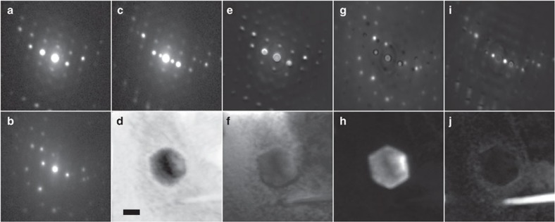
Figure 1
SPED data from the nickel superalloy sample.
Representative PED patterns corresponding to ( a ) the matrix phase (u03b3), ( b ) a metal carbide precipitate and ( c ) a u03b7-phase lath-like precipitate. ( d ) A virtual bright-field image of the ...
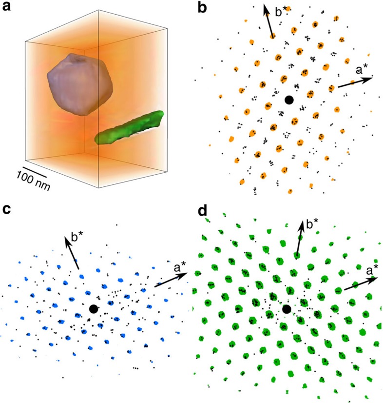
Figure 2
Real space and reciprocal space reconstructions of the Ni-base superalloy microstructure.
( a ) 3D reconstruction of the superalloy volume showing the faceted metal carbide (blue), the u03b7-phase (green) and the surrounding matrix phase (orange). Scale bar, 100u2009nm. [001] zone axis pro...
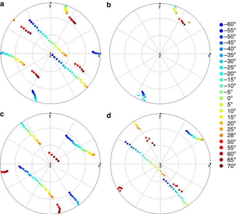
Figure 3
Pole figures showing the orientation of the phases in the tilt-series.
( a , b ) show pole-figures representing the {111} zone axes of the u03b3-matrix and the [0001] zone axis of the u03b7-phase, respectively. The orientation at each step of the tilt series is plotted f...
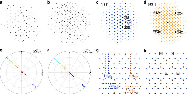
Figure 4
Orientation and structural information from the interface between the matrix and the metal carbide particle.
( a , b ) show the 3D reciprocal lattice reconstruction for the metal carbide and matrix, respectively, projected parallel to the normal of the large facet of the carbide particle, approximately the o...
Figure images are served from the NIH/NLM PubMed Central Open Access Subset or Europe PMC; copyright remains with the publishers and authors.
💬 Discussion
0 commentsNo comments yet. Be the first to start a discussion!
Leave a Comment