Abstract
Persistent neural activity in cortical, hippocampal, and motor networks has been described as mediating working memory for transiently encountered stimuli1,2. Internal emotional states, such as fear, also persist following exposure to an inciting stimulus3, but it is unclear whether slow neural dynamics are involved in this process. Neurons in the dorsomedial and central subdivisions of the ventromedial hypothalamus (VMHdm/c) that express the nuclear receptor protein NR5A1 (also known as SF1) are necessary for defensive responses to predators in mice4-7. Optogenetic activation of these neurons, referred to here as VMHdmSF1 neurons, elicits defensive behaviours that outlast stimulation5,8, which suggests the induction of a persistent internal state of fear or anxiety. Here we show that in response to naturalistic threatening stimuli, VMHdmSF1 neurons in mice exhibit activity that lasts for many tens of seconds. This persistent activity was correlated with, and required for, persistent defensive behaviour in an open-field assay, and depended on neurotransmitter release from VMHdmSF1 neurons. Stimulation and calcium imaging in acute slices showed that there is local excitatory connectivity between VMHdmSF1 neurons. Microendoscopic calcium imaging of VMHdmSF1 neurons revealed that persistent activity at the population level reflects heterogeneous dynamics among individual cells. Unexpectedly, distinct but overlapping VMHdmSF1 subpopulations were persistently activated by different modalities of threatening stimulus. Computational modelling suggests that neither recurrent excitation nor slow-acting neuromodulators alone can account for persistent activity that maintains stimulus identity. Our results show that stimulus-specific slow neural dynamics in the hypothalamus, on a time scale orders of magnitude longer than that of working memory in the cortex9,10, contribute to a persistent emotional state.
🔬 Techniques
🔭 Microscopes
✨ Fluorophores
🧪 Sample Preparation
🔬 Cell Lines
🏭 Microscope Brands
🧪 Reagent Suppliers
📷 Detectors
💻 Software Details
💻 Code & Software
📂💾 Data Repositories
🏛️ Research Organizations (ROR)
Affiliated research institutions:
📋 Methods
Anatomical abbreviations. VNO - vomeronasal organ, AOB - accessory olfactory bulb, MeApv –posterioventral medial amygdala, BNSTif – interfascicular part of bed nucleus of the stria terminalis, VMHdm – dorosmedial ventromedial hypothalamus, AHN – anterior hypothalamic nucleus, PMd - dorsal premammillary nucleus, PAG - periaqueductal gray, Thal – thalamus, LA – lateral amygdala, BS – brain stem, BLA – basolateral amygdala, CEA – central amygdala. Animals. All experimental procedures involving the use of live animals or their tissues were performed in accordance with the NIH guidelines and approved by the Institutional Animal Care and Use Committee (IACUC) and the Institutional Biosafety Committee at the California Institute of Technology (Caltech). SF1-Cre mice were obtained from Dr. Brad Lowell 37 and maintained as heterozygotes in the Caltech animal facility as described previously; the SF1-Cre line is also available from the Jackson Laboratory (Stock No: 012462). An account of the specificity of SF1-Cre expression within VMH and characterization of neurons labeled by Cre-expression can be found in 5 . Heterozygous or wild-type littermate male mice, aged between 8 to 20 weeks, were used in this study. Because hypothalamic nuclei such as VMH show sexually dimorphic gene expression 38 – 40 , it is possible that the functional role of VMHdm SF1 neurons is sex-specific and that it varies with the estrous cycle. We therefore chose to perform all experiments in male mice, to be consistent with our previous characterization of VMHdm SF1 neurons 5 . The study of VMHdm SF1 function in females is of obvious interest 41 , but requires systematic characterization of the effect of estrous cycle phase on the behavior of interest. All mice were housed in ventilated micro-isolator cages in a temperature- and humidity- controlled environment under a reversed 12-hour dark-light cycle, and had free access to food and water. Mouse cages were changed weekly on a fixed day on which experiments were not performed. Long-Evans rats (for use as predators) were obtained from Charles River at 2–3 months of age, and raised to 5–10 months in the Caltech animal facilities. Virus. AAV1.Syn.Flex.GCaMP6s.WPRE.SV40 (CS1113) was obtained from the Penn Vector Core. AAV5.EF1a.DIO.iC++.eYFP and AAV2.EF1a.DIO.hChR2.eYFP.WPRE.pA were obtained from the University of North Carolina Vectors Core. For ex vivo electrophysiology and Ca 2+ imaging studies of VMHdm SF1 neurons, SF1Cre −/ + male mice were injected in VMHdm with 200 nL of of AAV9-Syn-FLEX-jGCaMP7s-WPRE (addgene 104491-AAV9) 5.3 × 10 12 genomic copies per mL and AAV5-Syn-FLEX-rc[ChrimsonR-tdTomato] (addgene 62723-AAV5) 1.1 × 10 12 genomic copies per mL. Surgery. Mice 8–20 weeks old were anesthetized with 5% isoflurane and mounted in a stereotaxic apparatus (Kopf Instruments). 1% - 1.5% isoflurane was used to maintain the anesthesia throughout the surgery procedure. An incision was made to exposure the skull and small craniotomies were made dorsal to each injection site with a stereotaxic mounted drill. Virus suspension (~600 nl) was injected to the VMHdm/c (ML +/− 0.5, AP −4.65, DV −5.6) at a rate of 60 nl/minute using a pulled glass capillary (~40 μm inner diameter at tip) mounted in a nanoliter injector (Nanoliter 2000, World Precision Instruments) controlled by a four channel micro controller (Micro4, World Precision Instruments). Capillaries were kept in place for 10 minutes following injections to allow the adequate diffusion of virus solution and to reduce the virus backflow during capillary withdraw. For fiber photometry, a custom-made unilateral fiber cannula (400 μm in core diameter, 0.48 NA, Doric Lenses) was implanted after virus injection (ML +/−0.4, AP −4.65, DV −5.4). Metabond (Parkell) and dental cement (Bosworth) were applied to secure the implanted ferrule and cover the exposed skull. For optogenetics, a custom-made bilateral fiber cannula aimed 500 μm above each injection site (200 μm in core diameter, 0.37 NA, Doric Lenses) was implanted and held in place with Metabond and dental cement. For in vivo silicon probe recordings, SF1-Cre mice 8–12 weeks old were anesthetized with 5% isoflurane and mounted in a stereotaxic apparatus. 1%−5% isoflurane was used to maintain the anesthesia throughout the surgery. An incision was made to exposure the skull. A craniotomy window (500 um x 500 um, center: ML: +0.3, AP: −4.65) was made on the right hemisphere above the recording site and covered with a thin layer of silicone adhesive compound (WPI) for protection. A custom-made head-bar was leveled and attached to the skull using Metabond. Another small craniotomy was made on the contralateral hemisphere for the insertion of reference wire during recording. Surgery for microendoscopic imaging was performed as previously described 19 . Briefly, we first performed a series of titration experiments of the original viral stock, to determine the virus concentration at which the brightest cytoplasmic but non-nuclear GCaMP6s expression could be observed in slices of fixed brain tissue of the injected mice 4 weeks after injection. The optimal viral dilution was then used to inject mice for in vivo imaging as described above. 2–3 weeks after viral injections, mice were implanted with a graded-index (GRIN) lens (diameter - 0.5 mm, length - 8.4 mm, catalogue #1050–002212, Inscopix) using a supporting device (Proview Implant Kit, cat# 1050–002334, Inscopix). The implantation depth of the lens was determined based on the live visualization of (anesthetized) neural activity as the lens was inserted. Metabond was used to stabilize the lens, and Kwik-Sil sealant (World Precision Instruments) was used to cover the lens surface. After another 2–3 weeks, mice were anesthetized for placement of a microendoscope baseplate (cat# 1050–002192, Inscopix) and a baseplate cover (catalogue #1050–002193, Inscopix) was used to protect the lens when not in use. Five out of twenty implanted animals were selected for in vivo imaging studies based on clarity of cytoplasmic GCaMP6s expression. Stimuli Presentation. Stimuli were presented either in the mouse’s home cage or in a head-fixation set up. In the home cage, a hand-held anesthetized rat weighing 400–600 g was brought in close proximity to the mouse. A stuffed toy rat of approximately the same size as the live rat was used as a control. For the head-fixed preparation, the mouse was placed on a plastic running wheel (15.5 cm diameter) and stabilized by the head-plate (World Precision Instruments, Catalogue #503617) with a custom made tethering system. Animals were habituated to the head-fixation setup for 1 hour each day for 2–3 days before experiments began. Physical stimuli (an awake behaving rat, a conspecific BALB/6 male mouse or a toy rat) were each presented inside a small wire mesh cage, which was held by the experimenter in front of the experimental mouse. Auditory stimuli were presented at 85 dB SPL from above the animal. The ultrasound stimulus (USS) consists of repeated 100 ms frequency sweeps from 17–20 kHz, as described previously 21 . A pure tone of 2 kHz was used as a control. Rat urine was collected in-house and kept at 4°C for up to two weeks. A cotton swab soaked with 100 μl of rat urine or water was presented in front of the experimental mouse. 500 ms looming stimulus was displayed on an overhead screen above the mouse home cage 10 times with 500 ms inter stimulus interval. All stimuli were pseudo-randomized and presented for 10 seconds unless otherwise clarified, with an inter-trial interval of at least five minutes. For microendoscopic imaging, two trials for each stimulus were presented on each of three consecutive days. Optogenetic manipulation. Optogenetic experiments were performed as described in 5 . Animals were briefly anaesthetized by isoflurane to connect the fiberoptic patch cord to the bilateral implanted optic cannula (Doric Lenses). Mice were then allowed to recover for at least 15–20 minutes in their home cage before being transferred to the behavioral testing room. Light for both iC++ and ChR2 activation was delivered via a 473nm laser (Shanghai Laser) controlled by a signal generator (A-M systems, isolated pulse stimulator). The laser intensity for optogenetic stimulation was between 1 and 1.25 mW/mm 2 , and was calibrated at the distance of 0.5 mm below the implanted fiber tip. Three minutes of continuous photostimulation was used for iC++ activation; 10 seconds (20 Hz, 20 ms pulse width) pulse trains was used for ChR2 activation. Home cage rat exposure assay. The mouse home cage was placed into a custom made testing apparatus (35 × 40 × 40 cm), and video of behavior was collected from a side-view camera. After a 6 minute baseline, a predator rat in a cage with a mesh wall (10 × 20 × 35 cm) was placed at one end of the mouse home cage. Ethovision XT software was used to track mouse position and quantify time spent in proximity to the rat. Open field rat exposure assay. The mouse was placed in a plastic open top arena (50 × 50 cm, 30 cm walls), with behavior captured using an overhead mounted camera. Following a 10 minute baseline, a rat held in a cage with a mesh wall was held in close proximity to the mouse for 15 seconds, and then removed. Behavior of the mouse was then recorded for an additional 6 minutes. For behavior quantification, Ethovision tracking data was segmented into 30-second chunks, and percent of time spent in the “edge zone” (within 4cm of arena walls) was quantified. For bar graphs in Fig 1n , we define before rat = average over a window from −1 to 0 min relative to rat presentation, after rat = average from 0–1 min after the rat was removed, and after PS off = average from 3–4 min after rat was removed. Anxiety behaviors for Fig 1o were defined as thigmotaxis, immobility, and jumping (escape attempts) and were manually annotated at 30Hz. Pre and post windows correspond to −3 to 0 and 0 to 3 min, respectively, relative to rat presentation. Tetanus toxin light chain + jRGECO1a imaging. SF1-Cre mice 8–12 weeks old were anesthetized with 5% isoflurane and mounted in a stereotaxic apparatus. 1%−5% isoflurane was used to maintain the anesthesia throughout the surgery. An incision was made to expose the skull and small craniotomies were made bilaterally with a stereotaxic mounted drill. For the TetTox group, 400 nl viral cocktail ( AAV-EF1a-DIO-GFP-TetTox-WPRE, titer: 6×10 12 genomic copies per mL and AAV-syn-FLEX-NES-jRGECO1a-WPRE, titer: 6×10 12 genomic copies per mL) was injected bilaterally into VMHdm/c (ML+/− 0.5, AP −4.65, DV −5.5) at a rate of 40 nl/minute. For the control group, 400 nl viral cocktail (AAV-EF1a-DIO-GFP-WPRE, titer: 6×10 12 genomic copies per mL and AAV-syn-FLEX-NES-jRGECO1a-WPRE, titer: 6×10 12 genomic copies per mL ) was injected bilaterally into VMHdm/c, in the same manner. After injections, a custom-made unilateral fiber cannula (400 um in core diameter, 0.48 NA, Doric lenses) was implanted (ML+/− 0.5, AP −4.65, DV −5.4) on the right injection side and secured with Metabond (Parkell). A head-bar was installed in the same surgery. After four weeks’ recovery, fiber photometry was performed in head-fixed mice to examine VMHdm SF1 neuron responses to a live rat presented in a cage with mesh wall. Two LEDs modulated at different frequencies (565 nm and 405 nm, Thorlabs) were used to excite RGECO-expressing neurons via the implanted optical fiber. Data processing was the same as for GCaMP6s-based fiber-photometry recordings. Fiber photometry data acquisition and processing. Fiber photometry was performed as described in 42 . Briefly, two LEDs modulated at different frequencies (490 nm and 405 nm, Thorlabs) were used to excite GCaMP6s-expressing neurons via implanted optical fiber. Excitation light at 490 nm activates GCaMP6s in a calcium-dependent manner, while excitation at 405 nm activates GCaMP6s in a calcium-independent manner, thus the 405nm signal can be used to control for bleaching and movement artifacts in the 490nm channel. A photometer (Newport Femtowatt Photoreceiver) received GCaMP6s fluorescent signals, and custom-designed software separated the signals generated by the two LEDs. The output power of both LED was set between 30–50 μW at the fiber tip to obtain an optimal baseline fluorescence without photobleaching. To calculate ΔF/F of the 490nm signal, we normalized it to the 405nm baseline as in 42 . The 405nm signal was scaled to match the amplitude of the 490nm signal using linear regression, and ΔF/F computed as (490nm signal – scaled 405nm signal) / (scaled 405 nm signal). Ex vivo electrophysiology data acquisition and processing. Acute mouse brain slices were prepared using a vibratome (Leica VT1000S). Slices were cut to 300 μm thickness and were continuously perfused with oxygenated aCSF containing (in millimolar): NaCl (127), KCl (2.0), NaH 2 PO 4 (1.2), NaHCO 3 (26), MgCl 2 (1.3), CaCl 2 (2.4), and D-glucose (10). Whole-cell current- and voltage-clamp recordings were performed with micropipettes filled with intracellular solution containing (in millimolar), K-gluconate (140), KCl (10), HEPES (10), EGTA (10), and Na 2 ATP (2), pH 7.3 with KOH. Recordings were performed using a Multiclamp 700B amplifier, a DigiData 1440 digitizer, and pClamp 11 software (Molecular Devices). Slow and fast capacitative components were semi-automatically compensated. Access resistance was monitored throughout the experiments, and neurons in which the series resistance exceeded 15 MΩ or changed ≥20% were excluded from the statistics. The liquid junction potential was 10.1 mV and not compensated. Recordings were acquired at 20 kHz. Photostimulation evoked excitatory currents were sampled at the reversal of Cl − (V HOLD =−70 mV). All recordings were performed at near-physiological temperature (33±1°C). Reagents used in slice electrophysiology experiments; Neurobiotin™ tracer (Vector laboratories) was used in combination with Streptavidin conjugated to Alexa Fluor 647. MATLAB and OriginPro9 were used for electrophysiological data analysis. Cell filling and reconstruction. Mouse VMHdm SF1 neurons were recorded in whole-cell mode with intracellular pipette solution as above, with the addition of 0.2% neurobiotin. After recording, slices were placed in fixative (4% paraformaldehyde/0.16% picric acid), washed in PBS and incubated at 4°C for 72h in a solution containing streptavidin conjugated to Alexa Fluor 647. After extensive washing, slices were mounted with 2.5% DABCO in glycerol. VMHvl SF1 neuron identity of all filled cells was confirmed with colocalization studies between Neurobiotin and virally-induced jGCaMP7s expression. Ex vivo Ca 2+ imaging. The activity of mouse VMHdm SF1 neurons was monitored by imaging fluorescence changes of the jGCaMP7s biosensor, using a CCD camera (Evolve® 512, Photometrics), mounted on an Olympus BX51WI microscope. A 60x water-dipping objective was used to focus on VMHdm. Ca 2+ imaging analysis was performed using the MIN1PIPE one-photon based calcium imaging signal extraction pipeline 43 , in combination with custom-written MATLAB routines. Synchronized acquisition of electrophysiology and imaging data sets was achieved using the “frames out” digital output of the Evolve 512 camera and the START digital input in the DigiData 1440A. Ex vivo optogenetics. Photostimulation during ex vivo whole-cell recordings was performed via a 4.1 watt 621 nm LED mounted on the microscope fluorescence light source and delivered through the 60X objective’s lens. Photostimulation was controlled via the analog outputs of a DigiData 1440A, enabling control over the duration and intensity. The photostimulation diameter through the objective lens was ~310 μm with illumination intensity typically scaled to 0.30 mW/mm 2 . Confocal microscopy. Brain slices were imaged by confocal microscopy (Zeiss, LSM 800). Brain areas were determined according to their anatomy using Paxinos and Franklin Brain Atlas 44 . Silicon probe in vivo electrophysiology data acquisition and processing. After one to two days’ recovery from surgery, extracellular recordings were made in VMHdm in five awake head fixed mice using 64-channel silicon probes 45 (UCLA, Masmanidis lab, model 64G). The probe shanks were coated with fluorescent dye for later visualization of the recording site. Two recording sessions were performed on each mouse on two consecutive days. During each recording session, a live rat held in a cage with mesh wall was presented to the head-fixed mouse for ten seconds/trial for five trials. Signal was sampled at 30 kHz and acquired using Open Ephys platform. Single units were isolated using Kilosort offline. To identify rat-responsive units, we defined a pre-stimulus baseline in a 10 second window prior to the stimulus presentation, and defined responsive units as those units for which the average firing rate for any one-second window in the first 30 seconds after stimulus presentation was more than three standard deviations above the mean of the baseline firing rate. Spontaneous firing rate of each unit is defined as the mean firing rate during the 10 second baseline. Microendoscopic imaging data acquisition and processing. We used a head-mounted miniaturized microscope (nVista, Inscopix) for calcium imaging. Pilot experiments were done to identify imaging parameters that produced the clearest signal to noise ratio while limiting photobleaching. All mice except one were recorded at 11 Hz with 90.0ms exposure time, 10–20% LED illumination and 1.5 – 2.5x gain; the remaining mouse was imaged at 20Hz with 50ms exposure time. A custom-built system was used to synchronize the cameras for behavioral recordings and devices for neural recordings and stimuli delivery. Imaging frames were spatially downsampled by a factor of two in the X and Y dimensions, and spatially high-pass filtered with a cutoff spatial frequency of 40 μm. All frames collected over the course of a single day were then concatenated into a single stack and registered to each other to correct for motion artifacts using a rigid-body transformation (TurboReg plugin for ImageJ). Single cell Ca 2+ activity traces and spatial filters were extracted from the registered movie using CNMF-E 46 . Because CNMF-E can identify sources of variance other than neurons (particularly signals like motion artifacts or neuropil fluorescence 47 ), extracted traces and ROIs were manually screened to remove neuropil or other non-neuronal signals. Non-neuronal signals can be visually identified by a lack of a round, soma-like shape in their ROIs: most of these were large and diffuse ROIs or had evidence of motion artifacts in their corresponding traces. The cleaned set of cells were then registered across three consecutive days of imaging as described in 19 . Briefly, all extracted spatial filters from a given day of imaging were added to create a cell map, and intensity-based image registration was used to identify a pair of rigid-body transformations to align the day 1 and 3 maps to the day 2 maps. Overlapping triplets of spatial filters for the three days were identified by finding cells on day 1 and 3 with the smallest Euclidean distance to each day 2 cell. All identified triplets were then manually screened for accuracy. Roughly half of all cells could be registered across all three days of imaging. Statistics. Data met the assumptions of the statistical tests used and were tested for normality and variance. Normality was determined by D’Agostino–Pearson normality test. t -test was performed using either GraphPad Prism software (GraphPad Software Inc.) or MATLAB (Mathworks Inc). Statistical significance was set at * = P < 0.05, ** = P < 0.01, *** = P < 0.001, **** = P θ, x i (t) is reset to 0 and instantaneous spiking rate r i (t) is set to 1. Spiking-evoked input to postsynaptic neurons was modeled as a synaptic current with dynamics τ E dp i /dt = -p i (t) + r i (t) , where τ E is the decay time constant of excitatory currents. To simulate the slow excitatory currents produced by NMDA receptors, we set τ E = 200 ms. We next added recurrent connectivity between model units. Connectivity between model units is random and sparse, with p = 10% probability of a synapse forming between any two neurons, and weights of existing synapses sampled from a uniform distribution: W ij ~ U(0, 1/(Np) 1/2 ) . We also defined a gain parameter g that scales the strength of all synapses in the network. To reduce finite-size effects in this model, we modeled recurrent inhibition by a single graded input I inh representing an inhibitory population that receives equal input from, and provides equal input to, all excitatory units; dynamics of I inh thus evolve as τ I d I i n h d t = − I i n h ( t ) + 1 N ∑ n = 1 N r N ( t ) , where t I = 50 ms is the decay time constant of inhibitory currents. Each modeled “stimulus” input to the network was modeled with the same dynamics, with a high initial firing rate that decayed to a much lower sustained firing rate, and dropped to zero ten seconds after stimulus onset: specifically, in our model this input took the form s ( t ) = I ( t < 10 ) ∫ − ∞ t I ( 0 < t ′ < 2 ) e − t − t ′ 2 d t ′ where I is the indicator function. Each stimulus drove a random 50% of excitatory units in the network with input strength w i ~ g*U(0,1) . Thus, outside of spiking events, the membrane potential of neuron i evolves as τ m d x i d t = − x i ( t ) + g ( ∑ j = 1 N J i j p j ( t ) − g i n h I i n h ( t ) ) + w i s ( t ) . Model dynamics were simulated in discrete time using first-order Euler’s method with a timestep of dt = 1ms; a small Gaussian noise term η i ~ N(0,1)/5 was added at each timestep. We explored model dynamics over a range of values of g and g inh , by selecting a value of g and performing a grid search over g inh until the desired degree of persistence was achieved. Figures in the paper correspond to g = 1, g inh = 3.8. Spiking recurrent neural network model + slow excitation (sRNN). In experimenting with the RNN+NMDA model described above, we found that we could achieve diverse temporal dynamics of spiking neurons if the time constant of excitation ( τ E ) was further increased, causing excitation to be much slower than inhibition. This allows model neurons to act as leaky integrators of their excitatory inputs, and start spiking when the population average activity (reflected by inhibitory input) drops below the integrated excitation. We further modified the model by replacing the excitatory current with a mix of fast and slow excitatory neurotransmission; similar results are obtained in a model with just the slow component of excitatory neurotransmission. The slow excitatory component of our model is open to biological interpretation. One appealing source of slow excitation is peptidergic signaling: our recently published single-cell RNAseq data indicate that VMHdm SF1+ neurons collectively express 115 G protein-coupled receptors, including 53 neuropeptide or neurohormone receptors, and 36 neuropeptides 33 . However, we also do not rule out alternative potential mechanisms for slow excitation, such as non-peptide neuromodulators or slow potassium clearance from the synapse by astroctyes 48 . We modeled fast excitatory currents as in the prior model, with dynamics τ Efast dp fast,i /dt = -p fast,i (t) + r i (t) , however we set τ Efast = 50ms to better match the decay time constant of glutamatergic excitation. To model slow excitation, we assumed that when a neuron spiked, postsynaptic excitation was contingent on the recent firing rate history of that neuron, with excitation only occurring if the average number of spikes in the last second exceeded a threshold T (typically T = 20 , although performance was not strongly dependent on this parameter.) That is, the spiking of neuron i evoked excitation if ∫ t - 1 t r i τ d τ > T . Dynamics of slow excitation were otherwise modeled as before, thus giving τ E slow d p slow i d t = − p slow i ( t ) + r i ( t ) ⋅ I ( ∫ t − 1 t r i ( τ ) d τ > T ) , where I is the indicator function. We used τ Eslow = 6 sec for all versions of the sRNN except for the third (black traces in Fig 4 ), for which τ Eslow = 20 sec ( τ Eslow is abbreviated as τ S in Fig 4 ). For simplicity we assumed the synaptic weight matrix J was the same for both fast and slow components of excitation. Membrane potential dynamics in this model are therefore given by τ m d x i d t = − x i + g ∑ j = 1 N J i j p fast j ( t ) + g ∑ j = 1 N J i j p slow j ( t ) − g i n h I i n h ( t ) + w i s ( t ) . We present three versions of this model in Fig 4 : in the “low gain” model, g = 1, g inh = 8.8, τ Eslow = 6 sec; in the “high gain” model, g = 6, g inh = 7.8, τ Eslow = 6 sec; in the “high τ S ” model, g = 2.5, g inh = 4.25, τ Eslow = 20 sec. Simulation was performed as for the NMDA-RNN model, and as above parameters were fit by fixing the value of g (and τ Eslow ) and performing a grid search over values of g inh to achieve the desired degree of persistence. sRNN + local connectivity. The locally connected version of the sRNN model was created by adding a “distance dependence” on the probability of a pair of neurons forming a synaptic connection. Model neurons were numbered between 1 and N , and for neurons i and j the probability of forming a synapse was defined as p i j = p 0 e - i - j 2 / σ , where p 0 = 0.1 is the baseline degree of connectivity in the network, and σ sets the rate at which connectivity falls off with distance (here distance is defined as |i – j| ). We found that broad connectivity was necessary to match the stimulus representation overlap seen in the data; plots in Fig 4 and the illustration of distance-dependent connectivity in ED Fig 9a – b were constructed using σ = 0.7 N . As in the sRNN, each stimulus in the local connectivity model provided input to 50% of model neurons. To match the observed Pearson’s correlation of the data, we found that it was necessary for stimulus inputs to reflect the structure of the model network, by targeting separate but still overlapping portions of the band of model neurons. Specifically, we found that the data was well fit when the middle 50% of model neurons in the band could receive input from both rat and USS stimuli, while the outermost 25% could only receive rat or USS input (see ED Fig 9a ). Data similarity score, time-evolving dynamics. We constructed a data similarity score to quantify the degree of similarity between the plotted curves in Fig 4e , thus capturing how much the time-evolving dynamics of model neurons looked like that of the data. For each model and each mouse, we computed the Mean Correlation as defined above, which we will call MC model (t) for a given model and MC mouse i (t) for a given mouse. MC is a function of time-- thus to quantify the mean similarity between the data and a given model over time, we considered the value of MC model (t) and MC mouse i (t) for all imaging frames (acquired at 11Hz) from 0 to 45 seconds relative to stimulus onset, which we reference using a frame index t = 1… T (so t = 1 corresponds to a time of 0 sec and t = T corresponds to a time of 45 sec). Given these definitions, we define the data similarity score of the model dynamics as: Similarity Score dynamics = 1 N ∑ i = 1 N 1 − ( ∑ t = 1 T | M C mouse i ( t ) − M C model ( t ) | ) / ( ∑ t = 1 T | M C mouse i ( t ) | ) This can be simply interpreted as akin to the area between the data/model curves for each plot in Fig 4e . Note that the MC for the data here was computed from the USS-evoked neural activity, however MC for other stimuli gave similar results, as we found little difference between the MC for different stimuli. Data similarity score, stimulus specificity. This data similarity score quantifies the degree of similarity between the plotted curves in Fig 4h , ie how much the Pearson’s correlation between rat- and USS-evoked activity in each model looked like that observed in the data. We computed the Pearson’s correlation (as defined above) for each model and each mouse, which we call PC model (t) for a given model and PC mouse i (t) for a given mouse. We define frames t = 1… T as all imaging frames from times 0 to 45 seconds relative to stimulus onset (same as for the similarity score of dynamics). We then define the data similarity score of model stimulus-specific activity as: Similarity Score specificity = 1 N ∑ i = 1 N 1 − 1 T ( ∑ t = 1 T | P C mouse i ( t ) − P C model ( t ) | ) Like the similarity score of the dynamics, this can be interpreted as the area between the data/model curves for each plot in Fig 4h . Data and code availability. Code for data analysis and modeling portions of this paper has been made publicly available at https://github.com/DJALab/VMHdm_persistence . The data that support the findings of this study are available from the corresponding author upon reasonable request.
Show full methods section
Anatomical abbreviations. VNO - vomeronasal organ, AOB - accessory olfactory bulb, MeApv –posterioventral medial amygdala, BNSTif – interfascicular part of bed nucleus of the stria terminalis, VMHdm – dorosmedial ventromedial hypothalamus, AHN – anterior hypothalamic nucleus, PMd - dorsal premammillary nucleus, PAG - periaqueductal gray, Thal – thalamus, LA – lateral amygdala, BS – brain stem, BLA – basolateral amygdala, CEA – central amygdala. Animals. All experimental procedures involving the use of live animals or their tissues were performed in accordance with the NIH guidelines and approved by the Institutional Animal Care and Use Committee (IACUC) and the Institutional Biosafety Committee at the California Institute of Technology (Caltech). SF1-Cre mice were obtained from Dr. Brad Lowell 37 and maintained as heterozygotes in the Caltech animal facility as described previously; the SF1-Cre line is also available from the Jackson Laboratory (Stock No: 012462). An account of the specificity of SF1-Cre expression within VMH and characterization of neurons labeled by Cre-expression can be found in 5 . Heterozygous or wild-type littermate male mice, aged between 8 to 20 weeks, were used in this study. Because hypothalamic nuclei such as VMH show sexually dimorphic gene expression 38 – 40 , it is possible that the functional role of VMHdm SF1 neurons is sex-specific and that it varies with the estrous cycle. We therefore chose to perform all experiments in male mice, to be consistent with our previous characterization of VMHdm SF1 neurons 5 . The study of VMHdm SF1 function in females is of obvious interest 41 , but requires systematic characterization of the effect of estrous cycle phase on the behavior of interest. All mice were housed in ventilated micro-isolator cages in a temperature- and humidity- controlled environment under a reversed 12-hour dark-light cycle, and had free access to food and water. Mouse cages were changed weekly on a fixed day on which experiments were not performed. Long-Evans rats (for use as predators) were obtained from Charles River at 2–3 months of age, and raised to 5–10 months in the Caltech animal facilities. Virus. AAV1.Syn.Flex.GCaMP6s.WPRE.SV40 (CS1113) was obtained from the Penn Vector Core. AAV5.EF1a.DIO.iC++.eYFP and AAV2.EF1a.DIO.hChR2.eYFP.WPRE.pA were obtained from the University of North Carolina Vectors Core. For ex vivo electrophysiology and Ca 2+ imaging studies of VMHdm SF1 neurons, SF1Cre −/ + male mice were injected in VMHdm with 200 nL of of AAV9-Syn-FLEX-jGCaMP7s-WPRE (addgene 104491-AAV9) 5.3 × 10 12 genomic copies per mL and AAV5-Syn-FLEX-rc[ChrimsonR-tdTomato] (addgene 62723-AAV5) 1.1 × 10 12 genomic copies per mL. Surgery. Mice 8–20 weeks old were anesthetized with 5% isoflurane and mounted in a stereotaxic apparatus (Kopf Instruments). 1% - 1.5% isoflurane was used to maintain the anesthesia throughout the surgery procedure. An incision was made to exposure the skull and small craniotomies were made dorsal to each injection site with a stereotaxic mounted drill. Virus suspension (~600 nl) was injected to the VMHdm/c (ML +/− 0.5, AP −4.65, DV −5.6) at a rate of 60 nl/minute using a pulled glass capillary (~40 μm inner diameter at tip) mounted in a nanoliter injector (Nanoliter 2000, World Precision Instruments) controlled by a four channel micro controller (Micro4, World Precision Instruments). Capillaries were kept in place for 10 minutes following injections to allow the adequate diffusion of virus solution and to reduce the virus backflow during capillary withdraw. For fiber photometry, a custom-made unilateral fiber cannula (400 μm in core diameter, 0.48 NA, Doric Lenses) was implanted after virus injection (ML +/−0.4, AP −4.65, DV −5.4). Metabond (Parkell) and dental cement (Bosworth) were applied to secure the implanted ferrule and cover the exposed skull. For optogenetics, a custom-made bilateral fiber cannula aimed 500 μm above each injection site (200 μm in core diameter, 0.37 NA, Doric Lenses) was implanted and held in place with Metabond and dental cement. For in vivo silicon probe recordings, SF1-Cre mice 8–12 weeks old were anesthetized with 5% isoflurane and mounted in a stereotaxic apparatus. 1%−5% isoflurane was used to maintain the anesthesia throughout the surgery. An incision was made to exposure the skull. A craniotomy window (500 um x 500 um, center: ML: +0.3, AP: −4.65) was made on the right hemisphere above the recording site and covered with a thin layer of silicone adhesive compound (WPI) for protection. A custom-made head-bar was leveled and attached to the skull using Metabond. Another small craniotomy was made on the contralateral hemisphere for the insertion of reference wire during recording. Surgery for microendoscopic imaging was performed as previously described 19 . Briefly, we first performed a series of titration experiments of the original viral stock, to determine the virus concentration at which the brightest cytoplasmic but non-nuclear GCaMP6s expression could be observed in slices of fixed brain tissue of the injected mice 4 weeks after injection. The optimal viral dilution was then used to inject mice for in vivo imaging as described above. 2–3 weeks after viral injections, mice were implanted with a graded-index (GRIN) lens (diameter - 0.5 mm, length - 8.4 mm, catalogue #1050–002212, Inscopix) using a supporting device (Proview Implant Kit, cat# 1050–002334, Inscopix). The implantation depth of the lens was determined based on the live visualization of (anesthetized) neural activity as the lens was inserted. Metabond was used to stabilize the lens, and Kwik-Sil sealant (World Precision Instruments) was used to cover the lens surface. After another 2–3 weeks, mice were anesthetized for placement of a microendoscope baseplate (cat# 1050–002192, Inscopix) and a baseplate cover (catalogue #1050–002193, Inscopix) was used to protect the lens when not in use. Five out of twenty implanted animals were selected for in vivo imaging studies based on clarity of cytoplasmic GCaMP6s expression. Stimuli Presentation. Stimuli were presented either in the mouse’s home cage or in a head-fixation set up. In the home cage, a hand-held anesthetized rat weighing 400–600 g was brought in close proximity to the mouse. A stuffed toy rat of approximately the same size as the live rat was used as a control. For the head-fixed preparation, the mouse was placed on a plastic running wheel (15.5 cm diameter) and stabilized by the head-plate (World Precision Instruments, Catalogue #503617) with a custom made tethering system. Animals were habituated to the head-fixation setup for 1 hour each day for 2–3 days before experiments began. Physical stimuli (an awake behaving rat, a conspecific BALB/6 male mouse or a toy rat) were each presented inside a small wire mesh cage, which was held by the experimenter in front of the experimental mouse. Auditory stimuli were presented at 85 dB SPL from above the animal. The ultrasound stimulus (USS) consists of repeated 100 ms frequency sweeps from 17–20 kHz, as described previously 21 . A pure tone of 2 kHz was used as a control. Rat urine was collected in-house and kept at 4°C for up to two weeks. A cotton swab soaked with 100 μl of rat urine or water was presented in front of the experimental mouse. 500 ms looming stimulus was displayed on an overhead screen above the mouse home cage 10 times with 500 ms inter stimulus interval. All stimuli were pseudo-randomized and presented for 10 seconds unless otherwise clarified, with an inter-trial interval of at least five minutes. For microendoscopic imaging, two trials for each stimulus were presented on each of three consecutive days. Optogenetic manipulation. Optogenetic experiments were performed as described in 5 . Animals were briefly anaesthetized by isoflurane to connect the fiberoptic patch cord to the bilateral implanted optic cannula (Doric Lenses). Mice were then allowed to recover for at least 15–20 minutes in their home cage before being transferred to the behavioral testing room. Light for both iC++ and ChR2 activation was delivered via a 473nm laser (Shanghai Laser) controlled by a signal generator (A-M systems, isolated pulse stimulator). The laser intensity for optogenetic stimulation was between 1 and 1.25 mW/mm 2 , and was calibrated at the distance of 0.5 mm below the implanted fiber tip. Three minutes of continuous photostimulation was used for iC++ activation; 10 seconds (20 Hz, 20 ms pulse width) pulse trains was used for ChR2 activation. Home cage rat exposure assay. The mouse home cage was placed into a custom made testing apparatus (35 × 40 × 40 cm), and video of behavior was collected from a side-view camera. After a 6 minute baseline, a predator rat in a cage with a mesh wall (10 × 20 × 35 cm) was placed at one end of the mouse home cage. Ethovision XT software was used to track mouse position and quantify time spent in proximity to the rat. Open field rat exposure assay. The mouse was placed in a plastic open top arena (50 × 50 cm, 30 cm walls), with behavior captured using an overhead mounted camera. Following a 10 minute baseline, a rat held in a cage with a mesh wall was held in close proximity to the mouse for 15 seconds, and then removed. Behavior of the mouse was then recorded for an additional 6 minutes. For behavior quantification, Ethovision tracking data was segmented into 30-second chunks, and percent of time spent in the “edge zone” (within 4cm of arena walls) was quantified. For bar graphs in Fig 1n , we define before rat = average over a window from −1 to 0 min relative to rat presentation, after rat = average from 0–1 min after the rat was removed, and after PS off = average from 3–4 min after rat was removed. Anxiety behaviors for Fig 1o were defined as thigmotaxis, immobility, and jumping (escape attempts) and were manually annotated at 30Hz. Pre and post windows correspond to −3 to 0 and 0 to 3 min, respectively, relative to rat presentation. Tetanus toxin light chain + jRGECO1a imaging. SF1-Cre mice 8–12 weeks old were anesthetized with 5% isoflurane and mounted in a stereotaxic apparatus. 1%−5% isoflurane was used to maintain the anesthesia throughout the surgery. An incision was made to expose the skull and small craniotomies were made bilaterally with a stereotaxic mounted drill. For the TetTox group, 400 nl viral cocktail ( AAV-EF1a-DIO-GFP-TetTox-WPRE, titer: 6×10 12 genomic copies per mL and AAV-syn-FLEX-NES-jRGECO1a-WPRE, titer: 6×10 12 genomic copies per mL) was injected bilaterally into VMHdm/c (ML+/− 0.5, AP −4.65, DV −5.5) at a rate of 40 nl/minute. For the control group, 400 nl viral cocktail (AAV-EF1a-DIO-GFP-WPRE, titer: 6×10 12 genomic copies per mL and AAV-syn-FLEX-NES-jRGECO1a-WPRE, titer: 6×10 12 genomic copies per mL ) was injected bilaterally into VMHdm/c, in the same manner. After injections, a custom-made unilateral fiber cannula (400 um in core diameter, 0.48 NA, Doric lenses) was implanted (ML+/− 0.5, AP −4.65, DV −5.4) on the right injection side and secured with Metabond (Parkell). A head-bar was installed in the same surgery. After four weeks’ recovery, fiber photometry was performed in head-fixed mice to examine VMHdm SF1 neuron responses to a live rat presented in a cage with mesh wall. Two LEDs modulated at different frequencies (565 nm and 405 nm, Thorlabs) were used to excite RGECO-expressing neurons via the implanted optical fiber. Data processing was the same as for GCaMP6s-based fiber-photometry recordings. Fiber photometry data acquisition and processing. Fiber photometry was performed as described in 42 . Briefly, two LEDs modulated at different frequencies (490 nm and 405 nm, Thorlabs) were used to excite GCaMP6s-expressing neurons via implanted optical fiber. Excitation light at 490 nm activates GCaMP6s in a calcium-dependent manner, while excitation at 405 nm activates GCaMP6s in a calcium-independent manner, thus the 405nm signal can be used to control for bleaching and movement artifacts in the 490nm channel. A photometer (Newport Femtowatt Photoreceiver) received GCaMP6s fluorescent signals, and custom-designed software separated the signals generated by the two LEDs. The output power of both LED was set between 30–50 μW at the fiber tip to obtain an optimal baseline fluorescence without photobleaching. To calculate ΔF/F of the 490nm signal, we normalized it to the 405nm baseline as in 42 . The 405nm signal was scaled to match the amplitude of the 490nm signal using linear regression, and ΔF/F computed as (490nm signal – scaled 405nm signal) / (scaled 405 nm signal). Ex vivo electrophysiology data acquisition and processing. Acute mouse brain slices were prepared using a vibratome (Leica VT1000S). Slices were cut to 300 μm thickness and were continuously perfused with oxygenated aCSF containing (in millimolar): NaCl (127), KCl (2.0), NaH 2 PO 4 (1.2), NaHCO 3 (26), MgCl 2 (1.3), CaCl 2 (2.4), and D-glucose (10). Whole-cell current- and voltage-clamp recordings were performed with micropipettes filled with intracellular solution containing (in millimolar), K-gluconate (140), KCl (10), HEPES (10), EGTA (10), and Na 2 ATP (2), pH 7.3 with KOH. Recordings were performed using a Multiclamp 700B amplifier, a DigiData 1440 digitizer, and pClamp 11 software (Molecular Devices). Slow and fast capacitative components were semi-automatically compensated. Access resistance was monitored throughout the experiments, and neurons in which the series resistance exceeded 15 MΩ or changed ≥20% were excluded from the statistics. The liquid junction potential was 10.1 mV and not compensated. Recordings were acquired at 20 kHz. Photostimulation evoked excitatory currents were sampled at the reversal of Cl − (V HOLD =−70 mV). All recordings were performed at near-physiological temperature (33±1°C). Reagents used in slice electrophysiology experiments; Neurobiotin™ tracer (Vector laboratories) was used in combination with Streptavidin conjugated to Alexa Fluor 647. MATLAB and OriginPro9 were used for electrophysiological data analysis. Cell filling and reconstruction. Mouse VMHdm SF1 neurons were recorded in whole-cell mode with intracellular pipette solution as above, with the addition of 0.2% neurobiotin. After recording, slices were placed in fixative (4% paraformaldehyde/0.16% picric acid), washed in PBS and incubated at 4°C for 72h in a solution containing streptavidin conjugated to Alexa Fluor 647. After extensive washing, slices were mounted with 2.5% DABCO in glycerol. VMHvl SF1 neuron identity of all filled cells was confirmed with colocalization studies between Neurobiotin and virally-induced jGCaMP7s expression. Ex vivo Ca 2+ imaging. The activity of mouse VMHdm SF1 neurons was monitored by imaging fluorescence changes of the jGCaMP7s biosensor, using a CCD camera (Evolve® 512, Photometrics), mounted on an Olympus BX51WI microscope. A 60x water-dipping objective was used to focus on VMHdm. Ca 2+ imaging analysis was performed using the MIN1PIPE one-photon based calcium imaging signal extraction pipeline 43 , in combination with custom-written MATLAB routines. Synchronized acquisition of electrophysiology and imaging data sets was achieved using the “frames out” digital output of the Evolve 512 camera and the START digital input in the DigiData 1440A. Ex vivo optogenetics. Photostimulation during ex vivo whole-cell recordings was performed via a 4.1 watt 621 nm LED mounted on the microscope fluorescence light source and delivered through the 60X objective’s lens. Photostimulation was controlled via the analog outputs of a DigiData 1440A, enabling control over the duration and intensity. The photostimulation diameter through the objective lens was ~310 μm with illumination intensity typically scaled to 0.30 mW/mm 2 . Confocal microscopy. Brain slices were imaged by confocal microscopy (Zeiss, LSM 800). Brain areas were determined according to their anatomy using Paxinos and Franklin Brain Atlas 44 . Silicon probe in vivo electrophysiology data acquisition and processing. After one to two days’ recovery from surgery, extracellular recordings were made in VMHdm in five awake head fixed mice using 64-channel silicon probes 45 (UCLA, Masmanidis lab, model 64G). The probe shanks were coated with fluorescent dye for later visualization of the recording site. Two recording sessions were performed on each mouse on two consecutive days. During each recording session, a live rat held in a cage with mesh wall was presented to the head-fixed mouse for ten seconds/trial for five trials. Signal was sampled at 30 kHz and acquired using Open Ephys platform. Single units were isolated using Kilosort offline. To identify rat-responsive units, we defined a pre-stimulus baseline in a 10 second window prior to the stimulus presentation, and defined responsive units as those units for which the average firing rate for any one-second window in the first 30 seconds after stimulus presentation was more than three standard deviations above the mean of the baseline firing rate. Spontaneous firing rate of each unit is defined as the mean firing rate during the 10 second baseline. Microendoscopic imaging data acquisition and processing. We used a head-mounted miniaturized microscope (nVista, Inscopix) for calcium imaging. Pilot experiments were done to identify imaging parameters that produced the clearest signal to noise ratio while limiting photobleaching. All mice except one were recorded at 11 Hz with 90.0ms exposure time, 10–20% LED illumination and 1.5 – 2.5x gain; the remaining mouse was imaged at 20Hz with 50ms exposure time. A custom-built system was used to synchronize the cameras for behavioral recordings and devices for neural recordings and stimuli delivery. Imaging frames were spatially downsampled by a factor of two in the X and Y dimensions, and spatially high-pass filtered with a cutoff spatial frequency of 40 μm. All frames collected over the course of a single day were then concatenated into a single stack and registered to each other to correct for motion artifacts using a rigid-body transformation (TurboReg plugin for ImageJ). Single cell Ca 2+ activity traces and spatial filters were extracted from the registered movie using CNMF-E 46 . Because CNMF-E can identify sources of variance other than neurons (particularly signals like motion artifacts or neuropil fluorescence 47 ), extracted traces and ROIs were manually screened to remove neuropil or other non-neuronal signals. Non-neuronal signals can be visually identified by a lack of a round, soma-like shape in their ROIs: most of these were large and diffuse ROIs or had evidence of motion artifacts in their corresponding traces. The cleaned set of cells were then registered across three consecutive days of imaging as described in 19 . Briefly, all extracted spatial filters from a given day of imaging were added to create a cell map, and intensity-based image registration was used to identify a pair of rigid-body transformations to align the day 1 and 3 maps to the day 2 maps. Overlapping triplets of spatial filters for the three days were identified by finding cells on day 1 and 3 with the smallest Euclidean distance to each day 2 cell. All identified triplets were then manually screened for accuracy. Roughly half of all cells could be registered across all three days of imaging. Statistics. Data met the assumptions of the statistical tests used and were tested for normality and variance. Normality was determined by D’Agostino–Pearson normality test. t -test was performed using either GraphPad Prism software (GraphPad Software Inc.) or MATLAB (Mathworks Inc). Statistical significance was set at * = P < 0.05, ** = P < 0.01, *** = P < 0.001, **** = P θ, x i (t) is reset to 0 and instantaneous spiking rate r i (t) is set to 1. Spiking-evoked input to postsynaptic neurons was modeled as a synaptic current with dynamics τ E dp i /dt = -p i (t) + r i (t) , where τ E is the decay time constant of excitatory currents. To simulate the slow excitatory currents produced by NMDA receptors, we set τ E = 200 ms. We next added recurrent connectivity between model units. Connectivity between model units is random and sparse, with p = 10% probability of a synapse forming between any two neurons, and weights of existing synapses sampled from a uniform distribution: W ij ~ U(0, 1/(Np) 1/2 ) . We also defined a gain parameter g that scales the strength of all synapses in the network. To reduce finite-size effects in this model, we modeled recurrent inhibition by a single graded input I inh representing an inhibitory population that receives equal input from, and provides equal input to, all excitatory units; dynamics of I inh thus evolve as τ I d I i n h d t = − I i n h ( t ) + 1 N ∑ n = 1 N r N ( t ) , where t I = 50 ms is the decay time constant of inhibitory currents. Each modeled “stimulus” input to the network was modeled with the same dynamics, with a high initial firing rate that decayed to a much lower sustained firing rate, and dropped to zero ten seconds after stimulus onset: specifically, in our model this input took the form s ( t ) = I ( t < 10 ) ∫ − ∞ t I ( 0 < t ′ < 2 ) e − t − t ′ 2 d t ′ where I is the indicator function. Each stimulus drove a random 50% of excitatory units in the network with input strength w i ~ g*U(0,1) . Thus, outside of spiking events, the membrane potential of neuron i evolves as τ m d x i d t = − x i ( t ) + g ( ∑ j = 1 N J i j p j ( t ) − g i n h I i n h ( t ) ) + w i s ( t ) . Model dynamics were simulated in discrete time using first-order Euler’s method with a timestep of dt = 1ms; a small Gaussian noise term η i ~ N(0,1)/5 was added at each timestep. We explored model dynamics over a range of values of g and g inh , by selecting a value of g and performing a grid search over g inh until the desired degree of persistence was achieved. Figures in the paper correspond to g = 1, g inh = 3.8. Spiking recurrent neural network model + slow excitation (sRNN). In experimenting with the RNN+NMDA model described above, we found that we could achieve diverse temporal dynamics of spiking neurons if the time constant of excitation ( τ E ) was further increased, causing excitation to be much slower than inhibition. This allows model neurons to act as leaky integrators of their excitatory inputs, and start spiking when the population average activity (reflected by inhibitory input) drops below the integrated excitation. We further modified the model by replacing the excitatory current with a mix of fast and slow excitatory neurotransmission; similar results are obtained in a model with just the slow component of excitatory neurotransmission. The slow excitatory component of our model is open to biological interpretation. One appealing source of slow excitation is peptidergic signaling: our recently published single-cell RNAseq data indicate that VMHdm SF1+ neurons collectively express 115 G protein-coupled receptors, including 53 neuropeptide or neurohormone receptors, and 36 neuropeptides 33 . However, we also do not rule out alternative potential mechanisms for slow excitation, such as non-peptide neuromodulators or slow potassium clearance from the synapse by astroctyes 48 . We modeled fast excitatory currents as in the prior model, with dynamics τ Efast dp fast,i /dt = -p fast,i (t) + r i (t) , however we set τ Efast = 50ms to better match the decay time constant of glutamatergic excitation. To model slow excitation, we assumed that when a neuron spiked, postsynaptic excitation was contingent on the recent firing rate history of that neuron, with excitation only occurring if the average number of spikes in the last second exceeded a threshold T (typically T = 20 , although performance was not strongly dependent on this parameter.) That is, the spiking of neuron i evoked excitation if ∫ t - 1 t r i τ d τ > T . Dynamics of slow excitation were otherwise modeled as before, thus giving τ E slow d p slow i d t = − p slow i ( t ) + r i ( t ) ⋅ I ( ∫ t − 1 t r i ( τ ) d τ > T ) , where I is the indicator function. We used τ Eslow = 6 sec for all versions of the sRNN except for the third (black traces in Fig 4 ), for which τ Eslow = 20 sec ( τ Eslow is abbreviated as τ S in Fig 4 ). For simplicity we assumed the synaptic weight matrix J was the same for both fast and slow components of excitation. Membrane potential dynamics in this model are therefore given by τ m d x i d t = − x i + g ∑ j = 1 N J i j p fast j ( t ) + g ∑ j = 1 N J i j p slow j ( t ) − g i n h I i n h ( t ) + w i s ( t ) . We present three versions of this model in Fig 4 : in the “low gain” model, g = 1, g inh = 8.8, τ Eslow = 6 sec; in the “high gain” model, g = 6, g inh = 7.8, τ Eslow = 6 sec; in the “high τ S ” model, g = 2.5, g inh = 4.25, τ Eslow = 20 sec. Simulation was performed as for the NMDA-RNN model, and as above parameters were fit by fixing the value of g (and τ Eslow ) and performing a grid search over values of g inh to achieve the desired degree of persistence. sRNN + local connectivity. The locally connected version of the sRNN model was created by adding a “distance dependence” on the probability of a pair of neurons forming a synaptic connection. Model neurons were numbered between 1 and N , and for neurons i and j the probability of forming a synapse was defined as p i j = p 0 e - i - j 2 / σ , where p 0 = 0.1 is the baseline degree of connectivity in the network, and σ sets the rate at which connectivity falls off with distance (here distance is defined as |i – j| ). We found that broad connectivity was necessary to match the stimulus representation overlap seen in the data; plots in Fig 4 and the illustration of distance-dependent connectivity in ED Fig 9a – b were constructed using σ = 0.7 N . As in the sRNN, each stimulus in the local connectivity model provided input to 50% of model neurons. To match the observed Pearson’s correlation of the data, we found that it was necessary for stimulus inputs to reflect the structure of the model network, by targeting separate but still overlapping portions of the band of model neurons. Specifically, we found that the data was well fit when the middle 50% of model neurons in the band could receive input from both rat and USS stimuli, while the outermost 25% could only receive rat or USS input (see ED Fig 9a ). Data similarity score, time-evolving dynamics. We constructed a data similarity score to quantify the degree of similarity between the plotted curves in Fig 4e , thus capturing how much the time-evolving dynamics of model neurons looked like that of the data. For each model and each mouse, we computed the Mean Correlation as defined above, which we will call MC model (t) for a given model and MC mouse i (t) for a given mouse. MC is a function of time-- thus to quantify the mean similarity between the data and a given model over time, we considered the value of MC model (t) and MC mouse i (t) for all imaging frames (acquired at 11Hz) from 0 to 45 seconds relative to stimulus onset, which we reference using a frame index t = 1… T (so t = 1 corresponds to a time of 0 sec and t = T corresponds to a time of 45 sec). Given these definitions, we define the data similarity score of the model dynamics as: Similarity Score dynamics = 1 N ∑ i = 1 N 1 − ( ∑ t = 1 T | M C mouse i ( t ) − M C model ( t ) | ) / ( ∑ t = 1 T | M C mouse i ( t ) | ) This can be simply interpreted as akin to the area between the data/model curves for each plot in Fig 4e . Note that the MC for the data here was computed from the USS-evoked neural activity, however MC for other stimuli gave similar results, as we found little difference between the MC for different stimuli. Data similarity score, stimulus specificity. This data similarity score quantifies the degree of similarity between the plotted curves in Fig 4h , ie how much the Pearson’s correlation between rat- and USS-evoked activity in each model looked like that observed in the data. We computed the Pearson’s correlation (as defined above) for each model and each mouse, which we call PC model (t) for a given model and PC mouse i (t) for a given mouse. We define frames t = 1… T as all imaging frames from times 0 to 45 seconds relative to stimulus onset (same as for the similarity score of dynamics). We then define the data similarity score of model stimulus-specific activity as: Similarity Score specificity = 1 N ∑ i = 1 N 1 − 1 T ( ∑ t = 1 T | P C mouse i ( t ) − P C model ( t ) | ) Like the similarity score of the dynamics, this can be interpreted as the area between the data/model curves for each plot in Fig 4h . Data and code availability. Code for data analysis and modeling portions of this paper has been made publicly available at https://github.com/DJALab/VMHdm_persistence . The data that support the findings of this study are available from the corresponding author upon reasonable request.
Supplementary Material 1 1606924_Supp_Tab1
📊 Figures
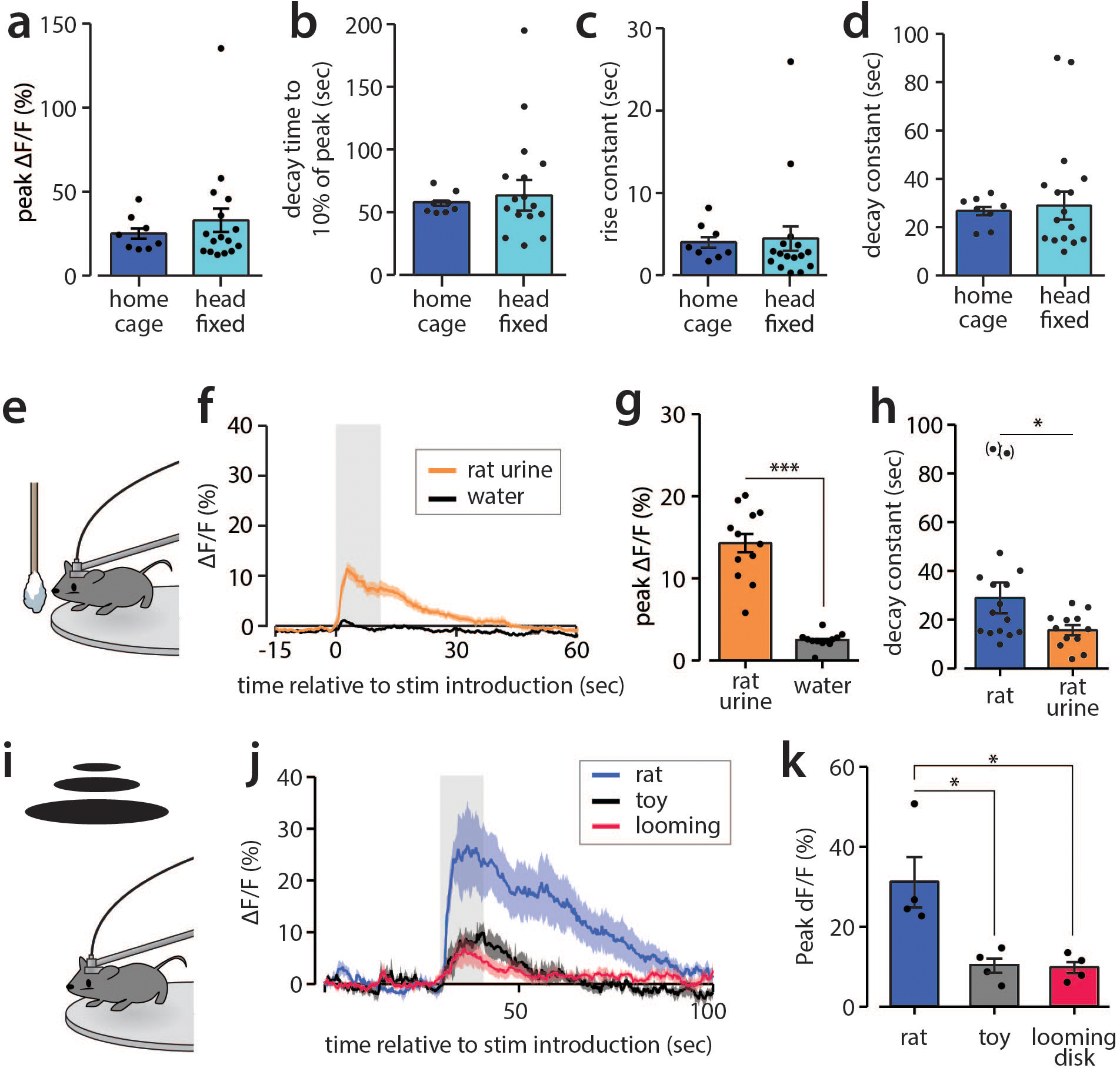
Extended Data 1.
Additional properties of SF1+ neuronsu2019 responses to rat, rat urine, and looming disk stimuli.
a , Peak u0394F/F activity in response to rat in homencage (anaesthetized, uncaged stimulus) and a head-fixed set-up (awake, cagednstimulus). (home cage group n = 4 mice; head-fixed group n = 6 mice; ...
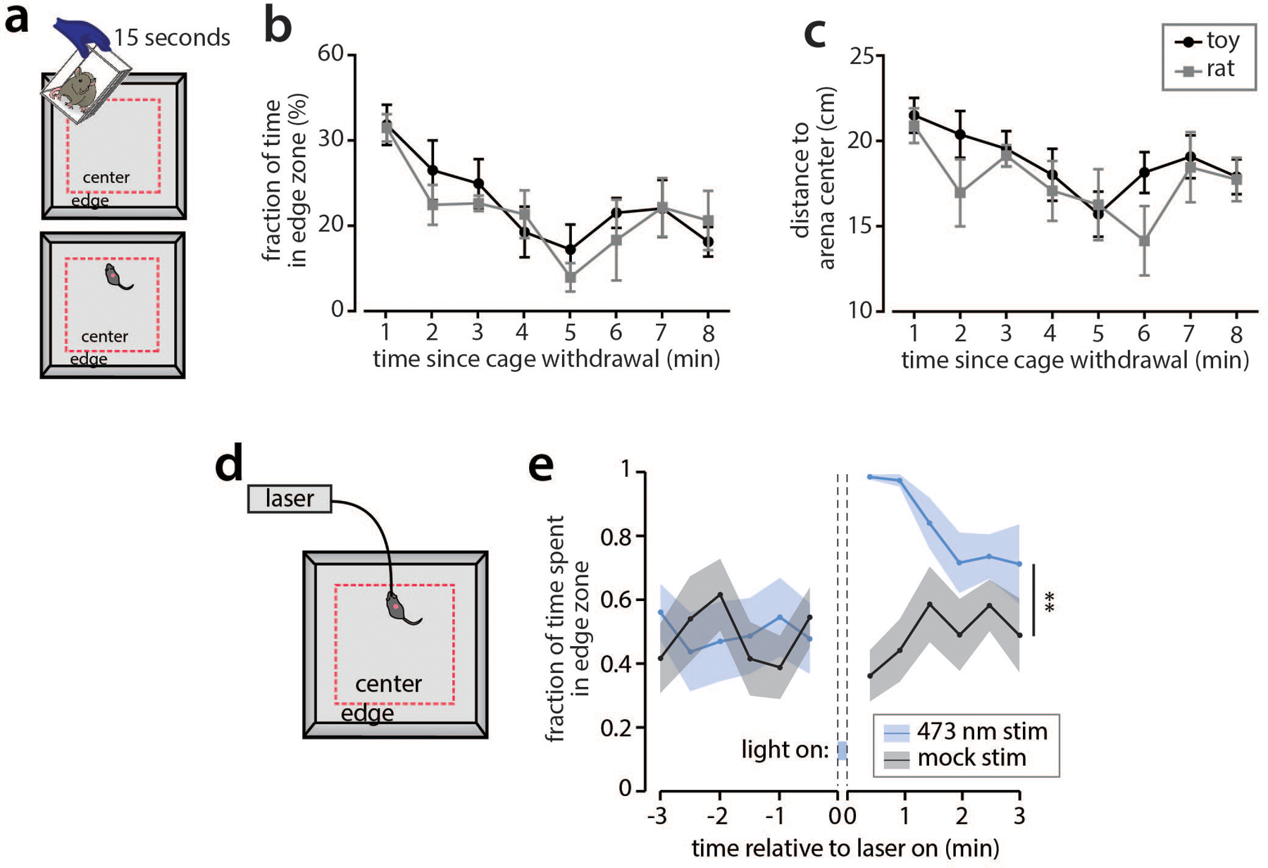
Extended Data 2.
No change in mouse behavior due to potential lingering odor from rat.
a , Schematic plot showing experiment protocol: top, anlive rat or toy rat (control) was brought to the open field arena in a wirenmesh cage for 15 seconds; bottom, mouse was introduced to arena after...
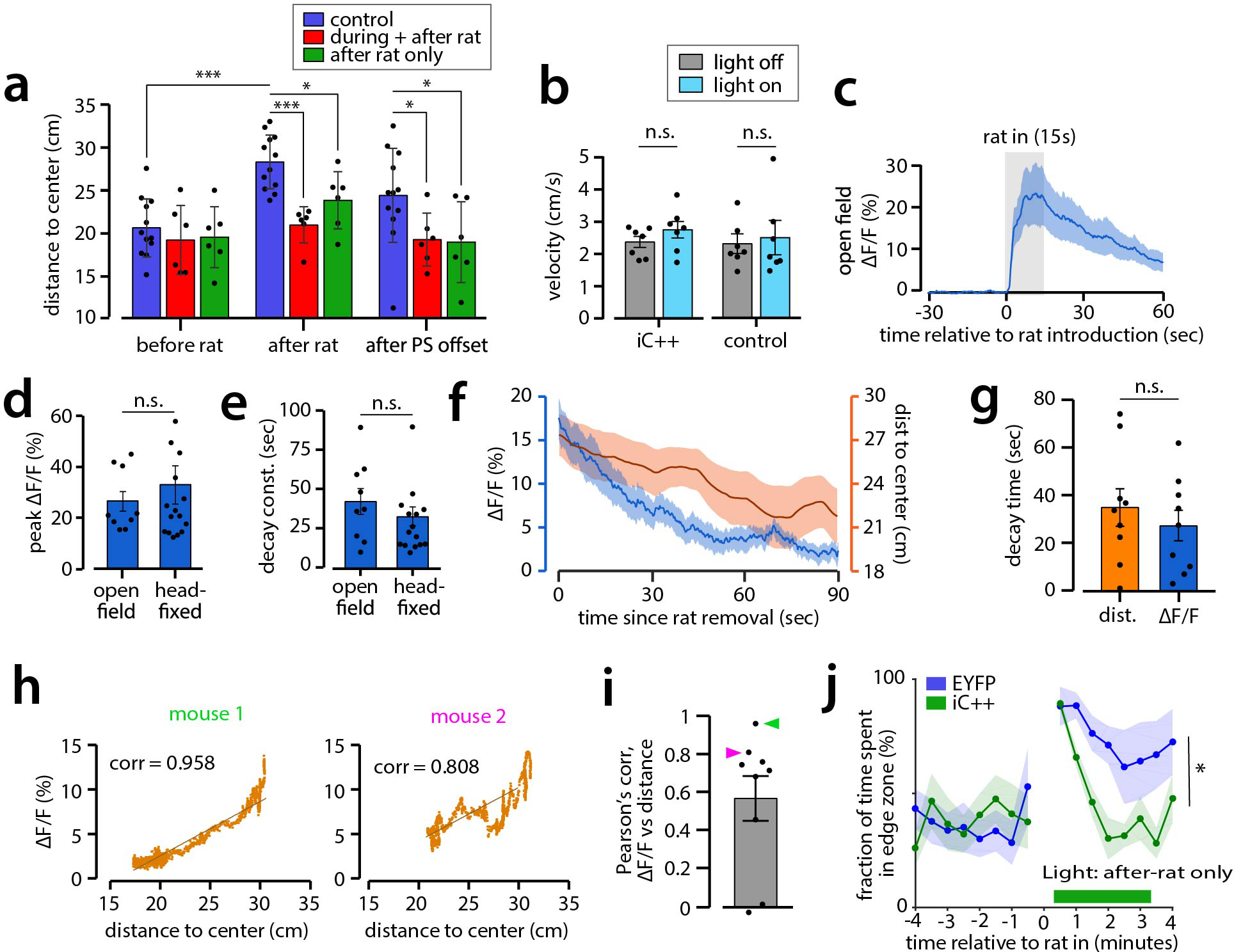
Extended Data 3.
Fiber photometry and VMHdm SF1 neuron silencing in open field rat exposure assay.
a , Distance from mouse body center to arena centernduring three different time periods: before rat, after rat and afternphotostimulation offset, corresponding to u20131 u2013 0, 0 u2013 1nand 3 u2013...
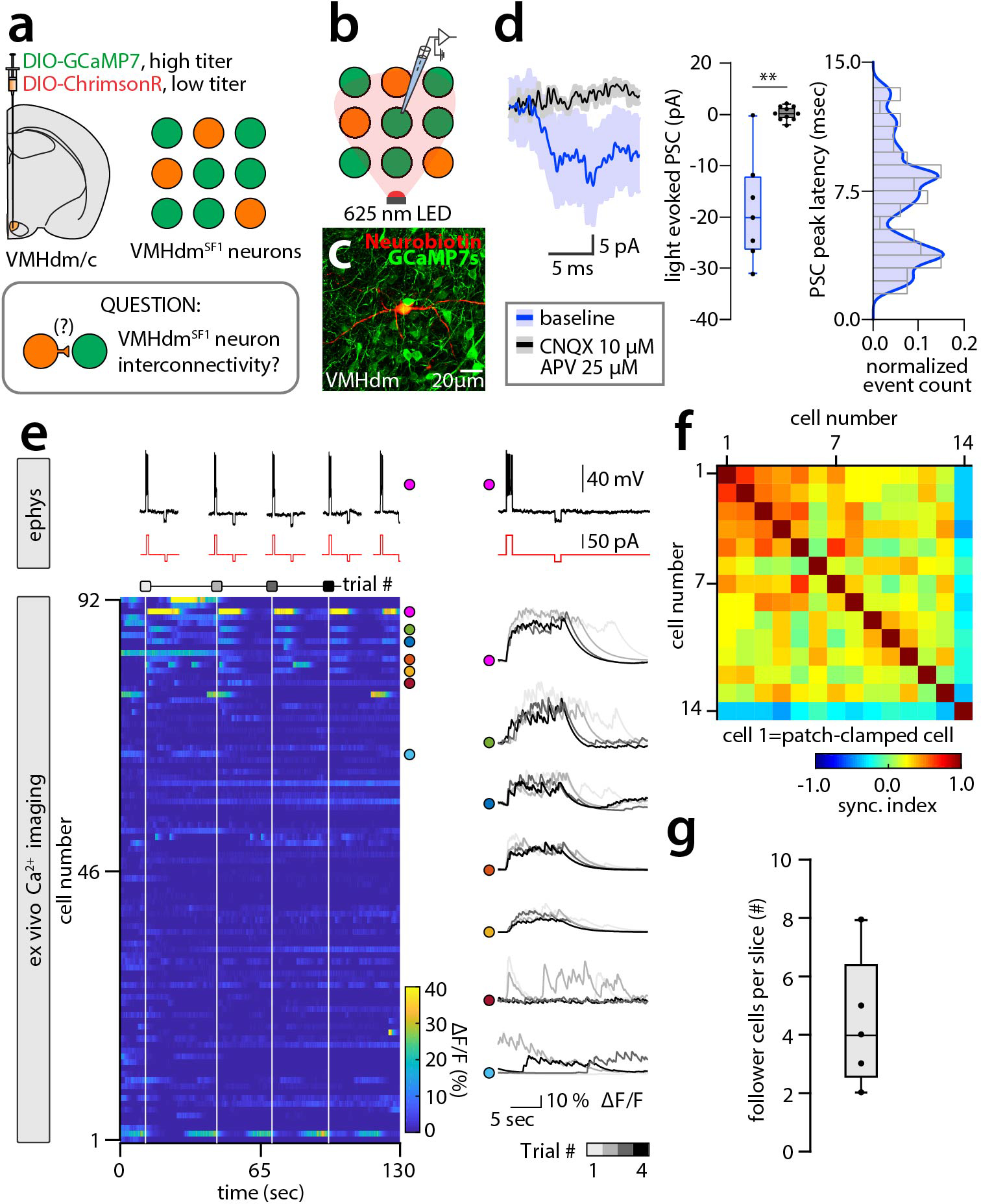
Extended Data 4.
Excitatory monosynaptic interconnectivity in VMHdm SF1 neurons, sensitive to glutamate receptor blockade.
a , Schematic illustration of the experimental designnused to transduce the majority of VMHdmSF1 neurons with Cre-dependentnGCaMP7s and a minority of VMHdmSF1 neurons with Cre-dependentnChrimsonR-tdTo...
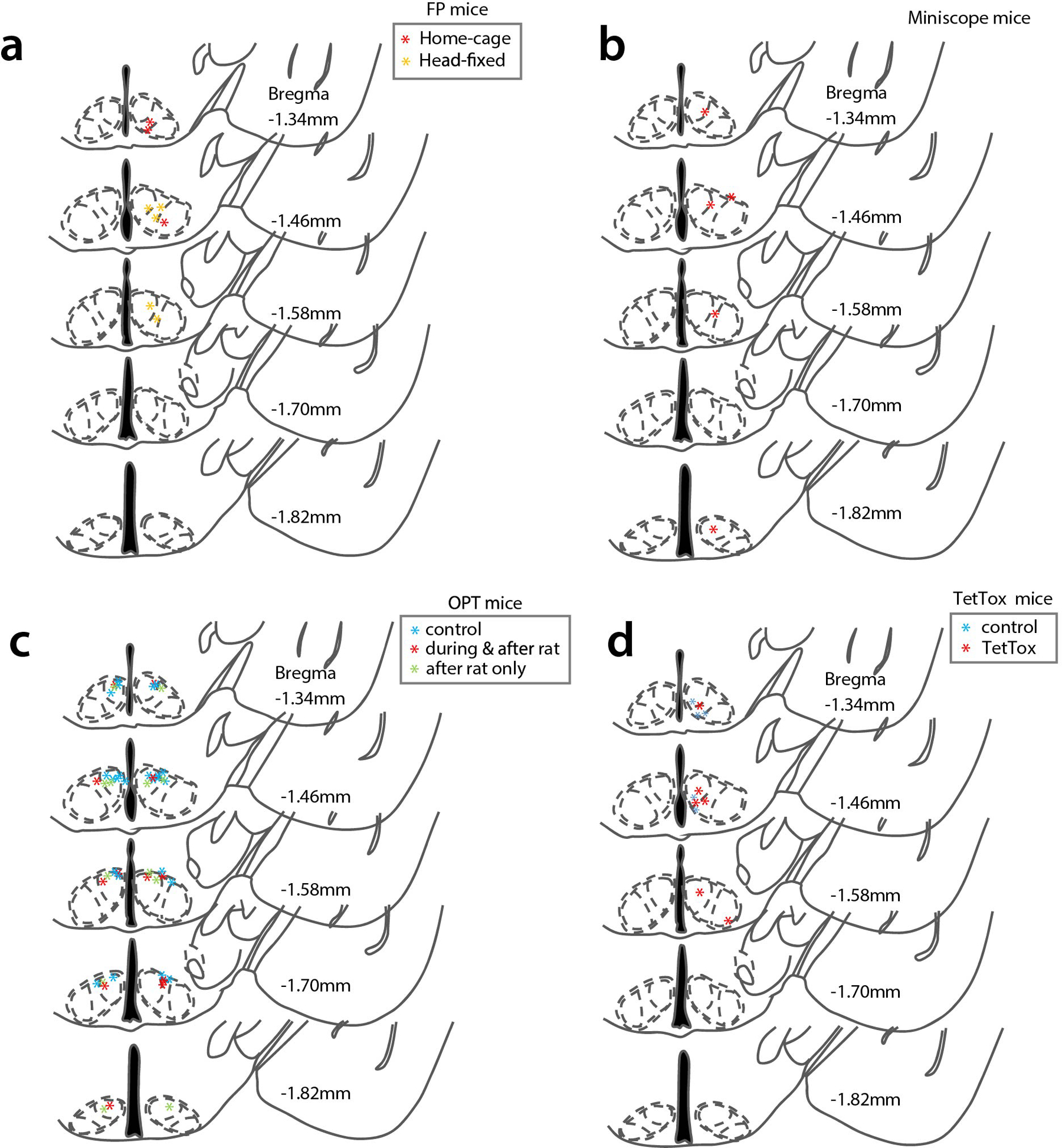
Extended Data 5.
Summary of fiber/GRIN lens placements.
a, Map of the recording sites for fiber-photometry micenincluded in Figure 1 . b, Map of the microscope GRIN lens location for mice illustrated in Figures 2 u2013 3 . c, Map of the fiber tip locations...
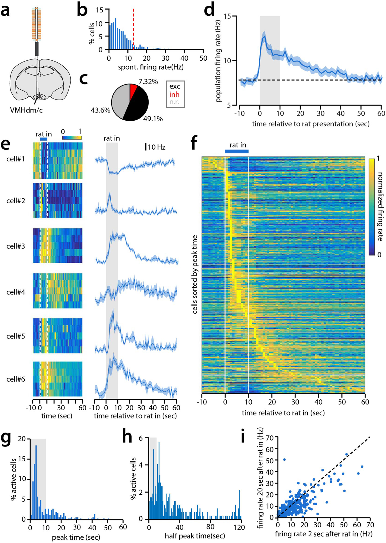
Extended Data 6.
Confirmation of VMHdm/c population dynamics using in-vivo electrophysiology.
a , Schematic illustrating silicon probe recording fromnVMHdm/c in head-fixed mouse. b , Histogram of the spontaneousnfiring rate of all recorded cells in VMHdm. Red dotted line indicates thatn90% of ...
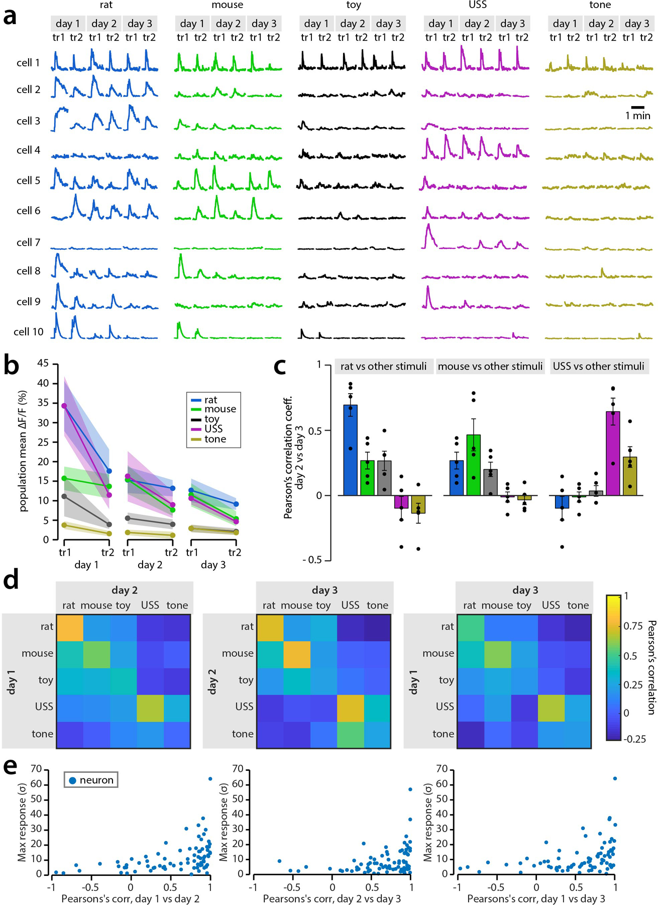
Extended Data 7.
Stability of the VMHdm SF1 population response across trials and days.
a , Responses of ten example VMHdm SF1 neuronsnacross three days of imaging, from the n=5 microendoscopic imaging mice. Thenfive stimuli are presented for two trials (tr1, tr2) each day innpseudorando...
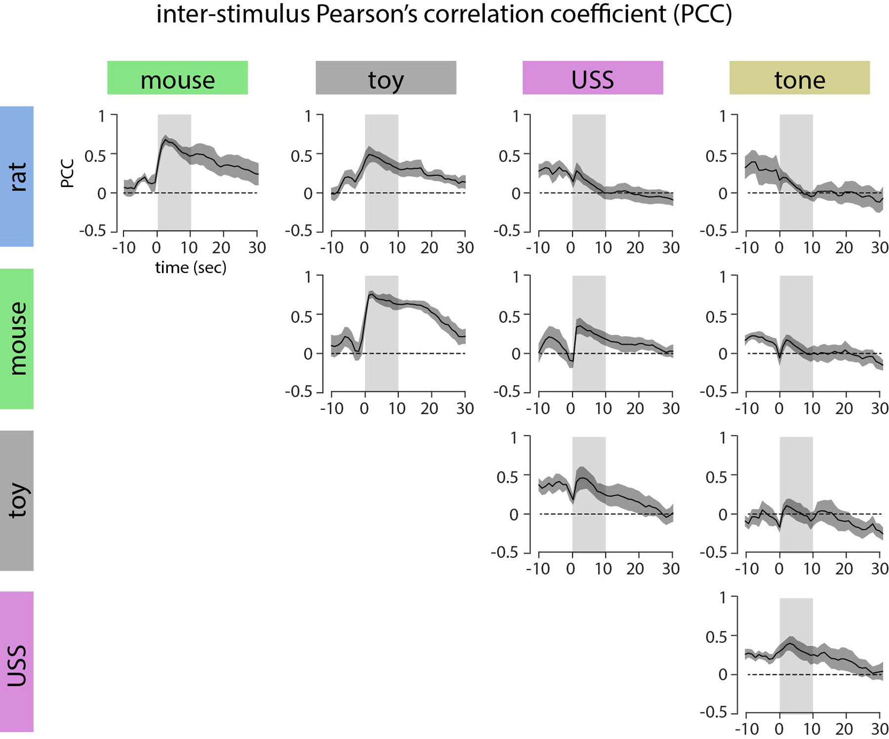
Extended Data 8.
Additional Pearsonu2019s correlations between stimulus pairs.
Pearsonu2019s correlation between VMHdm SF1 populationnactivity as a function of time, evoked by all possible pairs of stimuli (n=5nimaged mice; mean u00b1 SEM).
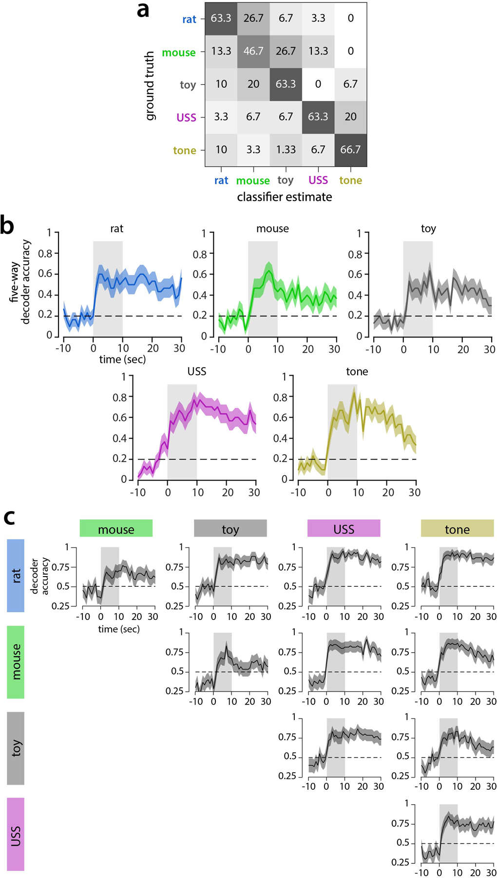
Extended Data 9.
Additional decoder analysis of VMHdm SF1 population activity.
a, Confusion matrix of the five-way Nau00efve Bayesndecoder shown in Figure 3n , showingnpredicted stimulus identity for each stimulus class. Matrix is normalized sonrows sum to 100%. b, Accuracy of a...
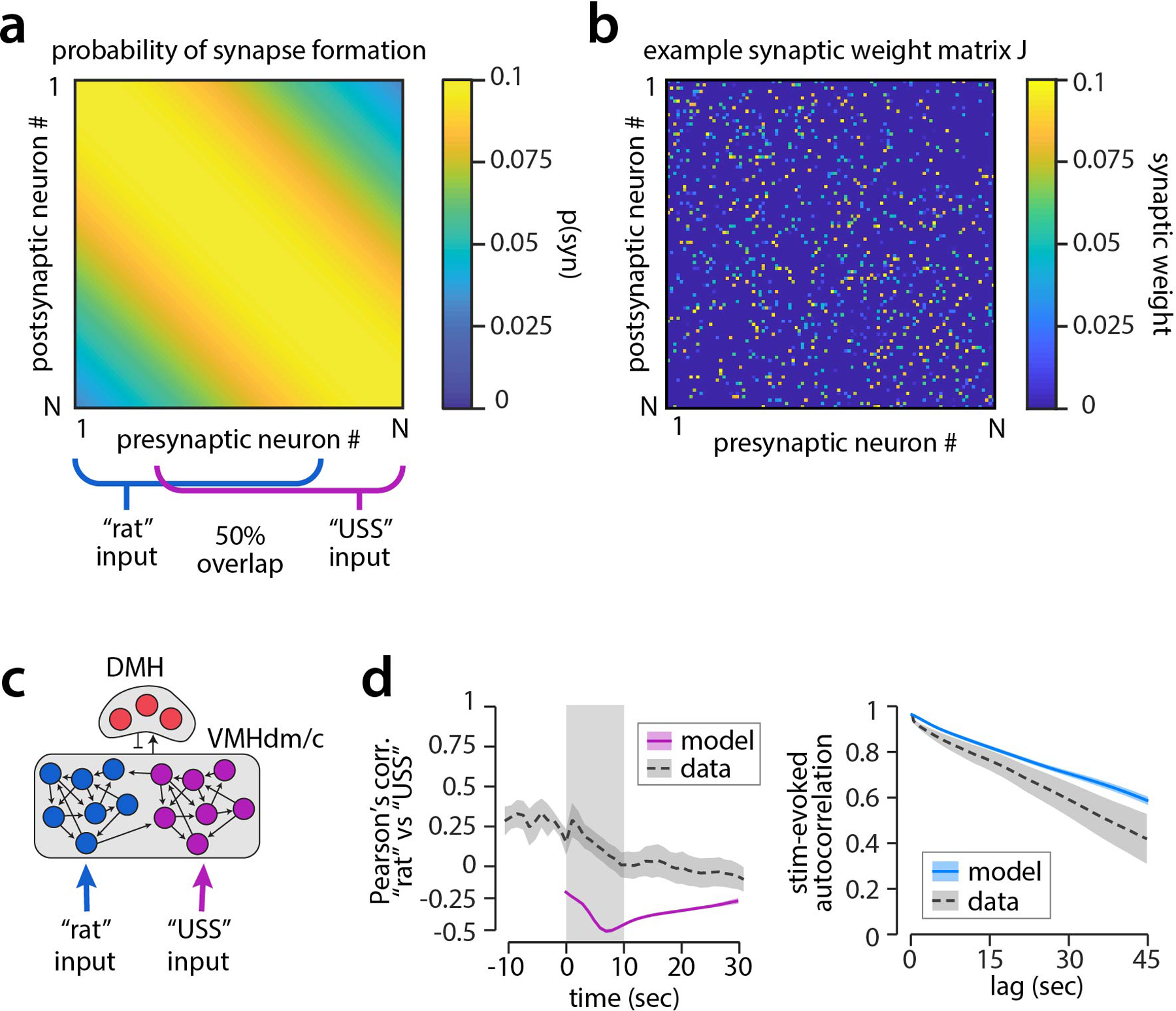
Extended Data 10.
Locally connected model networks.
a, Probability of synapse formation between neuronnpairs decreases moderately as a function of u201cdistanceu201d (neuronnnumber) in the locally connected sRNN model. Segments of the model targetednby...
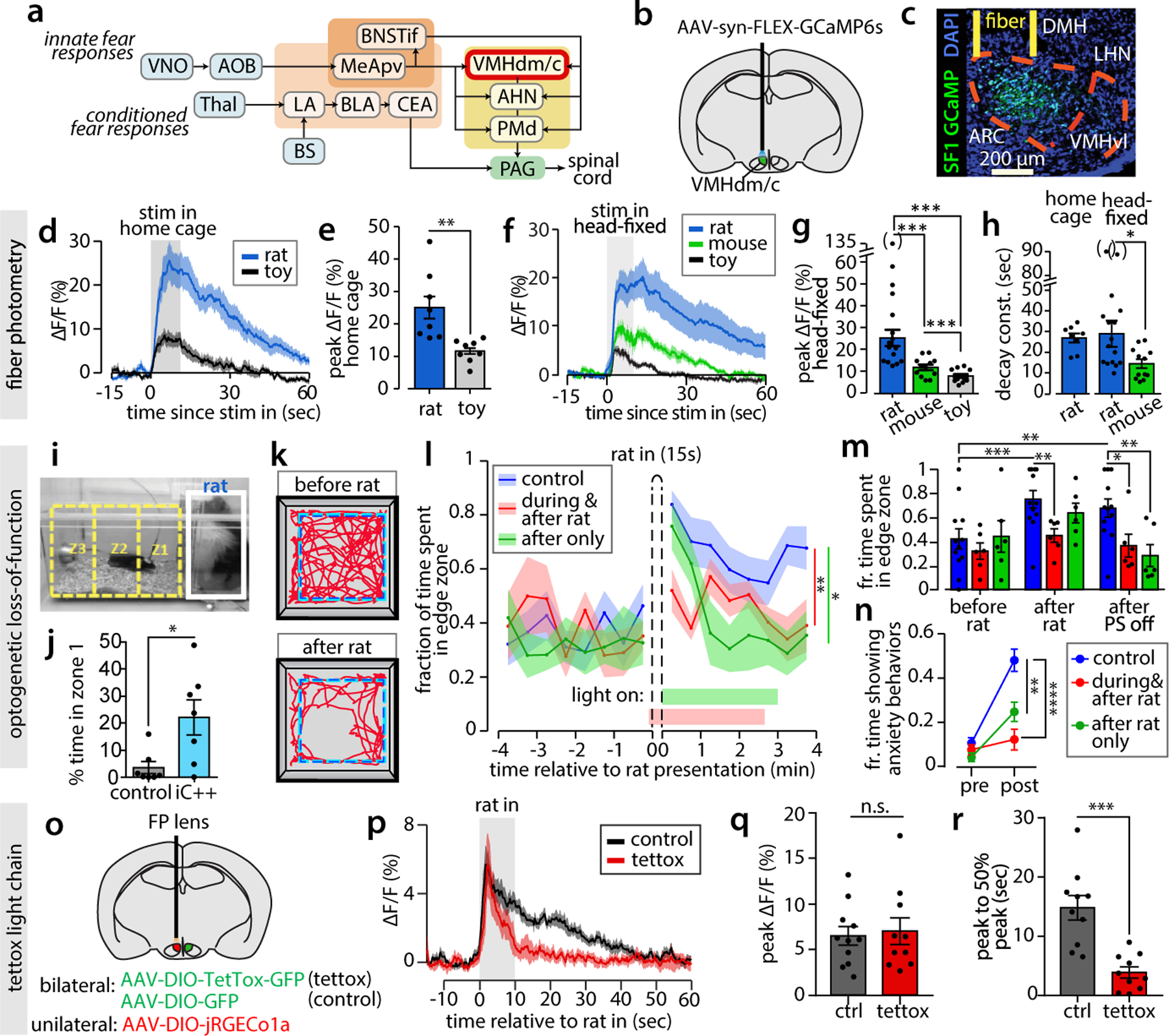
Figure 1.
Persistent activity in VMHdm SF1 neurons evoked by predatory and conspecific cues.
For all plots in all figures, ns = p>=0.05, * = p<0.05, **n= p<0.01, *** = p<0.001, **** = 0<0.0001. Exact p-valuesnand statistical tests used are reported in Supplementary Table 1 . a , C...
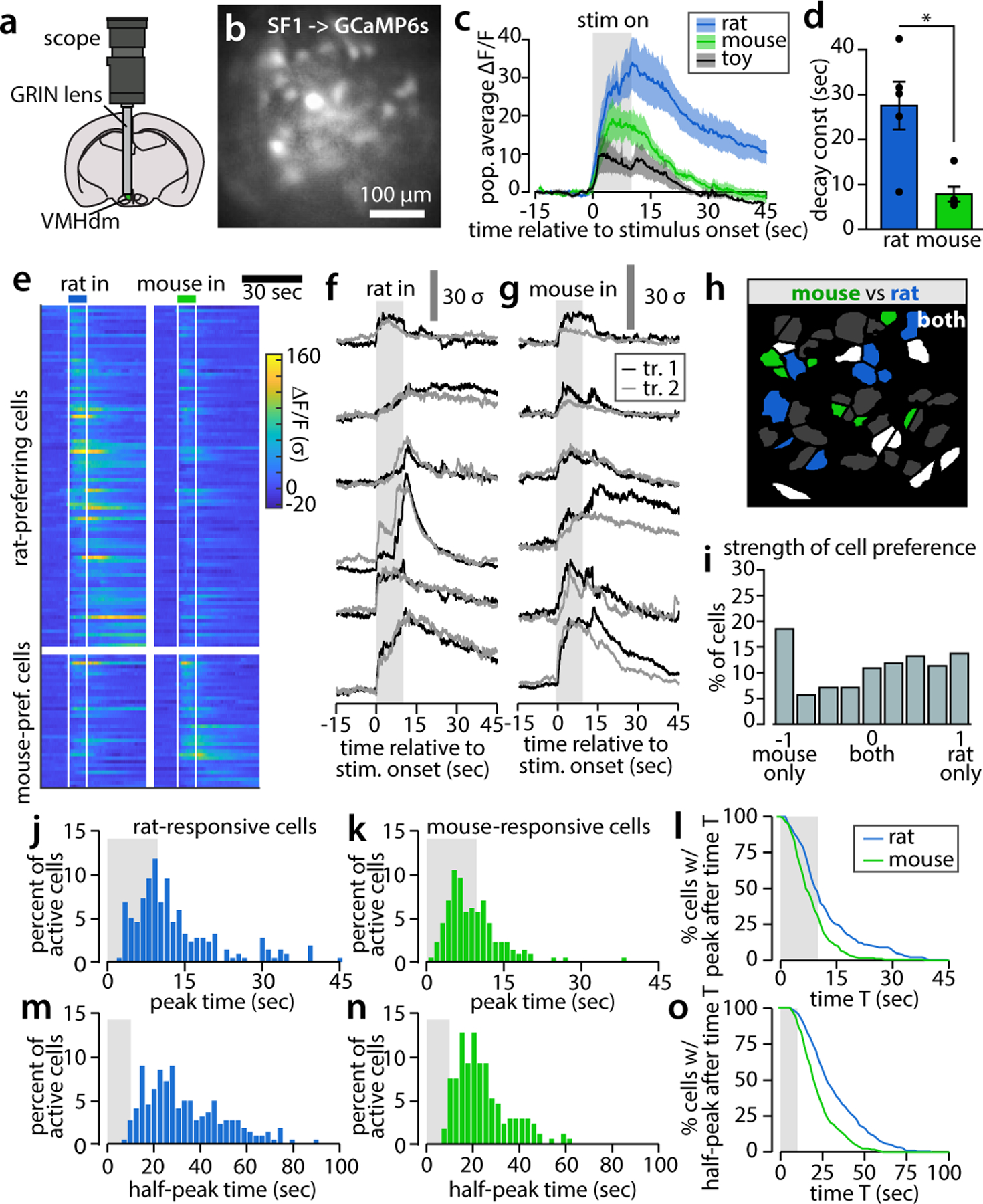
Figure 2.
Microendoscopic imaging reveals persistence emerges from population activity.
a , Microendoscopic imaging in VMHdm/c. b ,nField of view in an imaged mouse. c , Mean population response ofnimaged neurons to each stimulus (n = 2 trials/mouse from 5 mice, mean u00b1nSEM). d , Fit ...
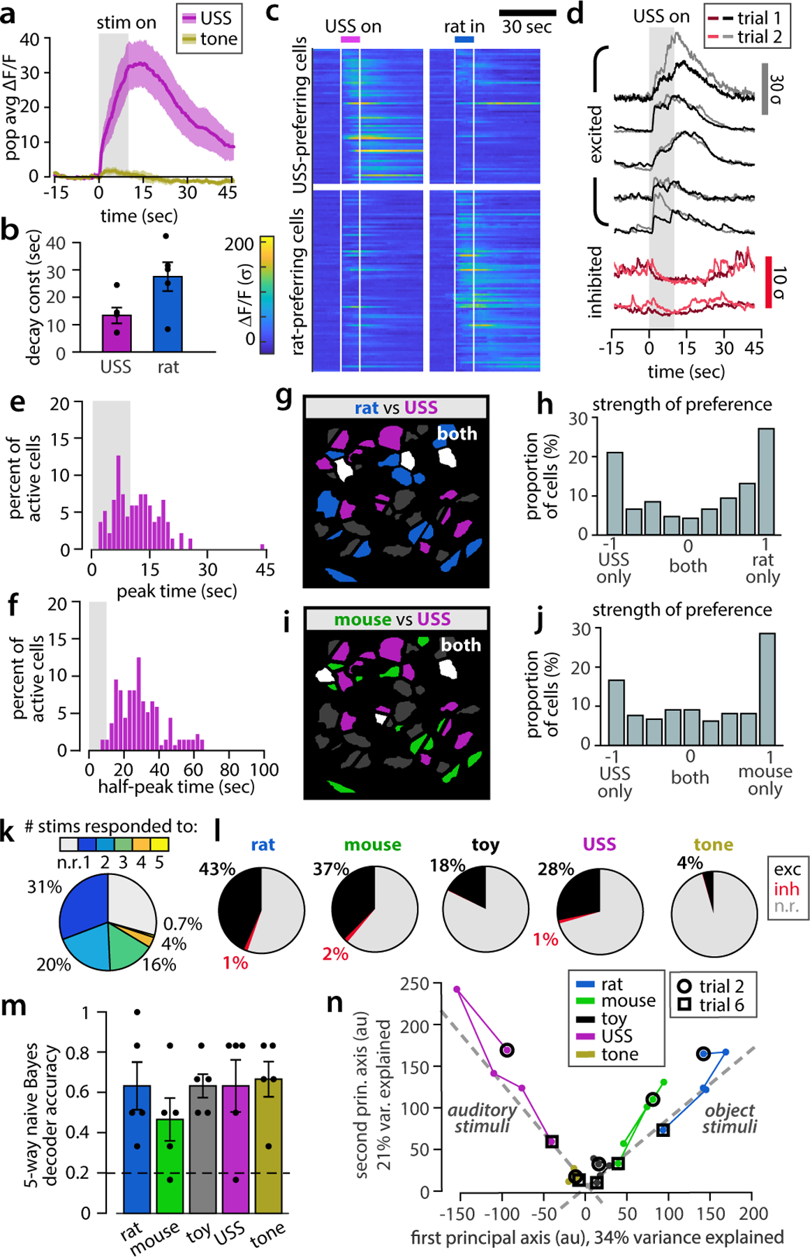
Figure 3.
VMHdm SF1 neurons respond to a threatening auditory stimulus, and encode stimulus identity.
a , Mean VMHdm SF1 population response to aversivenUSS and 2 kHz tone (n = 5 mice, mean u00b1 SEM). b, Fit decaynconstants of population response to USS (rat reproduced from Fig 2d for comparison, mea...
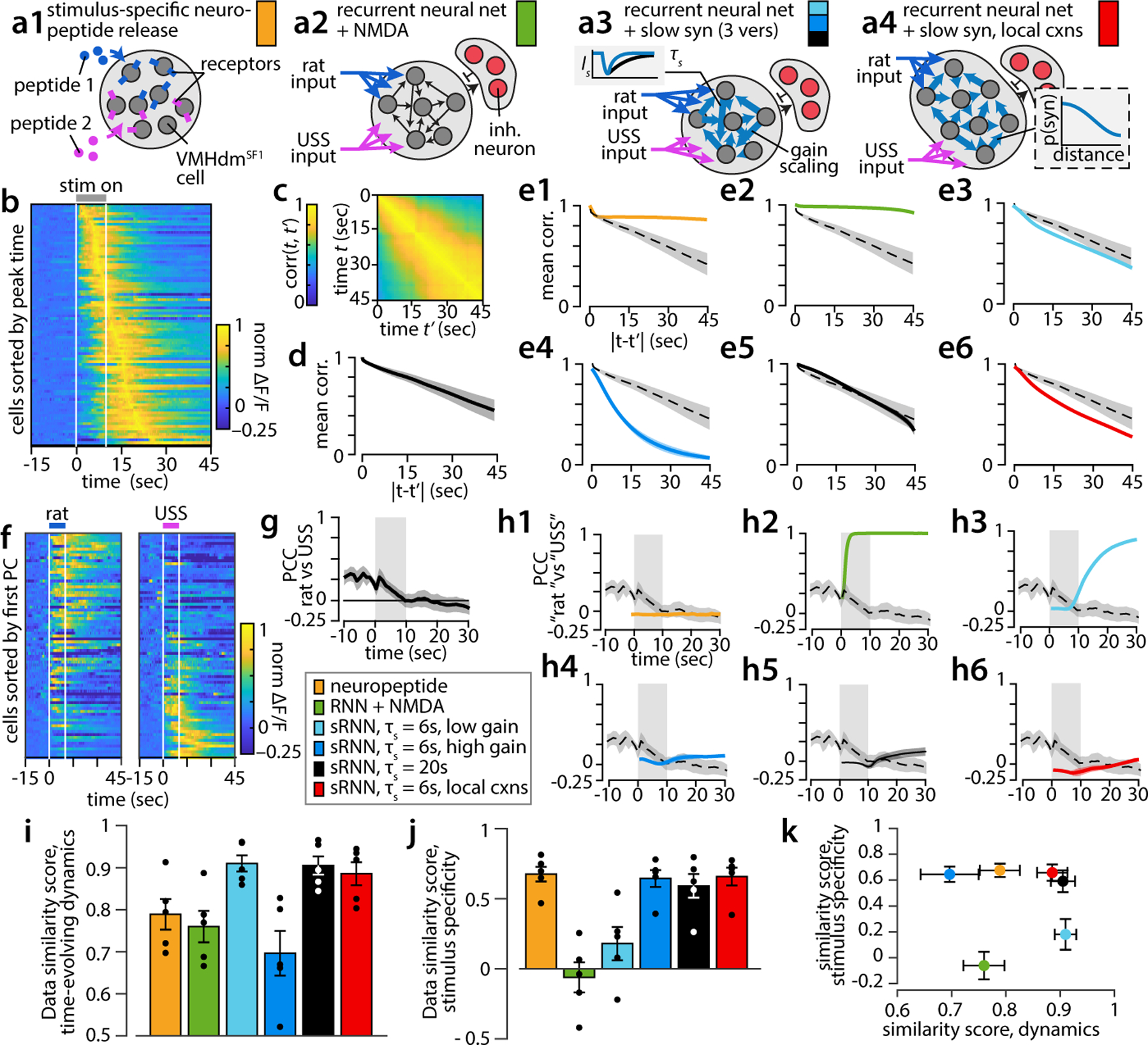
Figure 4.
Data constrain set of computational models for persistent neural activity.
a , Six tested models of persistent activity. a1 , slow-acting neuropeptide (or other neuromodulator)nactivation, no local connectivity between model neurons. a2 ,nrecurrent excitation in a randomly c...
Figure images are served from the NIH/NLM PubMed Central Open Access Subset or Europe PMC; copyright remains with the publishers and authors.
💬 Discussion
0 commentsNo comments yet. Be the first to start a discussion!
Leave a Comment