Abstract
Super-resolution structured illumination microscopy (SIM) has become a widely used method for biological imaging. Standard reconstruction algorithms, however, are prone to generate noise-specific artifacts that limit their applicability for lower signal-to-noise data. Here we present a physically realistic noise model that explains the structured noise artifact, which we then use to motivate new complementary reconstruction approaches. True-Wiener-filtered SIM optimizes contrast given the available signal-to-noise ratio, and flat-noise SIM fully overcomes the structured noise artifact while maintaining resolving power. Both methods eliminate ad hoc user-adjustable reconstruction parameters in favor of physical parameters, enhancing objectivity. The new reconstructions point to a trade-off between contrast and a natural noise appearance. This trade-off can be partly overcome by further notch filtering but at the expense of a decrease in signal-to-noise ratio. The benefits of the proposed approaches are demonstrated on focal adhesion and tubulin samples in two and three dimensions, and on nanofabricated fluorescent test patterns.
🔬 Techniques
🔭 Microscopes
✨ Fluorophores
🧪 Sample Preparation
🔬 Cell Lines
🏭 Microscope Brands
🧪 Reagent Suppliers
📷 Detectors
💻 Software Details
💾 Data Repositories
🏛️ Research Organizations (ROR)
Affiliated research institutions:
📋 Methods
Microscope setups Images for Figure 1 , 2 , 3 , and 5 and Extended Data Figure 1 , 2 , 4 , and 5 are acquired with a commercial Zeiss Elyra PS1 system, using a 63×/1.40 oil immersion objective and a 1004×1002, 8 μm pixel, Andor iXon3 885 EM-CCD camera. A magnification adapted tube lens is used giving rise to a 79 nm back-projected pixel size. Raw images are acquired for five rotations and five translations of the line illumination pattern. Images for Figure 4 and Extended Data Figure 6 , 7 , 8 , 9 , and 10 are acquired with a commercial DeltaVision OMX V3 Blaze (GE Healthcare) instrument, using a 60x/1.42 PlanApo oil immersion objective (Olympus) and a 2048×2048, 6.5 μm pixel, PCO edge 4.2 sCMOS cameras with a magnification adapted tube lens giving rise to a 82 nm back-projected pixel size. Raw images are acquired for three rotations and five translations of the line illumination pattern. The raw images used for the reconstructions shown in Extended Data Figure 3 are recorded with a DMD-SIM setup described in detail elsewhere 26 . In short, multi-spot arrays with a pitch of 10 DMD-pixels (DMD pixelsize 13.68 μm) were created using 488 nm despeckled laser illumination and projected onto the sample via a relay path and a 60×/0.7 air objective (projected DMD-pixel size 137 nm) of an Olympus IX71 microscope and subsequently scanned across the sample. The images were captured on a 2048×2048, 6.5 μm pixel, Hamamatsu Orca Flash 4.0 camera (projected pixel size 108 nm). Samples Figure 1 , 2 and 5 , Extended Data Figure 1 , and Supplementary Figure 5 show data of GFP-zyxin expressing U2OS cells. Zyxin is an integral protein in focal adhesions, protein complexes that form a connection between the extracellular matrix through integrin receptors and the actin cytoskeleton, through its interaction with α-actinin 40 and the stretch sensitive protein p130 cas in which it acts as one of the mechanosensing components in focal adhesions 41 , 42 . Sterile high precision coverslips #1.5H (Marienfeld Superior) were incubated with 10 μg/ml purecol (Advanced Biomatrix) overnight at 4°C and subsequently washed three times with PBS. U2OS cells were grown in DMEM and transfected with GFP-zyxin (a kind gift from Johan de Rooij). The cells were fixed for 20 min in 4% formaldehyde/PBS and mounted on a glass slide in Vectashield antifade mounting medium (Vectorlabs). Cells grown on collagen coated coverslips typically show rod shaped focal adhesions, consisting of parallel linear structures 23 , additionally zyxin is observed to be present on actin fibers in distinct patches. Figure 3 and Extended Data Figure 4 show data of nano-fabricated fluorescent test structures patterned using a previously published method 43 , that was slightly adopted for higher resolution patterning. In short, a monolayer of 3-[Methoxy(polyethyleneoxy)propyl]trimethoxysilane (ABCR, Germany) was covalently grafted onto ITO-coated no.1 cover glass (Optics Balzers) and locally exposed to a focused electron beam following the defined patterns. After removal from the SEM, the sample was incubated for 45 minutes with a 100nM IgG-Alexa Fluor 488 solution in 1X TE buffer. Samples were then washed with TE buffer and deionized water, followed by drying and transfer to the optical microscope. Extended Data Figure 5 show data of the mCherry-SYCP3 protein in the synaptonemal complex. Mouse oocytes from mice expressing mCherry-SYCP3 44 were isolated and spread 45 on #1.5H high precision coverslips and embedded in prolong gold (Invitrogen). SYCP3 is part of the lateral element of the synaptonemal complex (SC) that is formed during meiosis prophase I. The synaptonemal complex is comprised of two lateral elements that form parallel linear protein assemblies at a distance of ~220 nm apart 46 . Figure 4 , Extended Data Figure 6 , and Supplementary Movies 3 to 6 show data of collected of 4% formaldehyde fixed mouse C127 cells grown on #1.5H high precision coverslips, immunostained for microtubules using DM1A mouse monoclonal anti-α-Tubulin primary antibodies (Sigma-Aldrich) and donkey anti-mouse Alexa Fluor 488 secondary antibodies (ThermoFisher), and mounted in Vectashield H-1000 medium (Vector Labs). Extended Data Figure 7 shows data of a monolayer of 100 nm yellow-green Fluosphere beads (ThermoFisher), dried and mounted in glycerol 18 . Extended Data Figure 9 and Supplementary Movie 8 show data of a 2% formaldehyde fixed C127 cell immune-labelled with rabbit anti-histone H3K4me3 primary antibodies (Active Motif) and goat-anti rabbit Alexa Fluor 488 secondary antibodies (ThermoFisher), counterstained with DAPI and mounted in Vectashield. Supplementary Movie 9 and Extended Data Figure 10 show live cell data of stably expressing histone H2B-GFP grown in a 35 mm μ Dish with high precision glass bottom (Ibidi) and imaged at 37° and 5% CO 2 . A time series was recorded with 2s intervals. For each time point 7 z-sections with z-distance of 0.125 μm were acquired (in total 7x3x5=105 raw images per time point). Extended Data Figure 2 , 3 , 8 and Supplementary Movie 7 show data of a bovine pulmonary artery endothelial cell (BPAEC), with mitochondria labelled with MitoTracker Red, actin labeled with Alexa Fluor 488, and DNA labeled with DAPI, and embedded in hardening mounting medium (Thermo Fisher Fluo Cells slide #1).
Show full methods section
Microscope setups Images for Figure 1 , 2 , 3 , and 5 and Extended Data Figure 1 , 2 , 4 , and 5 are acquired with a commercial Zeiss Elyra PS1 system, using a 63×/1.40 oil immersion objective and a 1004×1002, 8 μm pixel, Andor iXon3 885 EM-CCD camera. A magnification adapted tube lens is used giving rise to a 79 nm back-projected pixel size. Raw images are acquired for five rotations and five translations of the line illumination pattern. Images for Figure 4 and Extended Data Figure 6 , 7 , 8 , 9 , and 10 are acquired with a commercial DeltaVision OMX V3 Blaze (GE Healthcare) instrument, using a 60x/1.42 PlanApo oil immersion objective (Olympus) and a 2048×2048, 6.5 μm pixel, PCO edge 4.2 sCMOS cameras with a magnification adapted tube lens giving rise to a 82 nm back-projected pixel size. Raw images are acquired for three rotations and five translations of the line illumination pattern. The raw images used for the reconstructions shown in Extended Data Figure 3 are recorded with a DMD-SIM setup described in detail elsewhere 26 . In short, multi-spot arrays with a pitch of 10 DMD-pixels (DMD pixelsize 13.68 μm) were created using 488 nm despeckled laser illumination and projected onto the sample via a relay path and a 60×/0.7 air objective (projected DMD-pixel size 137 nm) of an Olympus IX71 microscope and subsequently scanned across the sample. The images were captured on a 2048×2048, 6.5 μm pixel, Hamamatsu Orca Flash 4.0 camera (projected pixel size 108 nm). Samples Figure 1 , 2 and 5 , Extended Data Figure 1 , and Supplementary Figure 5 show data of GFP-zyxin expressing U2OS cells. Zyxin is an integral protein in focal adhesions, protein complexes that form a connection between the extracellular matrix through integrin receptors and the actin cytoskeleton, through its interaction with α-actinin 40 and the stretch sensitive protein p130 cas in which it acts as one of the mechanosensing components in focal adhesions 41 , 42 . Sterile high precision coverslips #1.5H (Marienfeld Superior) were incubated with 10 μg/ml purecol (Advanced Biomatrix) overnight at 4°C and subsequently washed three times with PBS. U2OS cells were grown in DMEM and transfected with GFP-zyxin (a kind gift from Johan de Rooij). The cells were fixed for 20 min in 4% formaldehyde/PBS and mounted on a glass slide in Vectashield antifade mounting medium (Vectorlabs). Cells grown on collagen coated coverslips typically show rod shaped focal adhesions, consisting of parallel linear structures 23 , additionally zyxin is observed to be present on actin fibers in distinct patches. Figure 3 and Extended Data Figure 4 show data of nano-fabricated fluorescent test structures patterned using a previously published method 43 , that was slightly adopted for higher resolution patterning. In short, a monolayer of 3-[Methoxy(polyethyleneoxy)propyl]trimethoxysilane (ABCR, Germany) was covalently grafted onto ITO-coated no.1 cover glass (Optics Balzers) and locally exposed to a focused electron beam following the defined patterns. After removal from the SEM, the sample was incubated for 45 minutes with a 100nM IgG-Alexa Fluor 488 solution in 1X TE buffer. Samples were then washed with TE buffer and deionized water, followed by drying and transfer to the optical microscope. Extended Data Figure 5 show data of the mCherry-SYCP3 protein in the synaptonemal complex. Mouse oocytes from mice expressing mCherry-SYCP3 44 were isolated and spread 45 on #1.5H high precision coverslips and embedded in prolong gold (Invitrogen). SYCP3 is part of the lateral element of the synaptonemal complex (SC) that is formed during meiosis prophase I. The synaptonemal complex is comprised of two lateral elements that form parallel linear protein assemblies at a distance of ~220 nm apart 46 . Figure 4 , Extended Data Figure 6 , and Supplementary Movies 3 to 6 show data of collected of 4% formaldehyde fixed mouse C127 cells grown on #1.5H high precision coverslips, immunostained for microtubules using DM1A mouse monoclonal anti-α-Tubulin primary antibodies (Sigma-Aldrich) and donkey anti-mouse Alexa Fluor 488 secondary antibodies (ThermoFisher), and mounted in Vectashield H-1000 medium (Vector Labs). Extended Data Figure 7 shows data of a monolayer of 100 nm yellow-green Fluosphere beads (ThermoFisher), dried and mounted in glycerol 18 . Extended Data Figure 9 and Supplementary Movie 8 show data of a 2% formaldehyde fixed C127 cell immune-labelled with rabbit anti-histone H3K4me3 primary antibodies (Active Motif) and goat-anti rabbit Alexa Fluor 488 secondary antibodies (ThermoFisher), counterstained with DAPI and mounted in Vectashield. Supplementary Movie 9 and Extended Data Figure 10 show live cell data of stably expressing histone H2B-GFP grown in a 35 mm μ Dish with high precision glass bottom (Ibidi) and imaged at 37° and 5% CO 2 . A time series was recorded with 2s intervals. For each time point 7 z-sections with z-distance of 0.125 μm were acquired (in total 7x3x5=105 raw images per time point). Extended Data Figure 2 , 3 , 8 and Supplementary Movie 7 show data of a bovine pulmonary artery endothelial cell (BPAEC), with mitochondria labelled with MitoTracker Red, actin labeled with Alexa Fluor 488, and DNA labeled with DAPI, and embedded in hardening mounting medium (Thermo Fisher Fluo Cells slide #1).
SIM processing and reconstruction
The data shown in Figure 1 , 2 , 3 , and 5 and Extended Data Figure 1 , 2 , 4 and 5 pertain to 2D-SIM reconstructions made from a single focal slice of a 3D-SIM acquisition, i.e. made with a three-beam interference illumination pattern. The data shown in Figure 4 and Extended Data Figure 6 , 7 , 8 , 9 and 10 pertain to full 3D-SIM reconstructions. A flow diagram illustrating the different steps in making (2D and 3D) SIM reconstructions is shown in Supplementary Figure 6 , and consists of pre-processing steps, illumination pattern estimation and image Fourier order computation steps, and filtering and reconstruction operations. Pre-processing steps The set of pre-processing operations starts with a gain and offset calibration for providing image signals that represent the number of detected photo-electrons 47 . The EM-CCD or sCMOS cameras that are used have zero or negligible readout noise so that the image signals follow Poisson statistics to a good approximation. Some effects of fixed pattern noise (pixel-to-pixel variations in offset and gain) are visible in sCMOS based images, but are ignored here for the sake of simplicity. In a future study this could possibly be incorporated by an additional camera calibration step, or by extending the method of ref. 47. Optionally, the images are grouped in sets of five images acquired with the same illumination pattern angle, and registered in an all-to-one manner in order to correct for drift. It turns out that leaving out the step of drift correction does not substantially deteriorate the reconstruction outcomes for the imaged specimens. The illumination pattern modulation in 3D-SIM can be characterized by the Modulation Contrast to Noise Ratio (MCNR), a quality measure for faithful illumination pattern retrieval, part of the SIMcheck quality control software package 17 . The proposed method of computation of the MCNR in ref. 17 involves images acquired at different focal planes, and can therefore not be directly applied to 2D-SIM. To that end we use an alternative way to compute the MCNR that can be computed per pixel/voxel. Starting point is a 1D Fourier Transform (FT) of the five phase step images for each pixel/voxel to the set of photon counts N j of each pixel (voxel) for the phase steps j = 1,2,…, M t , resulting in the fit: (5) N j = A 0 + A 1 cos ( 2 π j M t + φ 1 ) + A 2 cos ( 4 π j M t + φ 2 ) The modulation is taken as twice the root-squared average of the first and second order Fourier coefficients A 1 and A 2 , and the shot noise level is the square root of the zeroth Fourier coefficient A 0 . This leads to: (6) M C N R = 2 A 1 2 + A 2 2 A 0 The results obtained with the current proposal for computing the MCNR agree well with the results obtained with SIMcheck, although small quantitative differences appear. For example, the lack of averaging Fourier coefficients over focal slices gives a more noisy appearance of the MCNR across the Field Of View (FOV) for low signal acquisitions. The rule-of-thumb for reliable pattern parameter estimation is to have sufficient foreground pixels/voxels with MCNR ≥ 3. The MCNR is actually a SIM reconstruction in itself, which generalizes the original SIM proposal 1 by including the second order Fourier coefficients, and shows some degree of optical sectioning (see Supplementary Figure 1 ). The peak MCNR averaged over the pattern orientations per focal slice has a maximum as a function of the focal slice (see Supplementary Figure 7 ). Having a satisfactory MCNR only for a limited range of focus positions may be attributed to not just a limited axial extent of the sample, but also to spherical aberration caused by refractive index mismatch. For typical high-NA immersion microscopes the refractive index of the immersion medium must be controlled at the 10 −3 level for optimum results 18 , and the axial range of images with useful modulation appears to be typically only a few μm. For 2D-SIM processing we take the focal slice with the maximum illumination pattern modulation. So-called z-wrapping artefacts 18 may arise for datasets with a limited number of focal slices, as e.g. many live cell 3D datasets. The periodic boundary conditions of the FT then perturb the first and final few of the slices of the reconstruction. This can be mitigated by preferably ignoring these, or by only representing the final SIM reconstruction by a Maximum Intensity Projection of the reconstruction stack. Another method to mitigate the impact of z-wrapping artefacts is by adding a number of extra, fictitious, focus layers. The reconstructions for the live cell dataset of Supplementary Movie 9 and Extended Data Figure 10 , which is based on just 7 focal slices, are made using 14 extra layers. It is estimated that the required number of extra layers is in the range from 10 to 20. These extra focus layers interpolate linearly between the first and last slice of the focus stack. Further, they are blurred by convolution with a Gaussian kernel to mimic the effect of defocus. The kernel size ranges from one pixel for the layers directly adjacent to the first and last focal slice, to 20 pixels for the layer(s) in the middle of the fictitious additional stack. Finally, artificial shot noise is added for maintaining Poisson statistics. The next step in pre-processing is to apply a window to the data cube in order to enforce continuity in the periodic boundary conditions assumed in subsequent FTs, i.e. for eliminating streaking along the coordinate axes in the FTs. For the voxel indices j = 1,…, N along any of the three coordinate axes we can define a scaled coordinate r j = (2 j − 1 − N )/(2 N ), the windowing is applied to the edges defined by 1/2−| r j |≤ b , where we take b in the range 0.1-0.2 along the lateral directions ( r = x and r = y ) and b = 0 along the axial direction ( r = z ). Over these boundary region voxels, the window function is taken to be τ j = sin(π(1−2| r j |)/(4 b )) 2 , for the inner voxels τ j = 1 is taken. The overall window function is the product of the window functions for the three orthogonal coordinate axes. No windowing is applied in the axial direction because it appears to have limited use there. The first and last focal slice typically show no recognizable structure as all object features are drowned by defocus and spherical aberration induced loss of illumination pattern modulation, which implies that the discontinuity arising from the FT periodic boundary conditions in the axial direction is not that harmful. The additional fictitious layers that interpolate between the first and last focal slice, with features that are gradually blurred away, plays the same role for datasets with limited number of focal slices. An additional factor here is that the axial Fourier streak is suppressed anyway by the low-pass filtering step with the 3D-OTF of the microscope, which has the well-known missing cone. The windowing operation by a simple pointwise multiplication of the image data cube with the window function compromises Poisson statistics of the image signals. This can be overcome by applying the random binomial data splitting approach (see Supplementary Note 2 ). The image signal for a pixel is written as I = n + ε, where n = round ( I ). The value of the window function for this pixel τ satisfies 0≤ τ ≤1 and is used as the probability in a binomial probability distribution for each of the integer n photon counts, giving a random total of n′ counts satisfying 0≤ n ′≤n . The remainder ε is reduced by the ratio n′ / n . This procedure preserves Poisson statistics across the entire data cube. The next pre-processing step is up-sampling in order to accommodate the extended cut-off of the SIM OTF (typically by a factor of 2 in the lateral directions, no up-sampling in the axial direction) by zero padding in Fourier space. This operation compromises Poisson statistics, but this can be solved by artificially filling the extra high spatial frequency Fourier pixels, that are created by zero padding, with noise. For each voxel in the up-sampled image with up-sampled image signal n a random variable n′ is generated using the signal n as Poisson rate. The difference n′ − n , the artificially created noise, is Fourier transformed and masked to fill the new Fourier pixels created by zero padding, while keeping the original Fourier pixels obtained from the FT of n unaltered. Inverse FT then gives an up sampled image that follows Poisson statistics. Illumination pattern parameters and OTF The illumination pattern parameters (pitch, orientation and phases) are estimated using a 2D-projection of the pre-processed 3D dataset. This projection is the (weighted) sum over all focal slices, where the average MCNR values over each focal slice is taken as weight. This improves SNR by averaging over noise in the individual images and over the 3D-structure of the fluorescent object, but under the assumption that these gains are bigger than possible residual shifts in the illumination patterns between different focal slices, left after possible drift correction. Next, the cross-correlation image matrix for all M t × M t image combinations with different pattern phases is computed, zoomed in at regions around integer multiples of the expected Fourier peaks at q → e s t . The peak in the root mean square of the cross-correlation matrix is used to update the estimate of the pattern spatial frequency vector q → e s t (see Supplementary Note 1 for more detail). The precision of peak detection is aided by the zooming capability of the chirp z-transform for evaluating FTs 49 , reaching a relative precision in determining the pitch equal to 6×10 -5 over the K = 10 noise independent acquisitions of the GFP-zyxin dataset and 8×10 -5 over the 15 frames of the live cell histone H2B-GFP dataset. The pattern phases are estimated from the phase of the autocorrelation peaks 50 , reaching a precision of around 1 deg for the GFP-zyxin and for the live cell histone H2B-GFP datasets. The retrieved values for the pitch, orientations, and phases of the illumination patterns are used to compute the different image Fourier orders (0th, 1st, 2nd) per orientation of the line illumination pattern, and to shift these orders in the lateral direction to the correct location in Fourier space. The 3D-OTF is obtained from a bead calibration experiment 18 , if such data is available. The illumination pattern parameters are used to create laterally shifted copies of the different Fourier orders per orientation of the line illumination pattern. An alternative to the calibration OTF is computation using a vectorial Point Spread Function (PSF) model, taking all effects of high NA and polarization into account (see e.g. ref. 48 and references therein). For 3D datasets, this requires an additional axial separation of the two branches of the 1st Fourier order. The theoretical value k z = ±n med (1−cos θ )/ λ ex is used, with λ ex the excitation wavelength, n med the medium refractive index, and sin θ = λ ex / n med p ), where p is the estimated illumination pattern pitch. Finally, the 1st and 2nd order strengths a 1 and a 2 are estimated from the image data itself by requiring consistency across order overlap regions, as the different orders depend on the spatial frequency spectrum of the same underlying fluorescent object (see Supplementary Note 1 for more detail). It turns out that the retrieved order strengths depend on the signal-to-noise ratio and sparsity of the sample, leading to lower estimates for relatively dense samples and/or samples recorded under adverse signal-to-noise conditions. The estimated order strengths should therefore be seen as effective order strengths, not as the true underlying ground truth values. A fixed set of order strengths in the range of values found for the sparse tubulin set of Figure 4 measured at high signal levels ( a 1 = 0.30 and a 2 = 0.45) is used for all SIM reconstructions.
Reconstruction
The functions D ^ j and V ^ j (defined in the Supplementary Note 2 ) are computed from the copies of the incoherent (2D or 3D) OTF, shifted in Fourier space, and from the order strengths a 1 and a 2 . This is sufficient to obtain the regularization filter for flat-noise SIM. For state-of-the-art and true-Wiener SIM we use as apodization filter the trianglex filter  j = Λ ^ j x with Λ ^ j the triangular filter (interpolating linearly between 1 at zero spatial frequency to 0 at the extended SIM cutoff) and x = 0.4 a numerical coefficient, because this has also been used in the literature 13 , 14 . The triangular filter with x = 1 gives a visually similar reconstruction as the Lukosz-bound filter 21 , and is more benign for artefacts, such as the structured noise artefact and the z-wrapping artefact that arises for low number of focal slices, than the trianglex-filter with x = 0.4. An initial pre-Wiener filtered SIM reconstruction is made by low-pass filtering the different image Fourier orders with the corresponding shifted copy of the incoherent OTF, and then adding all contributions weighted with order strengths. Overall Wiener filters A ^ j / ( D ^ j + w ) and 1 / ( D ^ j + w ^ j ) = 1 / V ^ j are applied and a subsequent inverse FT is executed to generate the state-of-the-art and flat-noise SIM reconstructions, respectively. The pre-Wiener filtered SIM reconstruction is used to make an estimate of the Spectral Signal-to-Noise Ratio ( SSNR ) needed for the true-Wiener filtered SIM reconstruction. The initial SIM reconstruction e k rec , i has a spectral power | e ^ j r e c , i | 2 = | e ^ k i + δ e ^ k i | 2 = | e ^ k i | 2 + 2 R e { e ^ k i * δ e ^ k i } + | δ e ^ k i | 2 . Averaging over rings in spatial frequency space effectively eliminates the signal-noise cross-term. The average 〈 N ^ j i 〉 r i n g of the noise power | δ e ^ k i | 2 is independent of the object spectrum and is proportional to the noise variance function V ^ j (see Equation (1b) ). The estimate for the SSNR is then found as: (7) S S N R j ≈ 〈 | e ^ j r e c , i | 2 〉 ring 〈 N ^ j i 〉 ring − 1 which can subsequently be used with Equation (3) to find the regularization filter for the final true-Wiener filtered reconstruction. A minor drawback of ring averaging is that azimuthal variations in SSNR are not accounted for. Averaging schemes based on e.g. Gaussian blurring over regions in spatial frequency space can possibly provide an alternative in case these azimuthal variations become relevant. The error in the estimated SSNR becomes comparable to the SSNR for the highest spatial frequencies, where there is too little signal (see e.g. Figure 1m ). This issue can be solved by extrapolating the regularization filter from low spatial frequencies to high spatial frequencies. The simplest extrapolation is to take the maximum of w ^ ( q → ) for spatial frequencies in the region 〈 S S N R ( q → ) 〉 ring > S S N R thr and use this as a constant regularization in the region 〈 S S N R ( q → ) 〉 ring < S S N R thr . Here, SSNR thr is a threshold value that can typically be selected from the range between about 1 and 10. A bit more complex is a quadratic extrapolation w ^ ( q → ) = α | q → | 2 , where the parameter α is estimated from the spatial frequency region defined by 〈 S S N R ( q → ) 〉 ring > S S N R thr . This corresponds to a regularization function in real space α |▽e| 2 , with ▽ the 2D or 3D-gradient operator 21 . A more general power-law extrapolation w ^ ( q → ) = α | q → | β works fine in many cases as well, where now both parameters α and β are estimated from the spatial frequency region defined by 〈 S S N R ( q → ) 〉 ring > S S N R thr . Typical values found for the power-law exponent β are in the range 1.2 < β < 2.7. For the sake of simplicity we have used the quadratic extrapolation scheme with SSNR thr = 5 for all datasets. Notch filtering of the different image Fourier orders has been applied to improve the optical sectioning in SIM, mostly for 2D-SIM reconstructions 14 , 16 . The retrieved orders (prior to lateral shifting in Fourier space) are multiplied with filter kernels as defined in Equation (3.21), (3.22), and (3.23) in Supplementary Note 3 . The notch depths α 0 , α 1 , α 2 , the lateral notch width △q ‖ , and, for 3D-SIM, the axial notch width △q ⊥ , appearing in the filters are in principle user-adjustable parameters. Instead of an ad-hoc choice, we fix the parameter values to optimize the contrast of flat-noise SIM by making the flat-noise OTF g ^ j F N − S I M = D ^ j / V ^ j as close as possible to a target OTF, which we take to be equal to the Lukosz-bound apodization function. A suitable OTF error function for this optimization is defined in Equation (3.26) in Supplementary Note 3 . Reasonably good results can be obtained for notch widths that scale with the cut-off frequency △ q ‖ = 2 ρ NA / λ ex , and, for 3D-SIM Δ q ⊥ = ρ ( n m e d − n m e d 2 − N A 2 ) / λ e x , where we take the numerical pre-factor ρ = 1.25. For 2D-SIM it is sufficient to apply the notch filtering to the zeroth order only, i.e. α 1 = α 2 =0. The remaining non-zero notch depth α 0 = 1 − 10 −d 0 is determined using Matlab’s fminbnd to find the optimum value of the notch dip exponent d 0 . The procedure converges within about 10 iterations with a precision of around 10 -3 . Typically this results in values in the range 1.5 ≤ d 0 ≤ 3. The final notch filtered images do not depend hugely on the initial choice for the parameter ρ , generally a value ρ > 0.75 will suffice, but small differences can arise between different datasets. The task of optimizing the flat-noise OTF is more complex for 3D-SIM, because the requirement on the axial transfer function comes on top of the requirement on the lateral transfer function, and because the native flat-noise OTF has rather pronounced peaks at the centre spatial frequencies of the contributing orders. It turns out that now applying a notch filter to all contributing orders is necessary, especially as this appears beneficial for diminishing the susceptibility for hexagonal background imprint artefacts. For the sake of simplicity we take α 0 = α 1 = α 2 = 1 − 10 − d n , and again use Matlab’s fminbnd to find the optimum value of the notch dip exponent d n . Typically, this results in values in the range 3.5 ≤ d n ≤ 5.5. It is quite conceivable that more sophisticated designs for the (notch) filters could improve the current results. Noise assessment The noise model is validated by the spectral noise variance and SSNR that are obtained from the K = 10 noise independent acquisitions of the GFP-zyxin dataset by computing the unbiased sample variance over the K reconstructions. The spectral noise variance for the widefield reconstruction obtained by summing over the M r rotations and M t translations appears to be constant across the spatial frequency spectrum with variations up to several percent (see Figure 1i ). The small peak at low spatial frequencies is attributed to residual effects of photo-bleaching, illumination variations, and drift. This small peak gives rise to satellite peaks in the experimental spectral noise variance for the SIM reconstructions at the centre spatial frequencies of the orders, that do not correspond to actual noise enhancement. FRC curves are computed 25 for all K ( K − 1)/2 pairs of reconstructions, the mean and standard deviation over all these reconstruction pairs are plotted in all FRC-results. FRC-curves need no bleaching correction, as they are independent of overall intensity variations of the two input images. The model independent noise assessment via the random binomial data splitting method is described in Supplementary Note 2 . Noise fraction map The noise model enables the assessment of the fraction Z k of the SIM reconstruction that is due to noise, based on the average signal and noise level in a neighbourhood around each pixel k (see Supplementary Note 2 ). We have implemented the computation of this noise fraction by Gaussian smoothing with a width λ /2 NA , which corresponds to about four SIM pixels. For smaller kernel sizes there is insufficient noise averaging, for larger kernel sizes the noise fraction values of the background and of the foreground features is blurred too much. It is expected that 0 ≤ Z k ≤ 1, but values higher than one can arise due to incomplete averaging of noise in the pixel neighbourhood.
Deconvolution and denoising
Starting point for the 2D Richardson-Lucy (RL) deconvolution is a gain recalibration by fitting a straight line through the mean vs. variance curve obtained from the K noise independent reconstructions. This corrects for any possible changes to intensity level during the reconstruction and so ensures the best approximation to Poisson statistics for the signal at each pixel. The reason for this step is that RL-deconvolution can be framed as an object retrieval procedure, based on maximizing a likelihood function that is determined by Poisson statistics 27 . Suitable initial estimates of the non-linear iterative algorithm are either the recorded widefield image (RL-widefield) or the flat-noise SIM reconstruction (RL-SIM). The OTF used in the RL deconvolution algorithm is either the incoherent OTF (RL-widefield) or the flat-noise SIM OTF (RL-SIM). The iterative procedure is stopped when the error ( ∑ k ( e k n + 1 − e k n ) 2 ) / ( ∑ k ( e k n ) 2 ) , with e k n the n -th estimate, is less than 10 −5 . The resulting RL-SIM deconvolution has been compared to the joint RL deconvolution 51 , 52 for this dataset, which gave visually the same outcome. For that reason joint RL results are not shown. The publicly available code for deep learning based deconvolution 29 has been applied with no modification to up sampled widefield representations. The up sampling has been performed by zero padding in Fourier space and subsequent filling the added zeros with noise components, just as done for the SIM pre-processing. The publicly available code for Hessian SIM 31 is applied in the denoise mode with the recommended parameter settings.
Image data visualisation
All images are rendered with full dynamic range, i.e with no clipping whatsoever. The 3D live cell dataset of histone H2B-GFP is represented in Supplementary Movie 9 by a Maximum Intensity Projection, in view of the limited number (7) of focal slices.
Supplementary Material Supplementary Information Supplementary movie 1 Supplementary movie 2 Supplementary movie 3 Supplementary movie 4 Supplementary movie 5 Supplementary movie 6 Supplementary movie 7 Supplementary movie 8 Supplementary movie 9
📊 Figures
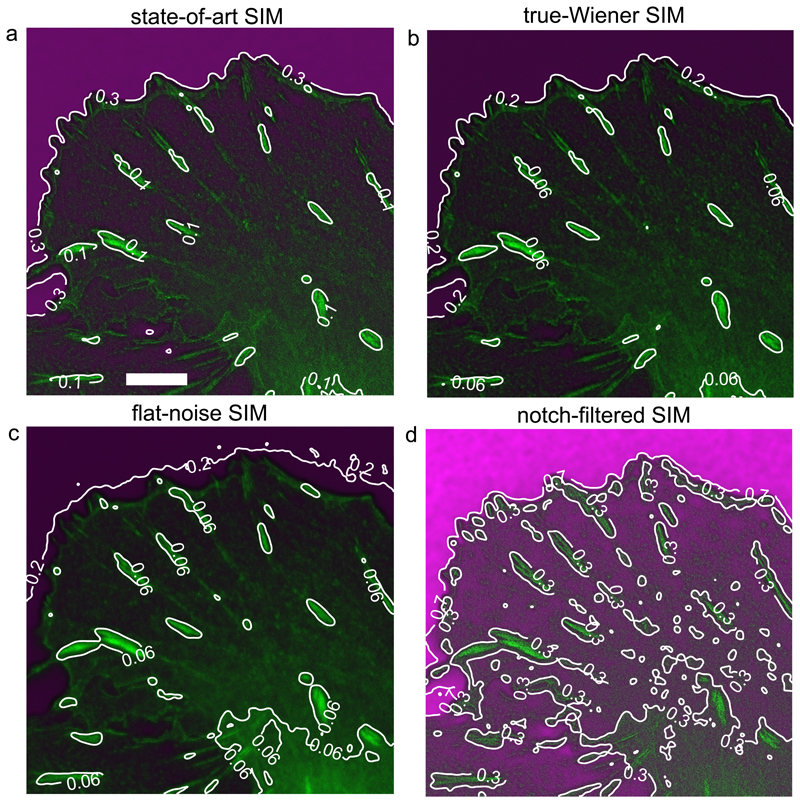
Extended Data Figure 1
Noise-controlled SIM reconstructions of GFP-zyxin protein in focal adhesions (green) and noise fraction map (magenta) over full FOV.
(a-d) State-of-art SIM ( w = 5 u00d7 10 u22124 ), true-Wiener SIM, flat-noise SIM, and notch-filtered SIM reconstructions. Contours of the noise fraction map are added in white with contour level indi...
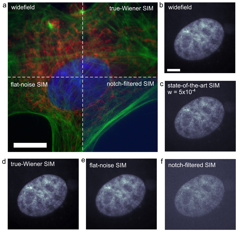
Extended Data Figure 2
Multi-colour noise-controlled 2D SIM reconstructions.
(a) Combined widefield, true-Wiener SIM, flat-noise SIM, and notch-filtered SIM reconstructions of a fluorescent test slide of a bovine pulmonary artery endothelial cell (red channel: mitochondria lab...
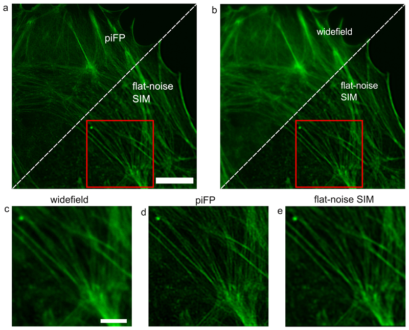
Extended Data Figure 3
Noise propagation in DMD-SIM.
(a) Reconstructions of Alexa Fluor 488 labelled actin filaments in a bovine pulmonary artery endothelial cell with the iterative pattern-illuminated Fourier Ptychography (piFP) algorithm (see Suppleme...
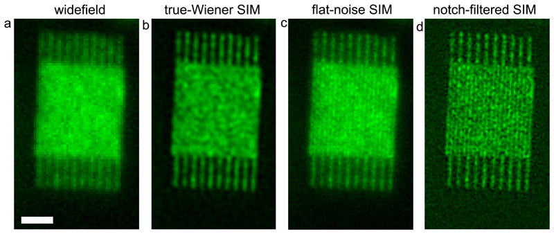
Extended Data Figure 4
Flat-noise SIM provides better visibility of high spatial frequency structures.
(a-d) Widefield, true-Wiener, flat-noise, and notch-filtered SIM reconstructions of a nano-fabricated test structure of lines with 140 nm pitch. The line pattern is just visible in flat-noise, and not...
Extended Data Figure 5
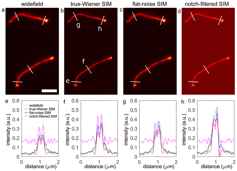
Noise-controlled 2D SIM of synaptonemal complex.
(a-d) Widefield, and true-Wiener, flat-noise and notch-filtered SIM reconstructions of the mCherry-CSYCP3 protein in the synaptonemal complex. (e-h) Line profiles along the lines indicated in (b) . Th...
Extended Data Figure 6
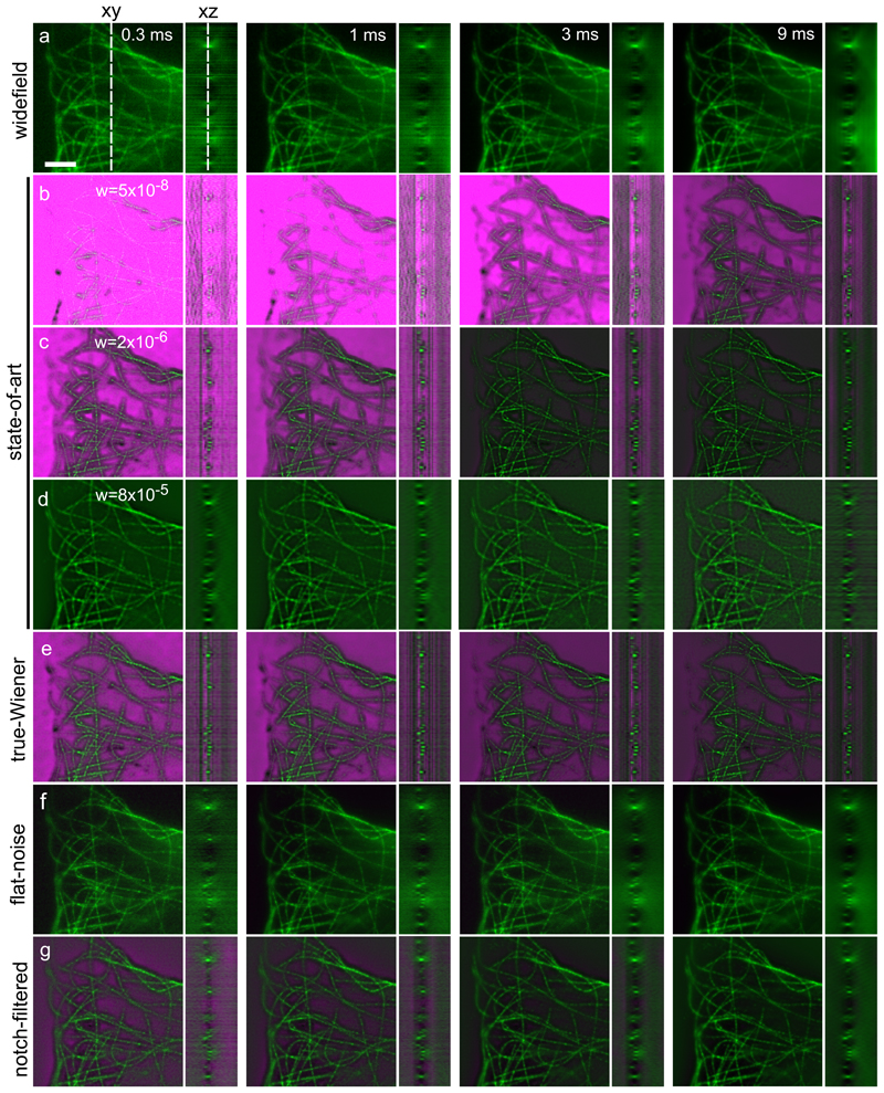
Cross-sections in xy and yz-planes of 3D-reconstructions of tubulin (green) and noise fraction maps (magenta) for different camera exposure times.
(a) Widefield, (b-d) state-of-the-art SIM for low, medium and high regularization, (e) true-Wiener SIM, (f) flat-noise SIM, and (g) notch-filtered SIM. The dashed lines in (a) indicate the location of...
Extended Data Figure 7
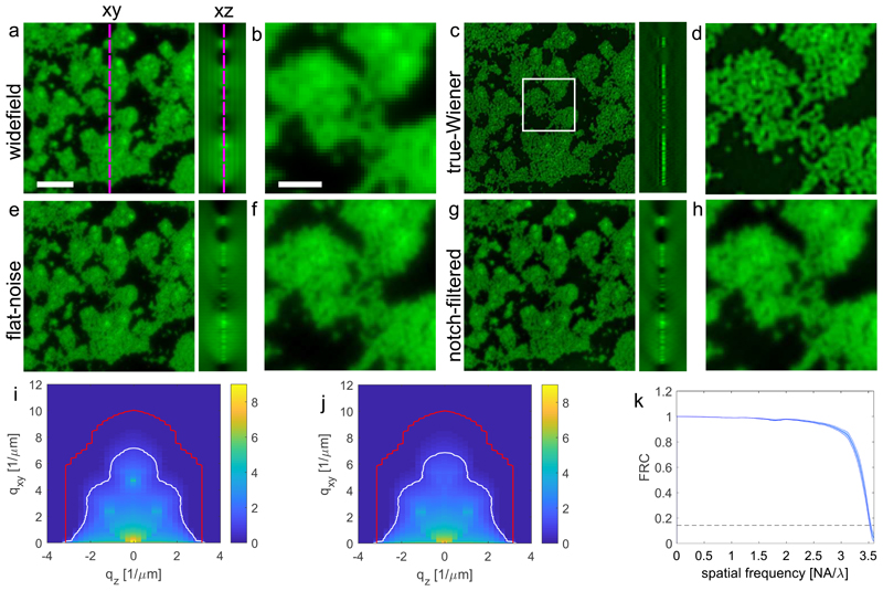
Widefield and noise-controlled 3D-SIM reconstructions of a 100 nm bead layer sample.
(a,b) Widefield, (c,d) true-Wiener SIM, (e,f) flat-noise SIM, (g,h) notch-filtered SIM. The white box in (c) indicates the insets (b,d,f,h) . (i,j) SSNR of the SIM reconstructions without (i) and with...
Extended Data Figure 8
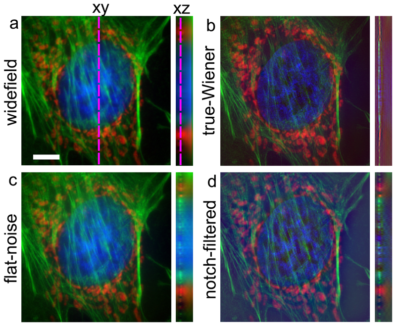
Widefield and 3D noise-controlled SIM reconstructions of a bovine pulmonary artery endothelial cell.
(a) Widefield, (b) true-Wiener SIM, (c) flat-noise SIM, (d) notch-filtered SIM (BPAEC, red channel: mitochondria labelled with Alexa Fluor 594, green channel: actin labelled with FITC, blue channel: D...
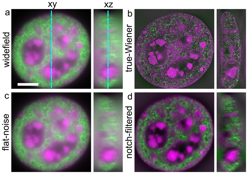
Extended Data Figure 9
Widefield and 3D noise-controlled SIM reconstructions of a mouse C127 cell.
(a) Widefield, (b) true-Wiener SIM, (c) flat-noise SIM, (d) notch-filtered SIM (magenta channel: DNA labelled with DAPI, green channel: H3K4me3 labelled with Alexa Fluor 488, blue channel: DNA labelle...
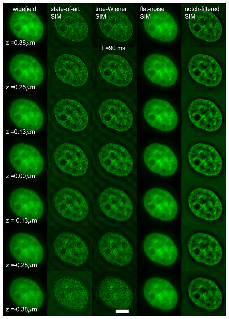
Extended Data Figure 10
Widefield, state-of-the-art SIM and noise-controlled 3D-SIM reconstructions for one time frame of the 15 time-frame, 7-layer dataset of H2B-GFP histone in a live HeLa cell. Scale bar 6 u03bcm.
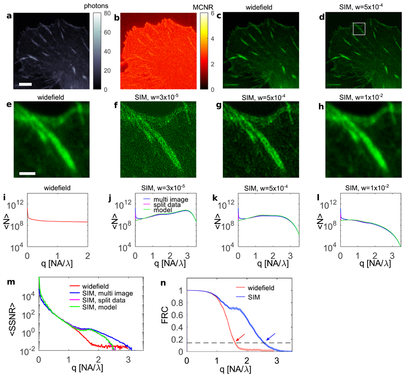
Figure 1
Noise propagation in SIM reconstructions.
( a ) Example raw image of a SIM acquisition of GFP-zyxin in focal adhesions, and ( b ) Modulation Contrast to Noise Ratio (MCNR), indicating muted stripe contrast due to low signal levels. ( c-d ) Wi...
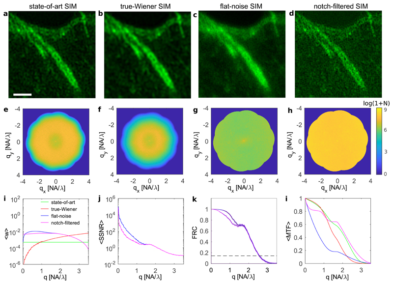
Figure 2
Noise controlled SIM reconstructions.
( a ) State-of-the-art SIM with regularization w = 5 u00d7 10 u22124 ( b ) True-Wiener SIM, ( c ) flat-noise SIM, and ( d ) notch-filtered SIM reconstructions for the inset shown in Fig. 1e-h . The tw...
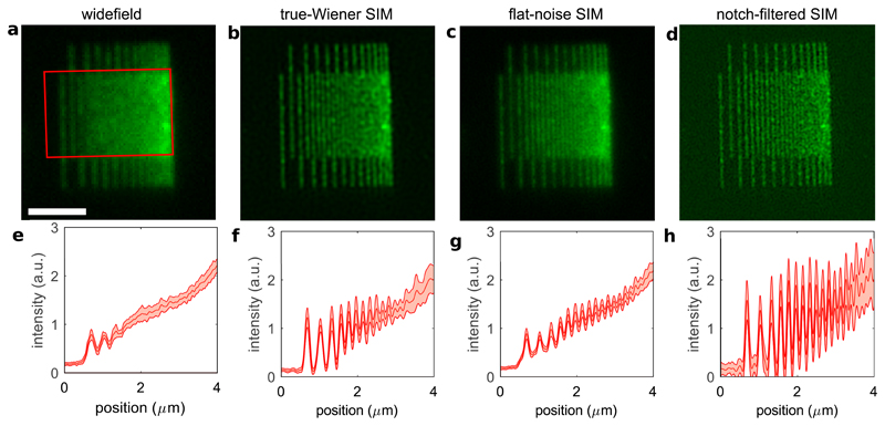
Figure 3
Trade-off between noise and contrast in SIM reconstructions.
( a-d ) Widefield and the three noise-controlled SIM reconstruction of a chirped nano-patterned structure. ( e-h ) Mean and standard deviation of the chirped line pattern over the boxed region in a fo...
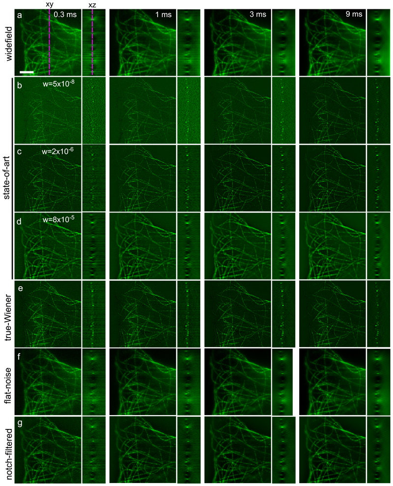
Figure 4
Noise-controlled 3D SIM reconstructions.
Cross-sections of 3D-reconstructions ( xy and yz ) for four different signal levels (camera exposure indicated) ( a ) widefield, ( b-d ) state-of-the-art SIM for low, medium and high regularization, (...
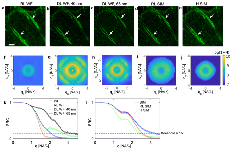
Figure 5
Resolution improvement and noise enhancement in deconvolution of GFP-zyxin dataset.
(a) RL-deconvolution of widefield image, (b) DL-deconvolution of widefield image at 40 nm pixel size, (c) DL-deconvolution of widefield image at 65 nm pixel size, (d) RL-deconvolution of (flat-noise) ...
Figure images are served from the NIH/NLM PubMed Central Open Access Subset or Europe PMC; copyright remains with the publishers and authors.
💬 Discussion
0 commentsNo comments yet. Be the first to start a discussion!
Leave a Comment