Abstract
Deposits of amyloid fibrils of α-synuclein are the histological hallmarks of Parkinson's disease, dementia with Lewy bodies and multiple system atrophy, with hereditary mutations in α-synuclein linked to the first two of these conditions. Seeing the changes to the structures of amyloid fibrils bearing these mutations may help to understand these diseases. To this end, we determined the cryo-EM structures of α-synuclein fibrils containing the H50Q hereditary mutation. We find that the H50Q mutation results in two previously unobserved polymorphs of α-synuclein: narrow and wide fibrils, formed from either one or two protofilaments, respectively. These structures recapitulate conserved features of the wild-type fold but reveal new structural elements, including a previously unobserved hydrogen-bond network and surprising new protofilament arrangements. The structures of the H50Q polymorphs help to rationalize the faster aggregation kinetics, higher seeding capacity in biosensor cells and greater cytotoxicity that we observe for H50Q compared to wild-type α-synuclein.
🔬 Techniques
🔭 Microscopes
💻 Software
✨ Fluorophores
🧪 Sample Preparation
🔬 Cell Lines
🏭 Microscope Brands
🧪 Reagent Suppliers
📷 Detectors
💻 Software Details
💾 Data Repositories
🏛️ Research Organizations (ROR)
Affiliated research institutions:
📋 Methods
Protein purification
Full-length aSyn WT and H50Q mutant proteins were expressed and purified according to a published protocol 14 . The bacterial induction started at an OD600 of ~0.6 with 1 mM IPTG for 6 h at 30°C. The harvested bacteria were lysed with a probe sonicator for 10 minutes in an iced water bath. After centrifugation, the soluble fraction was heated in boiling water for 10 minutes and then titrated with HCl to pH 4.5 to remove the unwanted precipitants. After adjusting to neutral pH, the protein was dialyzed overnight against Q Column loading buffer (20 mM Tris-HCl, pH 8.0). On the next day, the protein was loaded onto a HiPrep Q 16/10 column and eluted using elution buffer (20 mM Tris-HCl, 1M NaCl, pH 8.0). The eluent was concentrated using Amicon Ultra-15 centrifugal filters (Millipore Sigma) to ~5 mL. The concentrated sample was further purified with size-exclusion chromatography through a HiPrep Sephacryl S-75 HR column in 20 mM Tris, pH 8.0. The purified protein was dialyzed against water, concentrated to 3 mg/ml, and stored at 4C. The concentration of the protein was determined using the Pierce™ BCA Protein Assay Kit (cat. No. 23225, Thermo Fisher Scientific). Fibril preparation and optimization Both WT and H50Q fibrils were grown under the same condition: 300 μM purified monomers, 15mM tetrabutylphosphonium bromide, shaking at 37°C for 2 weeks. Negative stain transmission electron microscopy (TEM) The fibril sample (3 μL) was spotted onto a freshly glow-discharged carbon-coated electron microscopy grid. After 1 minute, 6 μL uranyl acetate (2% in aqueous solution) was applied to the grid for 1 minutes. The excessive stain was remove by a filter paper. Another 6μL uranyl acetate was applied to the grid and immediately removed. The samples were imaged using an FEI T20 electron microscope. Thioflavin-T binding assay 50 μM of purified aSyn monomers were adequately mixed with 20 μM thioflavin T and added into a 96-well-plate. Samples were incubated at 37°C for 2 days with 600 rpm double orbital shaking. The ThT signal was monitored using the FLUOstar Omega Microplate Reader (BMG Labtech; Cary, NC) at an excitation wavelength of 440 nm and an emission wavelength of 490 nm. SDS Stability SDS was diluted in water to make SDS solutions at 2.5%, 5%, 10% and 15%. Fibrils at the end of the ThT assay were treated with SDS solution at 5:1 volume ratio to obtain SDS concentrations of 0.5%, 1%, 2% and 3%. Each solution was transferred to 3 microcentrifuge tubes and heated at 70° C for 15 minutes. After the treatment, the ThT signal was obtained. The 0% SDS solution without heating was treated with equal amount of water and used for normalization.
Show full methods section
Protein purification
Full-length aSyn WT and H50Q mutant proteins were expressed and purified according to a published protocol 14 . The bacterial induction started at an OD600 of ~0.6 with 1 mM IPTG for 6 h at 30°C. The harvested bacteria were lysed with a probe sonicator for 10 minutes in an iced water bath. After centrifugation, the soluble fraction was heated in boiling water for 10 minutes and then titrated with HCl to pH 4.5 to remove the unwanted precipitants. After adjusting to neutral pH, the protein was dialyzed overnight against Q Column loading buffer (20 mM Tris-HCl, pH 8.0). On the next day, the protein was loaded onto a HiPrep Q 16/10 column and eluted using elution buffer (20 mM Tris-HCl, 1M NaCl, pH 8.0). The eluent was concentrated using Amicon Ultra-15 centrifugal filters (Millipore Sigma) to ~5 mL. The concentrated sample was further purified with size-exclusion chromatography through a HiPrep Sephacryl S-75 HR column in 20 mM Tris, pH 8.0. The purified protein was dialyzed against water, concentrated to 3 mg/ml, and stored at 4C. The concentration of the protein was determined using the Pierce™ BCA Protein Assay Kit (cat. No. 23225, Thermo Fisher Scientific). Fibril preparation and optimization Both WT and H50Q fibrils were grown under the same condition: 300 μM purified monomers, 15mM tetrabutylphosphonium bromide, shaking at 37°C for 2 weeks. Negative stain transmission electron microscopy (TEM) The fibril sample (3 μL) was spotted onto a freshly glow-discharged carbon-coated electron microscopy grid. After 1 minute, 6 μL uranyl acetate (2% in aqueous solution) was applied to the grid for 1 minutes. The excessive stain was remove by a filter paper. Another 6μL uranyl acetate was applied to the grid and immediately removed. The samples were imaged using an FEI T20 electron microscope. Thioflavin-T binding assay 50 μM of purified aSyn monomers were adequately mixed with 20 μM thioflavin T and added into a 96-well-plate. Samples were incubated at 37°C for 2 days with 600 rpm double orbital shaking. The ThT signal was monitored using the FLUOstar Omega Microplate Reader (BMG Labtech; Cary, NC) at an excitation wavelength of 440 nm and an emission wavelength of 490 nm. SDS Stability SDS was diluted in water to make SDS solutions at 2.5%, 5%, 10% and 15%. Fibrils at the end of the ThT assay were treated with SDS solution at 5:1 volume ratio to obtain SDS concentrations of 0.5%, 1%, 2% and 3%. Each solution was transferred to 3 microcentrifuge tubes and heated at 70° C for 15 minutes. After the treatment, the ThT signal was obtained. The 0% SDS solution without heating was treated with equal amount of water and used for normalization.
Cell Lines
HEK293T biosensor cells expressing α-syn-A53T-YFP were a generous gift from the lab of Dr. Marc Diamond. PC12 cells originate from the ATCC (ATCC® CRL-1721™). Cells were not authenticated nor tested for mycoplasma infection in our hands.
Fibril seeding aggregation in cells
We performed the biosensor cell seeding assay based on a previously published protocol 26 . Briefly, the assay works as follows: exogenous, un-labeled fibrils are transfected into HEK293T cells expressing α-syn-A53T-YFP. Seeded aggregation of endogenously expressed α-syn-A53T-YFP is monitored by formation of fluorescent puncta. The puncta represent a condensation of α-syn-A53T-YFP as a result of seeding by exogenous H50Q or WT fibrils.
Human embryonic kidney FRET Biosensor
HEK293T cells expressing full-length aSyn containing the hereditary A53T mutation were grown in DMEM (4mM L-glutamine and 25mM D-glucose) supplemented with 10% FBS, 1% penicillin/streptomycin. Trypsin-treated HEK293T cells were harvested, seeded on flat 96-well plates at a concentration of 4×10⁴ cells/well in 200 μL culture medium per well and incubated in 5% CO2 at 37°C for 18 hours. aSyn fibrils were prepared by diluting with Opti-MEM™ (Life Technologies; Carlsbad CA) and sonicating in a water bath sonicator for 10 minutes. The fibril samples were then mixed with Lipofectamine™ 2000 (Thermo Fisher Scientific) and incubated for 15 minutes and then added to the cells. The actual volume of Lipofectamine™ 2000 was calculated based on the dose of 1 μL per well. After 48 hours of transfection, the cells were trypsinized, transferred to a 96-well round-bottom plate and resuspended in 200 μL chilled flow cytometry buffer (HBSS, 1% FBS, and 1 mM EDTA) containing 2% paraformaldehyde. The plate was sealed with Parafilm and stored at 4 °C for imaging. Fluorescent images were processed in ImageJ to count number of seeded cells.
MTT mitochondrial activity assay
The addition of sonicated fibrils to Nerve Growth Factor-differentiated PC12 cells is a well-established assay to measure cytotoxicity of amyloid fibrils 40 , 41 . Use of this neuron-like cell line allows us to obtain a biologically relevant assay for cytotoxicity. For our MTT mitochondrial activity assay, the protocol was adapted from the Provost and Wallert laboratories 42 . Thiazolyl blue tetrazolium bromide for the MTT cell toxicity assay was purchased from Millipore Sigma (M2128-1G; Burlington, MA). PC12 cells were plated in 96-well plates at 10,000 cells/well in DMEM (Dulbecco’s modification of Eagle’s medium; 5% fetal bovine serum [FBS], 5% heat-inactivated horse serum, 1% penicillin/streptomycin and 150 ng/mL nerve growth factor 2.5S (Thermo Fisher Scientific). The cells were incubated for 2 days in an incubator with 5% CO2 at 37°C. The cells were treated with different concentrations of aSyn fibrils (200 nM, 500 nM,1000 nM, 2000 nM). After 18 hours of incubation, 20 μl of 5 mg/ml MTT was added to every well and the plate was returned to the incubator for 3.5 hours. With the presence of MTT, the experiment was conducted in a laminar flow hood with the lights off and the plate was wrapped in aluminum foil. The media was then removed with an aspirator and the remained formazan crystals in each well were dissolved with 100 μL of 100% DMSO. Absorbance was measured at 570 nm to determine the MTT signal and at 630 nm to determine background. The data were normalized to those from cells treated with 1% SDS to obtain a value of 0%, and to those from cells treated with PBS to obtain a value of 100%. Lactate Dehydrogenase (LDH) Assay The LDH viability assay was performed using the CytoTox-ONE™ Homogeneous Membrane Integrity Assay (Promega; Madison, WI, G7891). PC12 cells were cultured and differentiated with the same protocol as described in the MTT assay. Different concentrations of aSyn fibrils (200 nM, 500 nM, 1000 nM, 2000nM) were added to the cells for 18 hours of incubation with 5% CO2 at 37°C. The assay was carried out in a 96 well plate and the fluorescent readings were taken in the FLUOstar Omega Microplate Reader (Ex. 560 nm, Em. 590 nm, BMGLabtech; Cary, NC). PBS and 0.2% Triton-X100 treated cells were used as negative and positive control for normalization. Cryo-EM data collection and processing 2 μl of fibril solution was applied to a baked and glow-discharged Quantifoil 1.2/1.3 electron microscope grid and plunge-frozen into liquid ethane using a Vitrobot Mark IV (FEI). Data were collected on a Titan Krios (FEI) microscope equipped with a Gatan Quantum LS/K2 Summit direct electron detection camera (operated with 300 kV acceleration voltage and slit width of 20 eV). Counting mode movies were collected on a Gatan K2 Summit direct electron detector with a nominal physical pixel size of 1.07 Å/pixel with a dose per frame 1.2 e-/Å 2 . A total of 30 frames with a frame rate of 5 Hz were taken for each movie resulting in a final dose 36 e-/Å 2 per image. Automated data collection was driven by the Leginon automation software package 43 . Micrographs containing crystalline ice were used to estimate the anisotropic magnification distortion using mag_distortion_estimate 44 . CTF estimation was performed using CTFFIND 4.1.8 on movie stacks with a grouping of 3 frames and correction for anisotropic magnification distortion 45 . Unblur 46 was used to correct beam-induced motion with dose weighting and anisotropic magnification correction, resulting in a physical pixel size of 1.065 Å/pixel. All particle picking was performed manually using EMAN2 e2helixboxer.py 47 . We manually picked two groups of particles for further data processing: the first group was composed of all fibrils and the second group was composed of Wide Fibrils. For the first group, particles were extracted in RELION using the 90% overlap scheme into 1024 and 288 pixel boxes. Classification, helical reconstruction, and 3D refinement were used in RELION as described 48 . For the first group of all particles, we isolated Narrow Fibrils during 2D Classification and subsequently processed them as a separate data set. 2D Classifications of Narrow Fibril 1024 pixel boxes were used to estimate helical parameters. We performed 3D classification with the estimated helical parameters for Narrow Fibrils and an elongated Gaussian blob as an initial model to generate starting reconstructions. We ran additional 3D classifications using the preliminary reconstructions from the previous step to select for particles contributing to homogenous classes (stable helicity and separation of β-strands in the X-Y plane). Typically, we performed Class3D jobs with K=3 and manual control of the tau_fudge factor and healpix to reach a resolution of ~5-6 Å to select for particles that contributed to the highest resolution class for each structure. We employed Refine3D on a final subset of Narrow Fibril particles with 288 pixel box size to obtain the final reconstruction. We performed the map-map FSC with a generous, soft-edged solvent mask and high-resolution noise substitution in RELION PostProcess resulting in a resolution estimate of 3.3 Å. We extracted particles from the Wide Fibril data set using 1024 and 686 pixel boxes. 2D Classifications of 1024 and 686 pixel boxes were used to estimate helical parameters. 2D Classifications of 686 pixel boxes were used to further isolate only Wide Fibril segments since there was still some other fibril species that were included due to the fact that we could not separate all fibril species perfectly during manual picking. Once a homogenous set of Wide Fibrils was obtained during 2D Classification of 686 pixel boxes, we performed a 3D reconstruction using an elongated Gaussian blob as an initial model. The asymmetry present in the 686 box 2D class averages of the Wide Fibril ( Extended Data Figure 2 d ) prompted us to use a helical rise of 4.8 Å and C1 symmetry due to the fact that if a 2-fold symmetry were present in the fibrils, 2D class averages would display a mirror symmetry across the fibril axis. After an initial 2D model was generated for the Wide Fibril, we re-extracted all tubes corresponding to those particles included in the final subset of Wide Fibril 686 pixel boxes with a box size of 224 pixels. All 224 pixel boxes were subjected to multiple rounds of 3D Classification using the initial 686 pixel box Wide Fibril reconstruction as a reference. We refined the final subset of particles using Refine3D to a resolution of 3.6 Å. We performed resolution estimation as described above for the Narrow Fibrils. Atomic model building We sharpened both the Narrow and Wide Fibril reconstructions using phenix.auto_sharpen 49 at the resolution cutoff indicated by the map-map FSC and subsequently built atomic models in to the refined maps with COOT 50 . We built the model for the Narrow Fibril de novo using previous structures of wild-type alphα-synuclein fibrils as guides. To build the Wide Fibril model, we made a copy of one chain of the Narrow Fibril structure and rigid-body fit it into the second protofilament density observed in the Wide Fibril reconstruction. This resulted in the Wide Fibril being composed of one protofilament nearly identical to the Narrow Fibril and one protofilament with less ordered N- and C-termini, therefore resulting in an asymmetric double protofilament structure. For both Narrow and Wide Fibrils, we generated a 5-layer model to maintain local contacts between chains in the fibril during structure refinement. We performed automated structure refinement for both Narrow and Wide Fibrils using phenix.real_space_refine 51 . We employed hydrogen bond distance and angle restraints for backbone atoms participating in β-sheets and side chain hydrogen bonds during automated refinements. We performed comprehensive structure validation of all our final models in Phenix. Although we did not include coordinates in our final models for additional residues that could occupy Islands 1 and 2 neighboring Protofilament A because we could not be certain which residues occupy those densities, we built several speculative models ( Extended Data Figure 4 ). For Island 2, we assumed that there was a short disordered linker between residue 36 of Protofilament A and Island 2 resulting in the residues occupying Island 2 forming a tight interface with 36 GVLYVG 41 of the fibril core. We noticed that the sequence 32 KTKE 35 immediately precedes the last ordered residue of Protofilament A, G36. 32 KTKE 35 often forms the bends that connect straight β-strands in the ordered fibril core, so we assumed that this sequence would be a good candidate to form the tight bend that connects G36 to Island 2. Therefore, we modeled in residues 26 VAEAAG 31 into Island 2. These residues satisfied the requirements of having short, hydrophobic side chains forming the tight interface with residues V38 and L40 from the fibril core. For Island 1, we assumed the densities either come from the N-terminus of Protofilament A or the C-terminus of Protofilament B. For the former case, we assume that there is a minimum of ~8 residues that are disordered between the end of Island 2 and the beginning of Island 1 (see Extended Data Figure 4 ). This is because there is 27 Å between the end of Island 2 - V26 - and the beginning of Island 1, and we assume a minimum of ~3.3 Å/residue. Therefore, we threaded 8 residues at a time from the region 1 MDVFMKGLSKAKEGVVAAA 20 onto a β-strand backbone placed in the Island 1 density to identify candidate 8mers. While most sequences could not plausibly occupy Island 1 due to steric clashes with the preNAC region of the fibril core, or due to glycine residues occupying positions where there were obvious side chain densities, several candidate sequences were identified ( Extended Data Figure 3 ). We followed a similar protocol to identify possible sequences from the C-terminus. In this case, we assume that these residues could come from either a largely disordered Protofilament B molecule in the Narrow Fibril or an ordered Protofilament B molecule as seen in the Wide Fibril (see Extended Data Figure 3 ). Here, we assume there is a minimum of ~15 residues from the last ordered residue of the C-terminus of Protofilament B - since we assume a minimum of ~3.3 Å/residue and there is ~45 Å between K97 of Protofilament B and the beginning of Island 1 (see Extended Data Figure 3 ). Therefore, we threaded all possible 8mers from the region 112 ILEDMPVDPDNEAYEMPSEEGYQDYEPEA 140 onto a β-strand backbone occupying Island 1 to identify candidate sequences following the same criterion as above. We created the speculative model of an H50Q double protofilament containing a homomeric preNAC interface by aligning a single chain from the H50Q Narrow Protofilament with the helical axis of the wild-type “rod” structure (6CU7) and applying a pseudo-2(1) helical symmetry to generate a symmetrically related second chain. Energetic calculation The stabilization energy is an adaptation of the solvation free energy described previously 52 , in which the energy is calculated as the sum of products of the area buried of each atom and its corresponding atomic solvation parameter (ASP). ASPs were taken from our previous work 52 . Area buried is calculated as the difference in solvent accessible surface area (SASA) of the reference state (i.e. unfolded state) and the SASA of the folded state. The reference state was measured absent all other atoms in the structure but the residue “i” and main chain atoms of residue i-1 and i+1. The SASA of the folded state was measured for each atom in the context of all amyloid fibril atoms. Fibril coordinates were extended by symmetry by three to five chains on either side of the reported molecule, to ensure the energetic calculations were representative of the majority of molecules in a fibril, rather than a fibril end. To account for energetic stabilization of main chain hydrogen bonds, the ASP for backbone N/O elements was reassigned from −9 to 0 if they participated in a hydrogen bond. Similarly, if an asparagine or glutamine side chain participated in a polar ladder (two hydrogen bonds per amide), and was shielded from solvent (SASAfolded < 5 Å 2 ), the ASPs of the side chain N and O elements were reassigned from −9 to 0. Lastly, the ASP of ionizable atoms (e.g. Asp, Glu, Lys, His, Arg, N-terminal amine, or C-terminal carboxylate) were assigned the charged value (−37/−38) unless the atoms participated in a buried ion pair, defined as a pair of complementary ionizable atoms within 4.2 Å distance of each other, each with SASAfolded < 40 Å 2 ). In that case, the ASP of the ion pair was reassigned to −9. In the energy diagrams, a single color is assigned to each residue, rather than each atom. The color corresponds to the sum of solvation free energy values of each of the atoms in the residue. The energy reported for FUS in Table 2 is the average over 20 NMR models. The standard deviation is 1.8 kcal/mol. Data Availability Statement: All structural data have been deposited into the wwPDB and EMDB with the following accession codes: H50Q Narrow Fibril (PDB 6PEO, EMD-20328) and H50Q Wide Fibril (PDB 6PES, EMD-20331). All other data are available from the authors upon reasonable request. Reporting Summary Statement: Further information on experimental design is available in the Nature Research Reporting Summary linked to this article.
Supplementary Material 1
📊 Figures
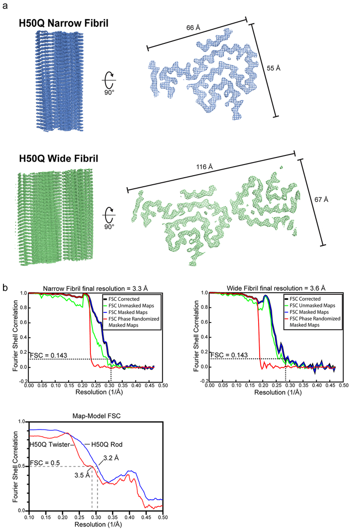
Extended Data Fig. 1
Fourier Shell Analysis
a) Helical reconstructions of Narrow and Wide Fibrils with minimum and maximum widths labeled. b) Gold-standard half map FSC curves for Narrow (top, left) and Wide (top, right) Fibrils. Map-model FSC ...
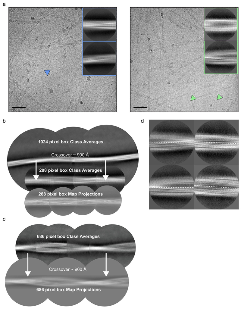
Extended Data Fig. 2
Cryo-EM images and processing
a) Cryo-EM micrographs and 2D class averages of Narrow (left) and Wide (right) Fibrils. Scale bar = 50 nm. b) 1024 and 288 pixel box size class averages of the Narrow Fibril used to determine crossove...
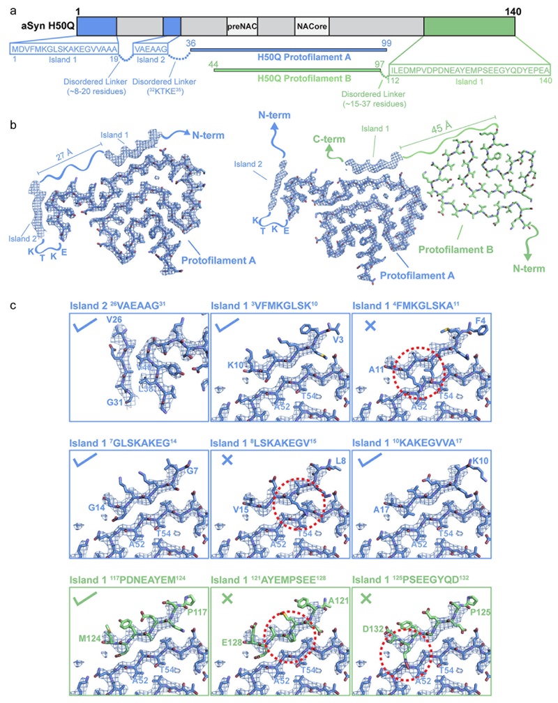
Extended Data Fig. 3
Speculative Atomic Models for Islands 1 and 2
a) Schematic illustrating possible sequences occupying Islands 1 and 2. 8mers from residues 1-19 and 112-140 were considered as possibilities to occupy Island 1. Island 2 is considered to consist of r...
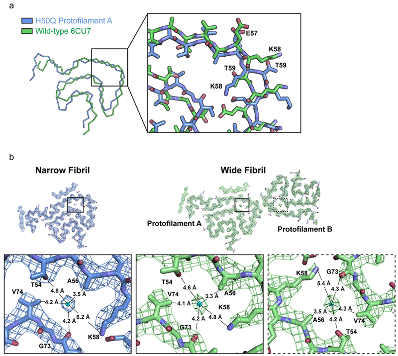
Extended Data Fig. 4
Alternate conformations of K58 and T59 and potential solvent molecules in the u03b1-syn u03b2-arch cavity
a) Wild-type and H50Q fibrils display alternate conformations of K58 and T59. We note that in order for the Wide Fibril to form, T59 needs to be facing away from the fibril core. Therefore the formati...
Extended Data Fig. 5
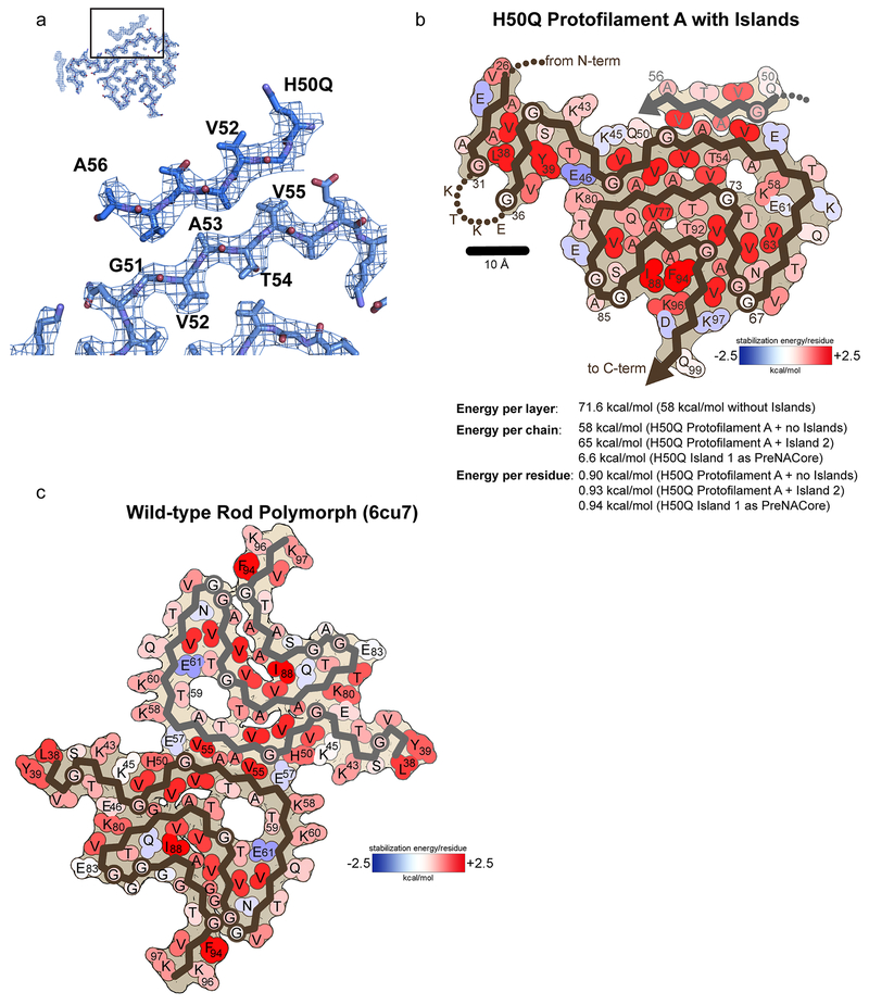
PreNAC homozipper Island 1 model and additional solvation energy maps
a) Speculative model of preNAC residues 50 QGVATVA 56 occupying Island 1 in Protofilament A. b) Atomic solvation map and energetic calculations for Protofilament A with Island 1 as 50 QGVATVA 56 and I...
Extended Data Fig. 6
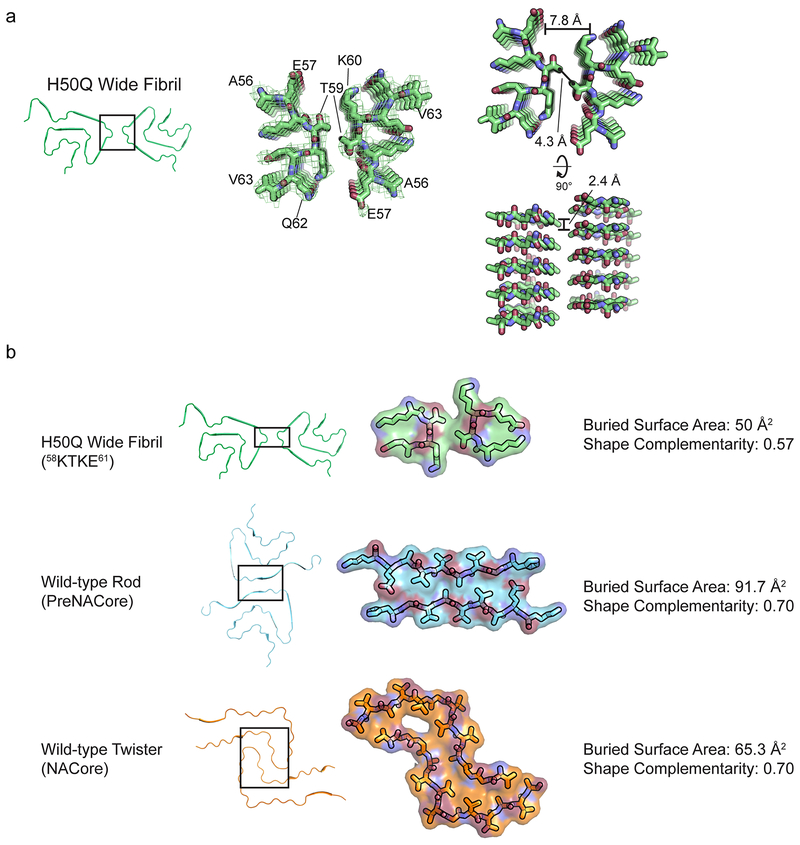
Comparison of u03b1-syn protofilament interfaces
a) Wide Fibril overview (left). 56 AEKTKEQV 63 homointerface with Wide Fibril electron density (middle). 56 AEKTKEQV 63 homointerface showing a 2.4 u00c5 rise between mated strands from Protofilament ...
Extended Data Fig. 7
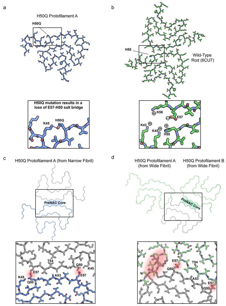
H50Q disrupts the wild-type rod polymorph preNAC protofilament interface
a) Conformation of H50Q Protofilament A K45 and H50Q. b) Interaction of K45-H50-E57 in the wild-type rod polymorph protofilament interface. c) Hypothetical H50Q double protofilament using the preNAC o...

Extended Data Fig. 8
H50Q fibrils disrupt PC12 cell membranes more than WT fibrils
Differentiated PC12 cells were treated with sonicated WT and H50Q fibrils and cell permeability was measured via LDH activity in the media (see Methods). H50Q leads to significantly higher cell permea...
Extended Data Fig. 9
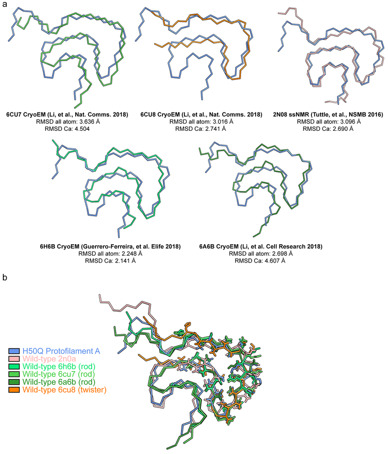
Structural alignment of different wild-type and mutant u03b1-syn polymorphs
a) Structural alignment of H50Q Protofilament A with all wild-type structures determined thus far. b) Structural alignment of residues 50-57 in wild-type and mutant u03b1-syn polymorphs reveals the ke...
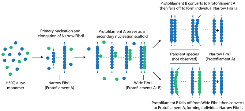
Extended Data Fig. 10
Schematic illustrating possible secondary nucleation of Protofilament B by Narrow Fibrils
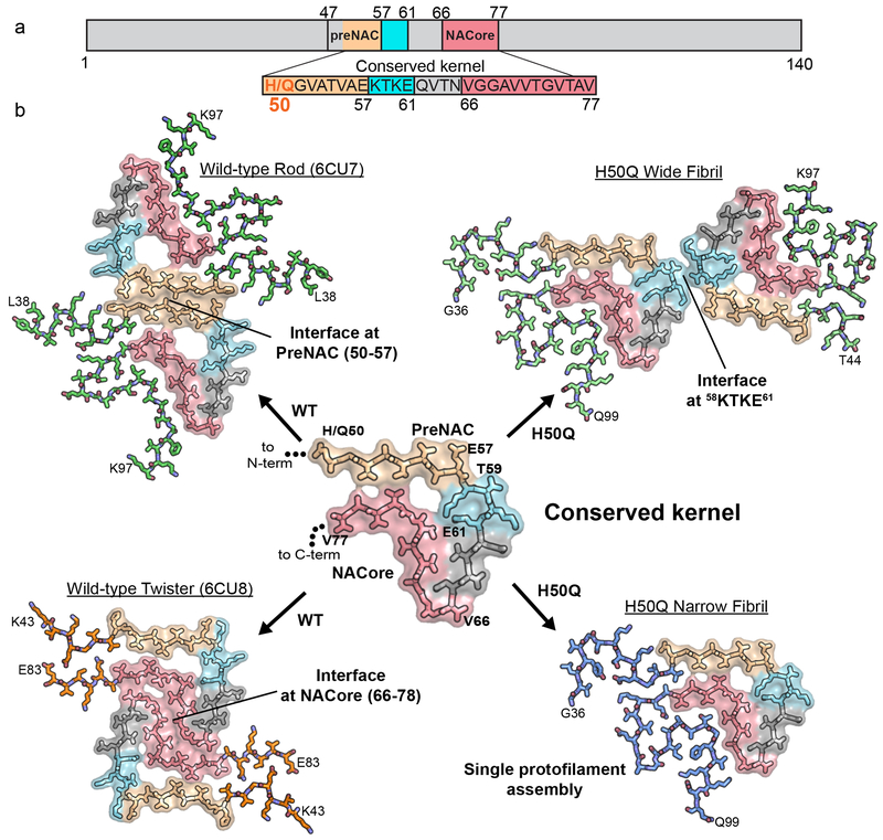
Figure 1
Comparison of wild-type and H50Q polymorphs. a) Primary structure schematic highlighting residues of the conserved kernel (50u201377) that are used as protofilament interfaces in u03b1-syn polymorphs....
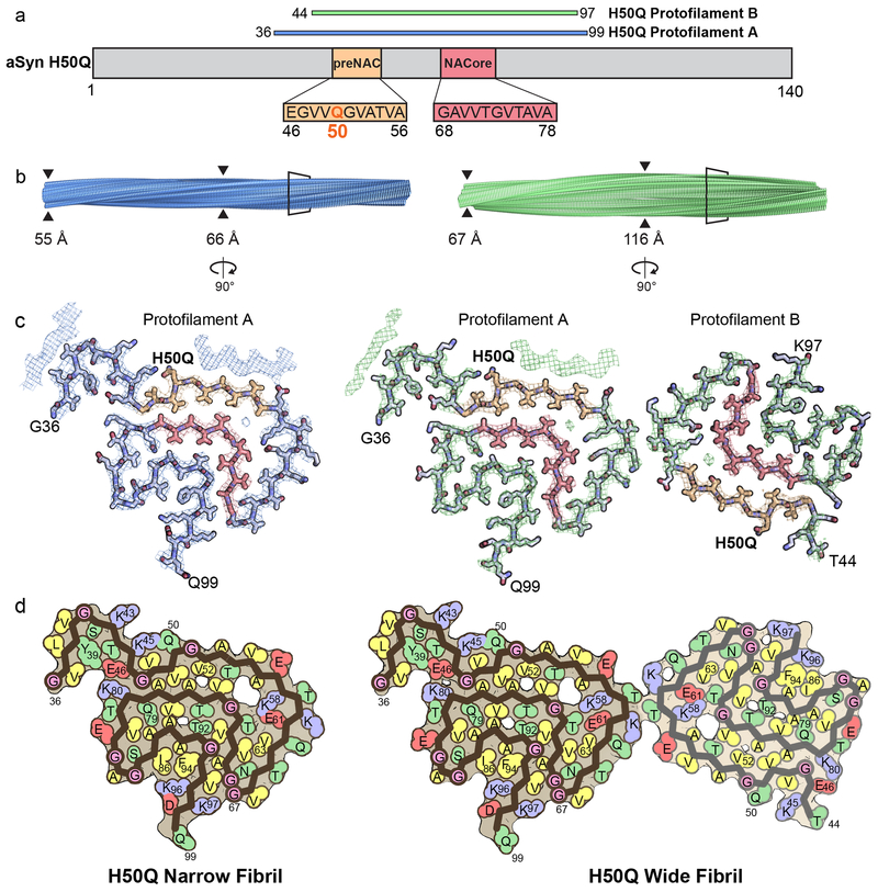
Figure 2
Cryo-EM Structures of H50Q Polymorphs a) Schematic of u03b1-syn primary structure demonstrating location of the ordered core of H50Q Protofilaments A and B, preNAC and NACore, and H50Q hereditary muta...
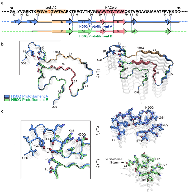
Figure 3.
Comparison of Protofilaments A and B a) Schematic of primary and secondary structure of fibril core of H50Q Protofilaments A and B. Arrows indicate regions of Protofilaments A and B that adopt u03b2-s...
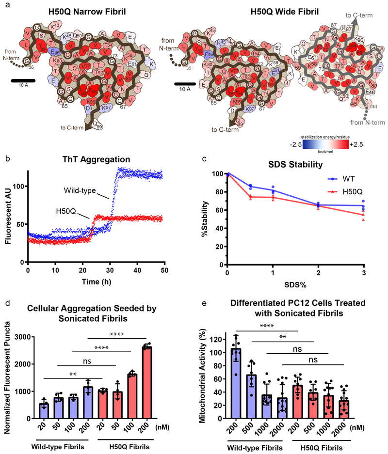
Figure 4.
Solvation energy maps and biochemical characterization of H50Q and wild-type u03b1-syn. a) Solvation energy maps of H50Q Narrow and Wide Fibrils. The stabilizing residues are red; the de-stabilizing r...
Figure images are served from the NIH/NLM PubMed Central Open Access Subset or Europe PMC; copyright remains with the publishers and authors.
💬 Discussion
0 commentsNo comments yet. Be the first to start a discussion!
Leave a Comment