Abstract
Abstract The axial resolution of three-dimensional structured illumination microscopy (3D SIM) is limited to ∼300 nm. Here we present two distinct, complementary methods to improve axial resolution in 3D SIM with minimal or no modification to the optical system. We show that placing a mirror directly opposite the sample enables four-beam interference with higher spatial frequency content than 3D SIM illumination, offering near-isotropic imaging with ∼120-nm lateral and 160-nm axial resolution. We also developed a deep learning method achieving ∼120-nm isotropic resolution. This method can be combined with denoising to facilitate volumetric imaging spanning dozens of timepoints. We demonstrate the potential of these advances by imaging a variety of cellular samples, delineating the nanoscale distribution of vimentin and microtubule filaments, observing the relative positions of caveolar coat proteins and lysosomal markers and visualizing cytoskeletal dynamics within T cells in the early stages of immune synapse formation.
🔬 Techniques
✨ Fluorophores
🧪 Sample Preparation
🔬 Cell Lines
🏭 Microscope Brands
🧪 Reagent Suppliers
📷 Detectors
🎨 Filters
💻 Software Details
💻 Code & Software
code of the registration and deconvolution project
Image restoration for fluorescence microscopy
Three-dimensional residual channel attention networks
💾 Data Repositories
🏛️ Research Organizations (ROR)
Affiliated research institutions:
📋 Methods
Simulations of OTF support The simulated 2D OTF supports (Extended Data Fig. 1 and Supplementary Fig. 1 ) were assembled based on imaging parameters and geometric considerations. The 3D OTF support of the wide-field microscope is a toroidal solid, whose 2D analog in the k r , k z plane consists of the area enclosed by four arcs (Extended Data Fig. 1a ). The position and extent of these arcs in the spatial frequency domain were computed by considering the detection NA and emission wavelength of the wide-field imaging system. The lateral and axial toroidal extents of the OTFs were determined as documentclass[12pt]{minimal} usepackage{amsmath} usepackage{wasysym} usepackage{amsfonts} usepackage{amssymb} usepackage{amsbsy} usepackage{mathrsfs} usepackage{upgreek} setlength{oddsidemargin}{-69pt} begin{document}$${textstyle{{2NA} over lambda }}$$end{document} 2 N A λ and documentclass[12pt]{minimal} usepackage{amsmath} usepackage{wasysym} usepackage{amsfonts} usepackage{amssymb} usepackage{amsbsy} usepackage{mathrsfs} usepackage{upgreek} setlength{oddsidemargin}{-69pt} begin{document}$${textstyle{{left( {1 - cosalpha } right) cdot n} over lambda }}$$end{document} 1 − c o s α ⋅ n λ , respectively, where NA is the numerical aperture of the objective lens for emission wavelength λ; α is the light-gathering half-angle of the objective lens; and n is the RI of the sample medium. The 3D SIM OTF was created by placing wide-field OTFs at each 3D SIM illumination frequency component (Extended Data Fig. 1b ). The standing-wave microscope OTF support consists of the wide-field OTF and two duplicates along the k z axis, positioned at the spatial frequencies of the standing wave determined by the excitation wavelength and RI (Extended Data Fig. 1c ). The OTF support for four-beam SIM can be similarly derived by considering the area enclosed by wide-field OTFs placed at the seven 3D SIM illumination frequency components, the standing-wave spatial frequencies and four additional frequency components determined by interference of the reflected beam with the two side beams (Extended Data Fig. 1e ). Finally, as previously described 20 , the I 5 S OTF support is determined by considering the area enclosed by the placing the I 2 M OTF 61 at each of the 19 illumination components produced in I 5 S (Extended Data Fig. 1d ). 3D OTF supports were simulated by converting each 2D coordinate in the k r , k z plane to a corresponding set of 3D spherical coordinates (Supplementary Fig. 1 ). Home-built 3D SIM system Our 3D SIM optical layout (Supplementary Fig. 2 ) was inspired by previous designs 1 , 3 , 4 . Two linearly polarized lasers (488 nm and 561 nm, Coherent, Sapphire 488 LP-300 mW and Sapphire 561 LP-200 mW) were combined via a 3-mm-thick dichroic mirror (DM1: Semrock, Di03-R405/488/532/635-t3-25×36) and passed through an acousto-optic tunable filter (AOTF, AA Opto-Electronic, AOTFnC-400.650-TN) for rapid shuttering and intensity control. Illumination power was measured after the objective, and the computed intensity at the sample plane varied between 0.5 W/cm 2 and 25 W/cm 2 based on a circularly illuminated area with diameter of 90 µm. The first-order beam exiting the AOTF was selected (the zero-order beam was blocked by a beam dump (BD)), expanded (L1 and L2; Thorlabs, TRH127-020-A-ML and ACT508-400-A-ML) and spatially filtered by a pinhole (P; Thorlabs, P30K), resulting in a beam with 15-mm 1/ e 2 diameter. The excitation beams were then redirected onto a phase-only nematic spatial light modulator (SLM; Meadowlark Optics, MSP1920-400-800-HSP8) at near-normal incidence (200 mm) to (1) ensure sufficient room for near-normal incidence of the illumination beam at the SLM and (2) clearly separate the Fourier components of the illumination at the PM, allowing clean filtering of these components relative to background orders. Similarly, we picked f 5 to be long enough (>200 mm) to accommodate a turning mirror and the dichroic mirror. Fluorescence was isolated post-objective via a dichroic mirror (DM2; Semrock, Di03-R488/561-t3-25×36) and imaged to a scientific complementary metal-oxide semiconductor (sCMOS) detector (PCO, Edge 4.2HQ) mounted on a multi-axis translation stage (Thorlabs, XR25P-K1) and a vertical travel platform (Thorlabs, L490) via tube lens L6. Emission filters mounted in a filter wheel (FW; Applied Scientific Instrumentation, FW-1000) served to further reject illumination light and select appropriate spectral bands. In this work, two bandpass emission filters (Semrock, FF03-525/50-25 and FF02-617/73-25) and one notch emission filter (Semrock, NF03-405/488/561/635E-25) were used, depending on the sample. Bandpass filters were used when imaging yellow-green beads, red beads and all biological samples to avoid crosstalk between spectral bands. The notch filter was used only when imaging orange beads to align the four-beam SIM system for two-color applications. When using the 1.35 NA silicone oil objective lens, we chose f 6 = 165 mm (Thorlabs, TTL165-A). When using the 1.27 NA water objective, we chose f 6 = 265 mm (Applied Scientific Instrumentation, C60-TUBE-265D). The resulting image pixel sizes for the silicone oil lens were 70.9 nm (×91.7 magnification from sample to camera) and 81.8 nm (×79.5 magnification from sample to camera) for the water lens. In both cases, the image pixel sizes were smaller than the Nyquist limit. Sample and objective were held in a modular microscope frame with a motorized x – y stage (Applied Scientific Instrumentation, RAMM and MS-2000 XYZ Automated Stage) used for lateral sample positioning and coarse focusing. A z piezo stage (Applied Scientific Instrumentation, PZ-2150, 150-µm axial travel) attached to the stage was used to provide precise axial sample positioning (125-nm step size for 3D SIM and 60-nm step size for four-beam SIM to ensure Nyquist sampling in z ). Samples were deposited on high-precision 25-mm coverslips (Thorlabs, CG15XH) that were mounted in a magnetic imaging chamber (Warner Instruments, QR-40LP) filled with imaging medium. The chamber was placed into a stage insert (Applied Scientific Instrumentation, I-3091 universal insert) mounted to the piezo stage (Extended Data Fig. 2a ).
Show full methods section
Simulations of OTF support The simulated 2D OTF supports (Extended Data Fig. 1 and Supplementary Fig. 1 ) were assembled based on imaging parameters and geometric considerations. The 3D OTF support of the wide-field microscope is a toroidal solid, whose 2D analog in the k r , k z plane consists of the area enclosed by four arcs (Extended Data Fig. 1a ). The position and extent of these arcs in the spatial frequency domain were computed by considering the detection NA and emission wavelength of the wide-field imaging system. The lateral and axial toroidal extents of the OTFs were determined as documentclass[12pt]{minimal} usepackage{amsmath} usepackage{wasysym} usepackage{amsfonts} usepackage{amssymb} usepackage{amsbsy} usepackage{mathrsfs} usepackage{upgreek} setlength{oddsidemargin}{-69pt} begin{document}$${textstyle{{2NA} over lambda }}$$end{document} 2 N A λ and documentclass[12pt]{minimal} usepackage{amsmath} usepackage{wasysym} usepackage{amsfonts} usepackage{amssymb} usepackage{amsbsy} usepackage{mathrsfs} usepackage{upgreek} setlength{oddsidemargin}{-69pt} begin{document}$${textstyle{{left( {1 - cosalpha } right) cdot n} over lambda }}$$end{document} 1 − c o s α ⋅ n λ , respectively, where NA is the numerical aperture of the objective lens for emission wavelength λ; α is the light-gathering half-angle of the objective lens; and n is the RI of the sample medium. The 3D SIM OTF was created by placing wide-field OTFs at each 3D SIM illumination frequency component (Extended Data Fig. 1b ). The standing-wave microscope OTF support consists of the wide-field OTF and two duplicates along the k z axis, positioned at the spatial frequencies of the standing wave determined by the excitation wavelength and RI (Extended Data Fig. 1c ). The OTF support for four-beam SIM can be similarly derived by considering the area enclosed by wide-field OTFs placed at the seven 3D SIM illumination frequency components, the standing-wave spatial frequencies and four additional frequency components determined by interference of the reflected beam with the two side beams (Extended Data Fig. 1e ). Finally, as previously described 20 , the I 5 S OTF support is determined by considering the area enclosed by the placing the I 2 M OTF 61 at each of the 19 illumination components produced in I 5 S (Extended Data Fig. 1d ). 3D OTF supports were simulated by converting each 2D coordinate in the k r , k z plane to a corresponding set of 3D spherical coordinates (Supplementary Fig. 1 ). Home-built 3D SIM system Our 3D SIM optical layout (Supplementary Fig. 2 ) was inspired by previous designs 1 , 3 , 4 . Two linearly polarized lasers (488 nm and 561 nm, Coherent, Sapphire 488 LP-300 mW and Sapphire 561 LP-200 mW) were combined via a 3-mm-thick dichroic mirror (DM1: Semrock, Di03-R405/488/532/635-t3-25×36) and passed through an acousto-optic tunable filter (AOTF, AA Opto-Electronic, AOTFnC-400.650-TN) for rapid shuttering and intensity control. Illumination power was measured after the objective, and the computed intensity at the sample plane varied between 0.5 W/cm 2 and 25 W/cm 2 based on a circularly illuminated area with diameter of 90 µm. The first-order beam exiting the AOTF was selected (the zero-order beam was blocked by a beam dump (BD)), expanded (L1 and L2; Thorlabs, TRH127-020-A-ML and ACT508-400-A-ML) and spatially filtered by a pinhole (P; Thorlabs, P30K), resulting in a beam with 15-mm 1/ e 2 diameter. The excitation beams were then redirected onto a phase-only nematic spatial light modulator (SLM; Meadowlark Optics, MSP1920-400-800-HSP8) at near-normal incidence (200 mm) to (1) ensure sufficient room for near-normal incidence of the illumination beam at the SLM and (2) clearly separate the Fourier components of the illumination at the PM, allowing clean filtering of these components relative to background orders. Similarly, we picked f 5 to be long enough (>200 mm) to accommodate a turning mirror and the dichroic mirror. Fluorescence was isolated post-objective via a dichroic mirror (DM2; Semrock, Di03-R488/561-t3-25×36) and imaged to a scientific complementary metal-oxide semiconductor (sCMOS) detector (PCO, Edge 4.2HQ) mounted on a multi-axis translation stage (Thorlabs, XR25P-K1) and a vertical travel platform (Thorlabs, L490) via tube lens L6. Emission filters mounted in a filter wheel (FW; Applied Scientific Instrumentation, FW-1000) served to further reject illumination light and select appropriate spectral bands. In this work, two bandpass emission filters (Semrock, FF03-525/50-25 and FF02-617/73-25) and one notch emission filter (Semrock, NF03-405/488/561/635E-25) were used, depending on the sample. Bandpass filters were used when imaging yellow-green beads, red beads and all biological samples to avoid crosstalk between spectral bands. The notch filter was used only when imaging orange beads to align the four-beam SIM system for two-color applications. When using the 1.35 NA silicone oil objective lens, we chose f 6 = 165 mm (Thorlabs, TTL165-A). When using the 1.27 NA water objective, we chose f 6 = 265 mm (Applied Scientific Instrumentation, C60-TUBE-265D). The resulting image pixel sizes for the silicone oil lens were 70.9 nm (×91.7 magnification from sample to camera) and 81.8 nm (×79.5 magnification from sample to camera) for the water lens. In both cases, the image pixel sizes were smaller than the Nyquist limit. Sample and objective were held in a modular microscope frame with a motorized x – y stage (Applied Scientific Instrumentation, RAMM and MS-2000 XYZ Automated Stage) used for lateral sample positioning and coarse focusing. A z piezo stage (Applied Scientific Instrumentation, PZ-2150, 150-µm axial travel) attached to the stage was used to provide precise axial sample positioning (125-nm step size for 3D SIM and 60-nm step size for four-beam SIM to ensure Nyquist sampling in z ). Samples were deposited on high-precision 25-mm coverslips (Thorlabs, CG15XH) that were mounted in a magnetic imaging chamber (Warner Instruments, QR-40LP) filled with imaging medium. The chamber was placed into a stage insert (Applied Scientific Instrumentation, I-3091 universal insert) mounted to the piezo stage (Extended Data Fig. 2a ).
3D SIM pattern generation
As in previous 3D SIM systems, we used the SLM as a binary phase grating (each pixel producing a phase retardance of 0 or π radians) to generate periodic illumination patterns at the sample plane. To generate appropriate patterns, we carefully considered how to implement (1) the desired pattern orientations, (2) the desired line spacing (grating period) in each pattern, (3) the duty cycle appropriate for each pattern and (4) the relative 2π/5 phase shifts between each of the five patterns required at each orientation. First, 3D SIM typically uses patterns with three orientations spaced 60° apart to (1) achieve near-isotropic lateral resolution and (2) fill in the ‘missing cone’ of axial spatial frequencies, thereby providing optical sectioning. In the pixelated coordinate system of the SLM (Supplementary Fig. 3a ), we found it convenient to define a vector documentclass[12pt]{minimal} usepackage{amsmath} usepackage{wasysym} usepackage{amsfonts} usepackage{amssymb} usepackage{amsbsy} usepackage{mathrsfs} usepackage{upgreek} setlength{oddsidemargin}{-69pt} begin{document}$$overrightarrow A$$end{document} A → , described by integer components ( A x , A y ), to specify pattern orientation. In this work, we chose documentclass[12pt]{minimal} usepackage{amsmath} usepackage{wasysym} usepackage{amsfonts} usepackage{amssymb} usepackage{amsbsy} usepackage{mathrsfs} usepackage{upgreek} setlength{oddsidemargin}{-69pt} begin{document}$$overrightarrow A = left( {2, - 11} right)$$end{document} A → = 2 , − 11 , (14,−5) and (13,11) as the three pattern orientations, which correspond to 10.3°, 70.3° and 130.2°. This choice allowed us to pick a grating period with a non-integer value, unlike orientations at 0° or 90°, which would restrict the grating period to integer values. We also found that 45° and 135° orientations should be avoided, as they caused many additional orders between the zero and first orders at the Fourier plane, making the filtering at the PM less efficient. Second, 3D SIM uses three tightly focused beams at the BFP of the objective lens to produce the illumination pattern. The positions of the two side beams are typically located at 90–95% of the pupil radius. Using a higher radius (>95% of the pupil) decreases the amplitude of the highest lateral illumination spatial frequency to the point that it is difficult to detect, complicating conventional SIM reconstruction algorithms that rely on precise estimation of this parameter. On the other hand, using a substantially lower radius (
📊 Figures
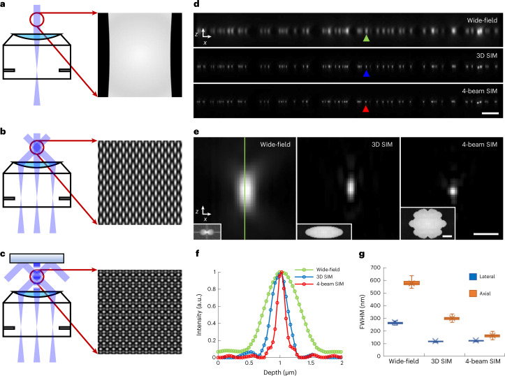
Fig. 1
Improving axial resolution in 3D SIM.
a u2013 c , Schematic representations of beam illumination at objective back focal plane (BFP) and sample planes for wide-field microscopy (single-beam illumination, a ), 3D SIM (three-beam illuminati...
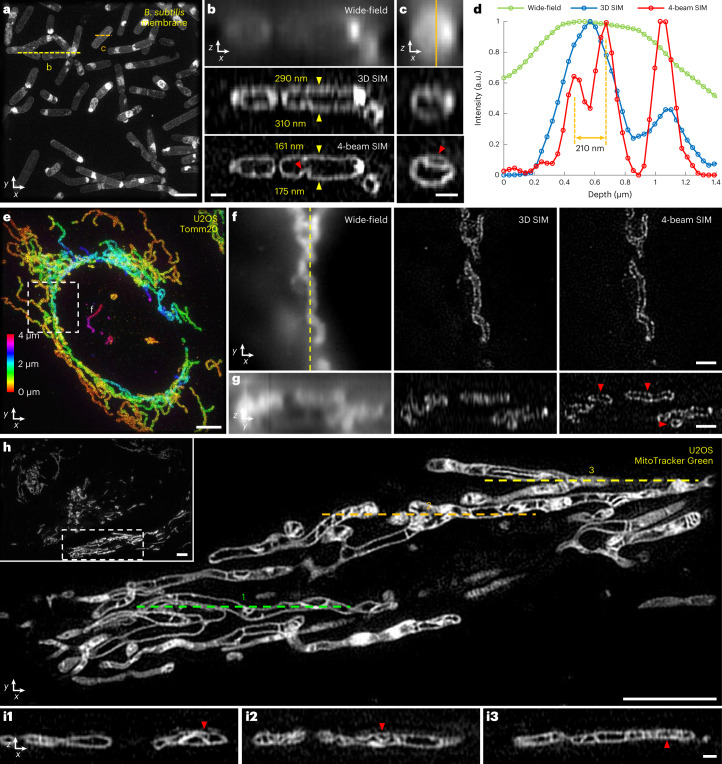
Fig. 2
Four-beam SIM enables near-isotropic imaging of biological samples.
a , Maximum intensity projection of live vegetative B. subtilis stained with CellBrite Fix 488, marking membranes, imaged in four-beam SIM. b , c , Axial views along yellow ( b ) and orange ( c ) dash...
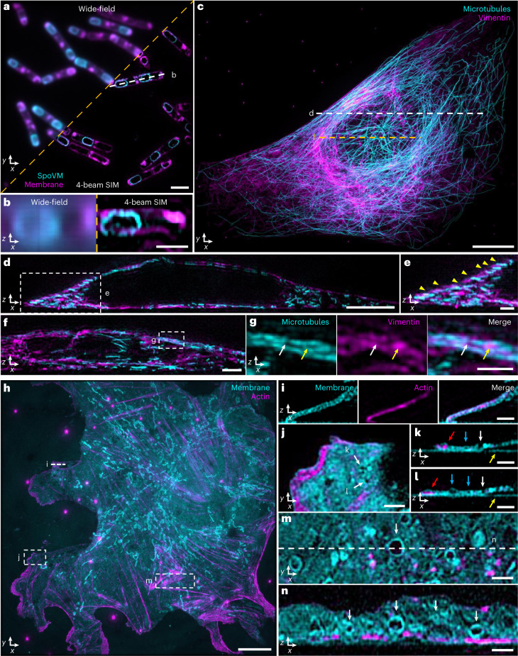
Fig. 3
Near-isotropic imaging in two colors via four-beam SIM.
a , Single lateral plane of live, sporulating B. subtilis with SpoVM-GFP label, marking spores (cyan), and CellBrite Fix 555 label, marking membrane (magenta). b , Axial view (single plane) along whit...
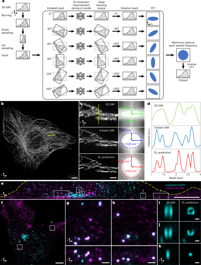
Fig. 4
Deep learning for axial resolution enhancement.
a , Schematic of deep learning process. 3D SIM image volumes are blurred, downsampled and upsampled (each along the lateral x direction) to render isotropic, low-resolution input data (resolution equi...
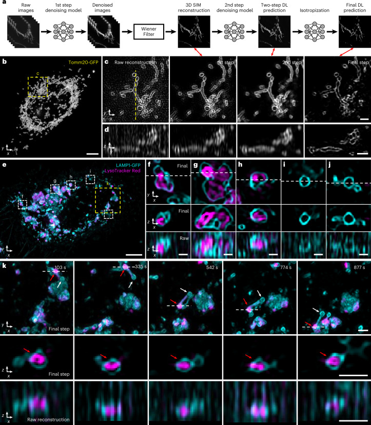
Fig. 5
Denoising and axial resolution enhancement facilitate 4D super-resolution imaging with isotropic resolution.
a , Schematic illustrating workflow for applying deep learning to raw input data. Sets of raw images (5 phases u00d7 3 orientations) are denoised and combined with a generalized Wiener filter; and the...
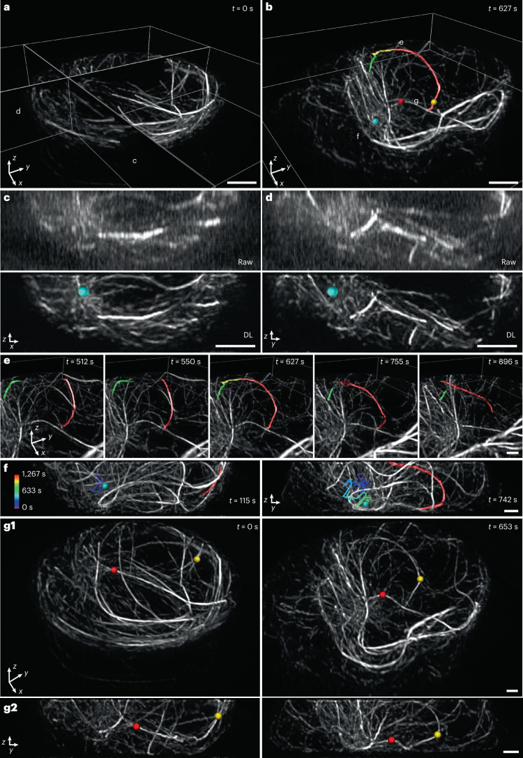
Fig. 6
Denoising and axial resolution enhancement unveil rich microtubule dynamics within a living immune cell.
a , b , Selected volumetric reconstructions of Jurkat T cells expressing EMTB 3u00d7 GFP are shown from 100-timepoint series (volumes recorded every 12.8u2009seconds) in perspective views. In b , the ...
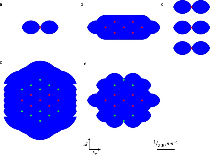
Extended Data Fig. 1
Support of optical transfer functions assuming a silicone oil objective lens.
Axial cross sections through support are shown for a ) wide-field, b ) 3D SIM, c) standing wave, d ) I 5 S, and e ) four-beam, mirror-based SIM systems. Dots indicate illumination spatial frequency co...
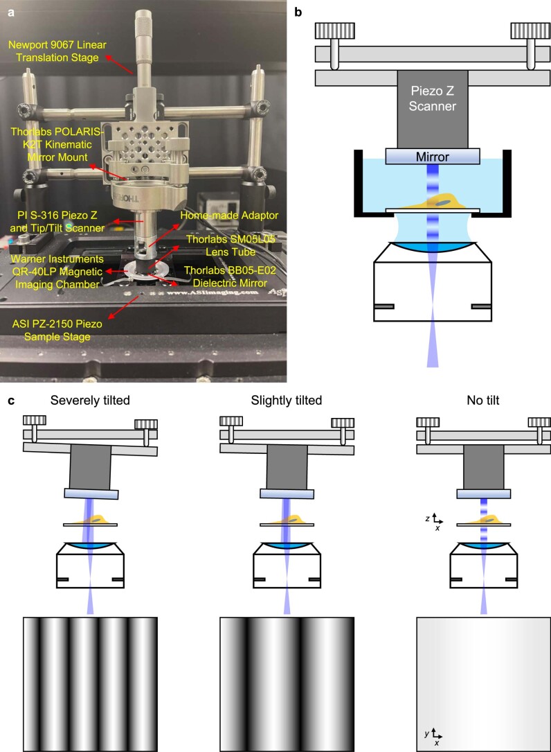
Extended Data Fig. 2
Mounting and aligning reflective mirror for four-beam SIM.
a ) Photograph of mounting scheme, indicating hardware mounts with vendor information. PI: Physik Instrumente. b ) Schematic to accompany a ), showing kinematic mirror mount, Piezo Z scanner, mirror, ...
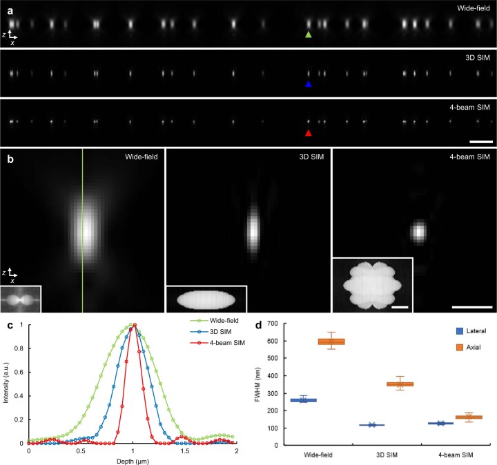
Extended Data Fig. 3
Estimating spatial resolution for 1.27 NA water lens.
a ) x-z cross sectional views of 100u2009nm yellow-green beads, as viewed with wide-field microscopy (top), 3D SIM (middle), and four-beam SIM (bottom). Scale bar: 2u2009u00b5m. b ) Higher magnificati...
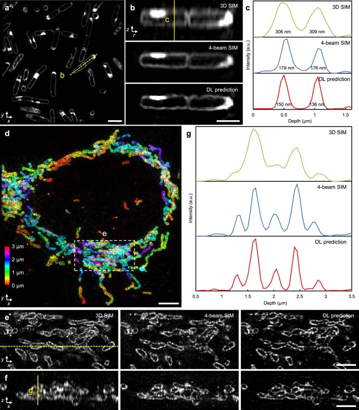
Extended Data Fig. 4
Images of additional samples, comparing deep learning isotropization output to 3D SIM and four-beam SIM.
a ) DL prediction images of live B. subtilis stained for membrane (CellBrite Fix 488). b ) Axial views along dashed yellow line shown in a ), comparing 3D SIM (top), four-beam SIM (middle), and deep l...
Figure images are served from the NIH/NLM PubMed Central Open Access Subset or Europe PMC; copyright remains with the publishers and authors.
💬 Discussion
0 commentsNo comments yet. Be the first to start a discussion!
Leave a Comment