Abstract
AbstractFunctional ultrasound imaging (fUS) is an emerging technique that detects changes of cerebral blood volume triggered by brain activation. Here, we investigate the extent to which fUS faithfully reports local neuronal activation by combining fUS and two-photon microscopy (2PM) in a co-registered single voxel brain volume. Using a machine-learning approach, we compute and validate transfer functions between dendritic calcium signals of specific neurons and vascular signals measured at both microscopic (2PM) and mesoscopic (fUS) levels. We find that transfer functions are robust across a wide range of stimulation paradigms and animals, and reveal a second vascular component of neurovascular coupling upon very strong stimulation. We propose that transfer functions can be considered as reliable quantitative reporters to follow neurovascular coupling dynamics.
🔬 Techniques
🔭 Microscopes
✨ Fluorophores
🧪 Sample Preparation
🏭 Microscope Brands
🧪 Reagent Suppliers
🔴 Lasers
📷 Detectors
🔎 Objectives
🎨 Filters
💻 Software Details
💾 Data Repositories
🏛️ Research Organizations (ROR)
Affiliated research institutions:
📋 Methods
Animal preparation
All animal care and experimentations were performed in accordance with the INSERM Animal Care and Use Committee guidelines (protocol numbers CEEA34.SC.122.12 and CEEA34.SC.123.12). Adult mice ( n = 15, 3–12 months old, 20–35 g, both males and females, housed in 12 h light–dark cycle at 24 °C and 50% humidity, fed ad libitum) were used in this study. Thy1-GCaMP6f (GP5.11) 41 mice were obtained from Jackson laboratory and crossed with M72 - > S50-IRES-hChRVenus mice 42 kindly provided by Thomas Bozza (Department of Neurobiology, Northwestern University, USA). Surgery, anesthesia and the experimental sedation protocol were performed as previously 22 . For craniotomies, mice were initially anesthetized with an intraperitoneal bolus of ketamine–medetomidine (100 and 10 mg kg −1 body mass, respectively). Anesthesia lasted about 2 h, enough to perform the whole surgery. During surgery, mice freely breathed air supplemented with oxygen (final concentration of 40%) and body temperature was maintained at 36 ± 0.5 °C using a rectal probe and a heating pad. The bone over the OBs was carefully drilled while taking care of not applying pressure and avoiding heat with repetitive applications of a cool ACSF solution 43 . A sheet of PMP, either 80 or 125 μm thick) was precisely cut to fit the cranium opening and sealed in place with Tetric Evoflow dental cement (Ivoclar Vivadent AG, Schaan, Liechtenstein). The same dental cement was also used to form a head-cap in which a titanium head-bar was embedded after the bone was treated with a primer, Optibond FL (Kerr Italia S.RL., Salerno, Italia). Antibiotics and anti-inflammatory were administered as in 43 using Baytril 10% (Bayer, Germany) and Dexazone (Virbac, France) respectively. Buprecare (Axience, France) was used to relieve pain. Mice were permitted to recover for at least 2 weeks before the experimental sessions began. Experiments were performed under light sedation: mice were anesthetized for 2 min with 3% isofluorane and then head-fixed while isofluorane was lowered to 2%. A subcutaneous catheter was placed dorsally and medetomidine injected first as a bolus (0.05 mg kg −1 ) and then immediately at a rate of 0.15 mg kg −1 h −1 , which was maintained during the whole experiment. Isofluorane was progressively removed within 40 min. An additional 20 min delay was kept prior to recording. Note that sedation was stable and reliable after 2–3 priming sessions during which the exact same protocol was applied but without recording. During the experiments, breathing was monitored with an 80-μm-tip thermocouple (Omega 5TC-TT-KI-40-1M) connected to a N9212 amplifier (National Instruments, USA) and digitized with a cDAQ-9171 (National Instruments, USA). The thermocouple was placed in front of one of the mouse nostrils and the body temperature was maintained at 36.5 ± 0.5 °C using a rectal probe + heating pad (FHC, Bowdoin, ME). Mice were supplemented with 40% O 2 throughout all experiments.
Show full methods section
Animal preparation
All animal care and experimentations were performed in accordance with the INSERM Animal Care and Use Committee guidelines (protocol numbers CEEA34.SC.122.12 and CEEA34.SC.123.12). Adult mice ( n = 15, 3–12 months old, 20–35 g, both males and females, housed in 12 h light–dark cycle at 24 °C and 50% humidity, fed ad libitum) were used in this study. Thy1-GCaMP6f (GP5.11) 41 mice were obtained from Jackson laboratory and crossed with M72 - > S50-IRES-hChRVenus mice 42 kindly provided by Thomas Bozza (Department of Neurobiology, Northwestern University, USA). Surgery, anesthesia and the experimental sedation protocol were performed as previously 22 . For craniotomies, mice were initially anesthetized with an intraperitoneal bolus of ketamine–medetomidine (100 and 10 mg kg −1 body mass, respectively). Anesthesia lasted about 2 h, enough to perform the whole surgery. During surgery, mice freely breathed air supplemented with oxygen (final concentration of 40%) and body temperature was maintained at 36 ± 0.5 °C using a rectal probe and a heating pad. The bone over the OBs was carefully drilled while taking care of not applying pressure and avoiding heat with repetitive applications of a cool ACSF solution 43 . A sheet of PMP, either 80 or 125 μm thick) was precisely cut to fit the cranium opening and sealed in place with Tetric Evoflow dental cement (Ivoclar Vivadent AG, Schaan, Liechtenstein). The same dental cement was also used to form a head-cap in which a titanium head-bar was embedded after the bone was treated with a primer, Optibond FL (Kerr Italia S.RL., Salerno, Italia). Antibiotics and anti-inflammatory were administered as in 43 using Baytril 10% (Bayer, Germany) and Dexazone (Virbac, France) respectively. Buprecare (Axience, France) was used to relieve pain. Mice were permitted to recover for at least 2 weeks before the experimental sessions began. Experiments were performed under light sedation: mice were anesthetized for 2 min with 3% isofluorane and then head-fixed while isofluorane was lowered to 2%. A subcutaneous catheter was placed dorsally and medetomidine injected first as a bolus (0.05 mg kg −1 ) and then immediately at a rate of 0.15 mg kg −1 h −1 , which was maintained during the whole experiment. Isofluorane was progressively removed within 40 min. An additional 20 min delay was kept prior to recording. Note that sedation was stable and reliable after 2–3 priming sessions during which the exact same protocol was applied but without recording. During the experiments, breathing was monitored with an 80-μm-tip thermocouple (Omega 5TC-TT-KI-40-1M) connected to a N9212 amplifier (National Instruments, USA) and digitized with a cDAQ-9171 (National Instruments, USA). The thermocouple was placed in front of one of the mouse nostrils and the body temperature was maintained at 36.5 ± 0.5 °C using a rectal probe + heating pad (FHC, Bowdoin, ME). Mice were supplemented with 40% O 2 throughout all experiments.
Odor stimulation
All the experiments were conducted following the same stimulation protocol and materials, so no blinding was performed. Odors were delivered through a home built olfactometer. Odor and exhaust lines were equilibrated for pressure at the start of each experiment and the odor concentration and temporal profile was calibrated at the tubing end before every experiment, using a photo-ionization detector (miniPID 200B, Aurora Scientific, Aurora, Canada). The concentration reached 90% of steady state within ∼50 ms and returned to baseline within the same range. The final odor concentration values were calculated after considering the dilution from the supplemental O 2 line that did not pass through the olfactometer. To compare the responses to different odor durations or concentrations, the stimulations were randomly interleaved, discarding anesthesia-related changes. All microscopic (2PM) and mesoscopic (fUS) acquisitions lasted 30 s, with the exception of strong stimulations (6% ET, 5 s), for which 60 s acquisitions were used to allow complete recovery to baseline. All the traces reported in the figures represent the average of at least three odor applications, with the exception of Fig. 3a , top panel (two traces). Single sniff (120 ms) were usually averaged over 8–12 applications because of the low signal-to-noise ratio, in particular at 1% ET. The odor delivery was finely time-locked with the inhalation period, detected with the nasal thermocouple. fUS data acquisition and post processing fUS imaging was performed as follows 22 . In brief, a linear ultrasound probe (128 elements, 15 MHz central frequency, Vermon, Tours, France), connected to the ultrasound scanner (AixplorerTM, Supersonic Imagine, Aix-en-Provence, France), was placed 3 mm above the window. Custom transmit/receive ultrasound sequences were written in Matlab (Mathworks, USA). The backscattered echoes of ultrasound plane waves were collected and beam formed to produce OB echographic images, in the coronal plane. To increase the SNR of each echographic image taken at 500 Hz, the echographic images were compounded by transmitting several tilted plane waves and adding their backscattered echoes. The compounded sequence resulted in enhanced echographic images, thereby increasing the sensitivity of the Doppler measurement without aliasing in the mouse brain. In this study, the ultrasound sequence consisted of transmitting eleven different tilted plane waves (from −10° to 10° in 2° increments) with a 5500 Hz pulse repetition frequency (500 Hz final frame rate). Tissue signals were removed from backscattered waves using singular value decomposition and elimination of the largest eingenvalues. The Power Doppler was further filtered with a Butterworth filter (fifth order, 10–30 Hz band-pass). Each voxel signal was obtained by the incoherent temporal average of the blood signal. Voxel size at the focal plane was: 100 × 110 μm ( x and z direction) and 200 μm ( y direction,i.e., slice thickness). fUS analysis All analyses were performed with custom made software developed in Matlab 2018a (Mathworks, USA). Beam-formed data resulted in 500 Hz frame rate time series. GLM analysis of fUS data was performed with SPM12. fUS recordings were single voxel under-sampled at 20 Hz using a cubic interpolation (‘ interp1 ’ function, ‘ pchip ’ option, Matlab). Each frame was then converted to a NIfTI file. The absence of movement was previously assessed using a custom made Matlab script. No realignment or spatial smoothing was performed with SPM. Regressors used in GLM analyses were the RBC velocities recorded in the same mice. We applied a statistical threshold of p < 0.01 + FEW correction, in response to each stimulation condition. 2PM acquisition and data analysis 2PM imaging was performed using an ultra-flexible microscope 44 and data were collected and analyzed using a custom software. Eighty femtoseconds laser pulses were delivered by a Ti:Sapphire laser at 80 MHz (MaiTai HP DeepSee, MKS-Spectra Physics, Santa Clara, California). An acousto optic modulator (MT110B50-A1.5-IR-Hk, AA Optoelectronic, Orsay, France) was used to modulate the laser power. Laser pulses were scanned on the sample with galvanometric mirrors (6215H Cambridge Technology, Bedford, Massachusetts). The excitation light was forwarded through a dichroic mirror (cut-off wavelength, 775 nm FF775-DiO1 Semrock) and focused on the sample with a 20 × 1.0 NA objective (XLUMPLFLN20XW Olympus, Tokyo, Japan). GCaMP6f and Texas Red were excited at 920 nm. The collected emission was separated in two channels with a dichroic mirror (cut-off wavelength, 560 nm FF560-DiO1 Semrock). The signal was filtered with a 525 nm band pass filter (FF03-525/50 Semrock) in the « green channel » and a 620 nm band pass filter (620 nm FF01-624/40 Semrock) in « the red channel ». In both channels, GaAsP PMTs (H10770PA-40; Hamamatsu Photonics, Japan) were used to collect light, and laser reflections were blocked with short pass filters (FF01-750/SP-25 Semrock). PMT signals were amplified, integrated with a custom-built electronic circuit and sampled with a National Instruments acquisition card (PCI 6115). Vessels were labeled with Texas Red dextran (70 kDa, Molecular Probes, ThermoFisher, Waltham, Massachusetts), administered intravenously by retro-orbital injections. Following mapping of the ET activated region in frame scan mode and selection of the most sensitive glomerulus to the odor, broken linescan recordings were performed to record both RBC velocity and Ca 2+ signals in the neuropil, as previously described 7 . Linescan acquisitions (1.5–3 ms per line) were repeated during the different stimulation protocols, with 3 min between each trial. Ca 2+ data were interpolated (10 ms cubic interpolation, ‘ interp1 ’ function, ‘ pchip ’ option, Matlab), turned into ΔCa 2+ traces by subtracting the average value of the last 5 s of baseline. RBC velocities were extracted and analyzed using a custom software 22 . RBC velocity data were interpolated (200 ms, cubic interpolation, ‘ interp1 ’ function, ‘ pchip ’ option, Matlab), turned into ΔRBC/RBC traces by subtracting the average value of the last 5 s of baseline and then dividing by it. A median filter of three time points was applied to some traces to attenuate overestimated RBC velocity values.
Co-registration of fUS and two-photon imaging
To ensure that we image the same brain volume with fUS and 2PM, we attached the ultrasonic probe to microscope objective with a custom printed ABS holder (Makerbot 2×, USA). A 50-μm glass bead (Marteau & Lemarié, Sorbiers, France), embedded in 2.5% agar, was first localized with 2PM and then detected with the ultrasonic probe, translated to a position such that the bead fUS signal maxima in x , y , and z were centered in a given voxel (Fig. 4a ). The fUS and 2PM imaging systems could then be displaced back and forth to the same co-registered location with a micrometric resolution. Note that in our experimental conditions, two factors may have influenced the speed of sound and thus cause approximation along the z axis: the temperature of the media (brain tissue) and the thickness of the PMP cranial window, both of them creating a Δz approximation ≤ 25 μm, for a mean speed of sound of ∼1500 m s −1 .
TF computation
The transfer function captures the dynamic link between neuronal responses and micro/mesoscopic vascular responses. Using Ca 2+ and RBC velocity data collected with 2PM and fUS CBV data within the co-registered brain volume, we built TFs across the different imaging modalities. We used a fitting approach with a single-gamma distribution function, as there was no undershoot in flow in our data. We added a time-shift parameter with the heaviside unit step function, resulting in a total of four parameters for the optimization problem. These parameters capture the slope, the decay, the amplitude and time-shift, respectively, but they are not independent from each other: the optimization problem presents multiple minima configurations, a condition that is not favorable for quasi-Newtonian optimization algorithms. All analyses were performed with a custom-written software in Matlab 2018a. The four-parameters function, documentclass[12pt]{minimal} usepackage{amsmath} usepackage{wasysym} usepackage{amsfonts} usepackage{amssymb} usepackage{amsbsy} usepackage{mathrsfs} usepackage{upgreek} setlength{oddsidemargin}{-69pt} begin{document}$${mathrm{TF}}left( t right) = {mathrm{H}}( t - p_3 ) p_4 left( {frac{{( t - p_3 )^{p_1 - 1} p_2 ^ {p_1} {mathrm{e}}^{ - p_2left( {t - p_3} right)}}}{{Gamma left( {p_1} right)}}} right)$$end{document} TF t = H ( t − p 3 ) p 4 ( t − p 3 ) p 1 − 1 p 2 p 1 e − p 2 t − p 3 Γ p 1 , was optimized by minimizing the sum of the square residuals, using simulated annealing, a machine-learning algorithm (‘ simulannealbnd ’ function, Matlab). Note that this is a nondeterministic algorithm: the same set of initial values can bring to different sets of optimized values for the parameters, unless the initial set represent a stable minimum for the optimization function. Note that it was not necessary to modify the Matlab default initial temperature (100) and temperature function (‘ temperatureexp ’ function, Matlab). Lower and upper boundaries were set to 10 −3 and 10, respectively, for all parameters. Upper bounds were occasionally increased up to 20 during some optimizations. For Ca 2+ to RBC velocity optimization the presence of the time shift granted a better fit of the onset phase of the responses. For Ca 2+ to fUS optimization, we used a 0–0.5 s time shift. Transfer functions were computed between two time series ( From and To ). Both were cut between 5 and 27 s (for 30 s acquisitions) and between 5 and 59 s (for 60 s acquisitions). From signals were Ca 2+ responses and were interpolated at 50 ms (cubic interpolation, ‘ interp1 ’ function, ‘ pchip ’ option, Matlab), as Ca 2+ data can be noisy. To signals were either RBC velocity responses, or 1 and 6 voxels Power Doppler responses. The residual sum was computed as the difference between the To signal and the convolution of the From signal and the TF, down sampled to match To . Simulated annealing being a nondeterministic algorithm, the initial values of the parameters are crucial for the outcome and the same set of initial values can bring to different outcomes at each optimization run. We used an iterative process for which we started with an initial set of values (the ones of the first gamma-component of the standard HRF (6; 1; 0.001; 1) with the time-shift initially set to zero (0.001 for computational requirements), and run the optimization process multiple times (50–100 times). We then scored the final sets of values based on the prediction quality and we took the set with the best prediction, provided its corresponding function started at the origin of the axes and was derivable at least twice (after the time-shift time). This set was then used as an initial set for another batch of multiple runs, and so on, until the algorithm did not improve anymore the prediction made by the set of initial values in a significant manner. Usually this took no more than three iterations (see Supplementary Fig. 1 ). The best set of parameter values determined the TF optimized for a given mouse in response to 1% ET, 5 s. We computed the best parameters set for all the 15 recorded mice and checked each TF to find the best one across all mice by means of a leave-one-out cross-validation. In detail, each TF, optimized in a given mouse dataset, was then used to predict the vascular responses of the rest of dataset made other mice recordings. The best TFs, finally called µTF or M TF, were chosen being the best performing on its dataset and on dataset from other mice, on the basis of the highest average Pearson coefficient and smallest coefficient of variability, the first preferred when the two conditions were not met by any mouse. Numerical values of the optimized TF parameters are provided in Table 1 . Table 1 Parameters of the different TFs computed in this study. From > To p 1 p 2 p 3 p 4 (amplitude) Single-gamma HRF 6 1 0 1 Ca 2+ to RBC velocity (ET 1%, 5 s) 1.3 0.5 0.27 0.19 Ca 2+ to Single voxel fUS* (ET 1%, 5 s) 1.99 1.27 0.11 0.045 Source data are provided as a Source Data file. *0 < Time shift (P3) < 0.5. Analysis of data from Rungta et al. Vascular responses are those described as juxta-synaptic capillary in Fig. 7 of the original paper 5 . TF was computed as before, except for the fact that time series were only 15 s long. Data were collected in four OB glomeruli from three different mice 5 . Analysis of data from Winder et al. Data from the original paper 27 are available on the following link: https://psu.app.box.com/v/Winder2017-Code-Data . We used the data (gamma-band LFP and IOS reflection changes in response to contralateral whisker stimulations) from the 12 mice (*_EVENTDATA_ files). We averaged every trace for both gamma-band LFP and IOS reflection changes. Data were changed into relative values and then averaged for each mouse. TF was computed as before 27 .
Prediction computation
Micro and mesoscopic vascular predictions were computed by convoluting the Ca 2+ responses or the step functions with the correspondent TFs. An optimization of the amplitude of the responses was performed to best match predictions over experimental data. We optimized a scaling factor with a classical derivative-free method (‘ fminsearch ’ function, Matlab) using the residuals between the prediction and vascular responses from 2 to 8 s after the odor application onset as a cost function. The final prediction was then multiplied by the optimized scaling factor. Note, this post processing does not affect the Pearson coefficient we used for all the quantifications of the study. Custom made scripts to compute the TFs A simple graphical user interface version of our scripts is available on GitLab ( https://gitlab.com/AliK_A/buildtf ), as well as some data examples in order to give the opportunity to the reader to compute the TFs.
Statistical tests
All statistical analyses are reported in the manuscript, with p values. A confidence level of 5% was chosen, a priori, as threshold for significant difference between samples, however higher confidence levels are reported in some figures, with graphical indicators of p values. Reporting summary Further information on research design is available in the Nature Research Reporting Summary linked to this article.
Supplementary information Supplementary Information Peer Review File Reporting Summary
📊 Figures
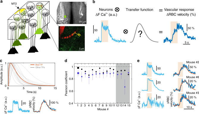
Fig. 1
The transfer function between neuronal and vascular responses within a single glomerulus: computation and robustness across mice.
a Left, schematics of the dorsal olfactory bulb (OB) of a mouse expressing YFP and GCaMP6f under the control of M72 and Thy1 promoters, respectively. Depending on the odor concentration, ethyl tiglate...
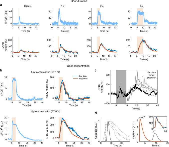
Fig. 2
Robustness of TFs with respect to stimulation duration and intensity.
a Ca 2+ (top) and RBC velocity (bottom) responses to single sniff (120u2009ms), 1u2009s, 2u2009s, and 5u2009s odor stimulations. Using the standard u03bcTF (optimized with ET 1%, 5u2009s), vascular re...
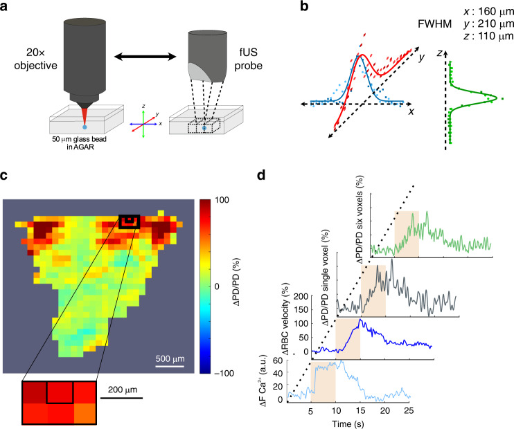
Fig. 3
Co-registration of fUS (single voxel) and two-photon imaging.
a Schematics of the two imaging systems. The ultrasonic probe is attached to the u00d720 microscope objective by means of a 3D-printed holding system. A 50-u03bcm glass bead, embedded in agar, is firs...
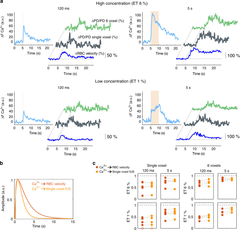
Fig. 4
Co-registration of microscopic and mesoscopic vascular responses to odor.
a Microscopic responses were acquired in a glomerulus located in the center of a fUS voxel. The four panels illustrate Ca 2+ , RBC velocity, and the three types of fUS responses (from the specific co-...
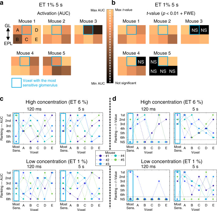
Fig. 5
Spatial resolution of fUS responses.
a Quantification of fUS responses (area under the curve, ET 1%, 5u2009s) in the voxel containing the most sensitive glomerulus (outlined with a blue frame) and the five neighboring voxels (Au2013E, n ...
Figure images are served from the NIH/NLM PubMed Central Open Access Subset or Europe PMC; copyright remains with the publishers and authors.
💬 Discussion
0 commentsNo comments yet. Be the first to start a discussion!
Leave a Comment