Abstract
Abstract By virtue of the combined merits of flow cytometry and fluorescence microscopy, imaging flow cytometry (IFC) has become an established tool for cell analysis in diverse biomedical fields such as cancer biology, microbiology, immunology, hematology, and stem cell biology. However, the performance and utility of IFC are severely limited by the fundamental trade-off between throughput, sensitivity, and spatial resolution. Here we present an optomechanical imaging method that overcomes the trade-off by virtually freezing the motion of flowing cells on the image sensor to effectively achieve 1000 times longer exposure time for microscopy-grade fluorescence image acquisition. Consequently, it enables high-throughput IFC of single cells at >10,000 cells s −1 without sacrificing sensitivity and spatial resolution. The availability of numerous information-rich fluorescence cell images allows high-dimensional statistical analysis and accurate classification with deep learning, as evidenced by our demonstration of unique applications in hematology and microbiology.
🔬 Techniques
🔭 Microscopes
🧬 Organisms
💻 Software
✨ Fluorophores
🧪 Sample Preparation
🔬 Cell Lines
🏭 Microscope Brands
🧪 Reagent Suppliers
🔴 Lasers
📷 Detectors
🎨 Filters
💻 Software Details
💾 Data Repositories
🏛️ Research Organizations (ROR)
Affiliated research institutions:
📋 Methods
Optical design
The optical system of the VIFFI flow cytometer was designed so that it has both subcellular spatial resolution and high-throughput comparable to conventional (non-imaging) flow cytometers. On the basis of this concept, we firstly chose an objective lens (Olympus UPLSAPO20x, NA = 0.75) and a tube lens (Olympus U-TLU, f = 180 mm) to obtain subcellular resolution. Subsequently, we determined the magnification of the relay lens systems M and M −1 and the number of facets of the polygon scanner N by considering the following constraints: (i) The image frames should be concatenated so that whole images of all flowing cells fall in one of the continuous frames (Fig. 1c ); (ii) The fluorescence beam size in the polygon scanner’s facet should be smaller than the facet size (Supplementary Fig. 2a ). In addition, we considered specifications of the sCMOS camera and polygon scanner (Lincoln Laser RTA-B) such as the frame period T s = 0.8 ms (frame rate: 1250 fps) with the region of interest of 2560 × 88 pixels, sensor size in the direction corresponding to the cell flow L x = 16.6 mm, and inner diameter of the polygon mirror of the scanner d p = 70 mm. The above constraints are expressed by the following equations: 1 documentclass[12pt]{minimal} usepackage{amsmath} usepackage{wasysym} usepackage{amsfonts} usepackage{amssymb} usepackage{amsbsy} usepackage{mathrsfs} usepackage{upgreek} setlength{oddsidemargin}{-69pt} begin{document}$$4f_{mathrm{o}}Mleft{ {frac{{2{uppi}}}{N} + sin ^{ - 1}left[ {left( { - frac{{d_{mathrm{o}}M}}{{d_{mathrm{p}}}} + sin alpha } right)cos frac{{uppi }}{N}} right] - sin ^{ - 1}left[ {left( {frac{{d_{mathrm{o}}M}}{{d_{mathrm{p}}}} + sin alpha } right)cos frac{{uppi }}{N}} right]} right}, > , 0,$$end{document} 4 f o M 2 π N + sin − 1 − d o M d p + sin α cos π N − sin − 1 d o M d p + sin α cos π N > 0 , 2 documentclass[12pt]{minimal} usepackage{amsmath} usepackage{wasysym} usepackage{amsfonts} usepackage{amssymb} usepackage{amsbsy} usepackage{mathrsfs} usepackage{upgreek} setlength{oddsidemargin}{-69pt} begin{document}$$frac{{vT_{mathrm{s}}N}}{{4{uppi}f_{mathrm{o}}}}, < , M, < , frac{{L_xN}}{{4{uppi}f_{mathrm{t}}}},$$end{document} v T s N 4 π f o < M < L x N 4 π f t , where f o , α , d o , v , f t denote the focal length of the objective lens (9 mm), the nominal incidence angle of the fluorescence to the polygon scanner (45 degrees), the back-aperture diameter of the objective lens (13.5 mm), the flow speed of the cells (1 m s −1 ), and the focal length of the tube lens (180 mm), respectively. The left hand side of Eq. ( 1 ) corresponds to the maximum scan range of the polygon scanner on the object and thus represents the maximum exposure duration. A plot of the maximum scan range under the above constraints is shown in Supplementary Fig. 2b . The scan range divided by the flow speed represents the upper limit on the exposure time. The figure shows that a lower magnification value is beneficial for obtaining a longer exposure time. As a trade-off, in practice, a relay lens system with a lower magnification tends to have larger aberration, which degrades the imaging quality. Therefore, we chose M = 0.2 and N = 28 so that the aberration that occurs in the relay lens systems does not significantly degrade the imaging quality (see below for the detailed design of the relay lens systems) while significant improvement of the imaging sensitivity is obtained. Excitation beam scan The excitation beam scan is an essential part of the VIFFI flow cytometer to enable its exceptionally long exposure time for fast-flowing cells. A schematic of the beam scan is shown in Supplementary Fig. 4a . A focused excitation beam with a diameter of 26 μm in the cell flow direction is scanned in the direction opposite to the cell flow at 2.54 m s −1 (a speed relative to flowing cells), limiting the local exposure time to 10 μs. Since the FOV of the camera in the object plane moves together with the cell flow during the exposure time, the scan range (525 μm) is shorter than the FOV in the flow direction (830 μm), which significantly reduces the off-axis aberration components such as image distortion and field curvature. In particular, the image distortion that occurs between the object and the polygon scanner causes position-dependent errors of the motion cancellation effect of the polygon scanner and hence residual motion of the cell images, which limits extension of the exposure time. We experimentally determined the speed of the residual motion using obtained images of fluorescent particles. The results shown in Supplementary Fig. 4b indicate that the speed range of the residual motion is ±1.5% with the beam scan while it is at least ±6% without the beam scan. Assuming a typical speed fluctuation of flowing cells in a microfluidic channel of 1.5%, the factors for the extension of exposure time per pixel in the VIFFI flow cytometer are (0.015 + 0.015) −1 ≈ 33 with the beam scan and (0.06 + 0.015) − 1 ≈ 13 without the beam scan. Moreover, due to the confined excitation beam width in the flow direction (~3% of the FOV of the sCMOS camera), the excitation efficiency improves by a factor of 1/0.03 ≈ 33 under a certain excitation beam power whereas the total exposure time of the camera is extended by the same factor. As a result, the improvement factor of the imaging sensitivity of the VIFFI flow cytometer is 33 × 33 ≈ 1000 with the beam scan while it is limited to ~13 without the beam scan.
Show full methods section
Optical design
The optical system of the VIFFI flow cytometer was designed so that it has both subcellular spatial resolution and high-throughput comparable to conventional (non-imaging) flow cytometers. On the basis of this concept, we firstly chose an objective lens (Olympus UPLSAPO20x, NA = 0.75) and a tube lens (Olympus U-TLU, f = 180 mm) to obtain subcellular resolution. Subsequently, we determined the magnification of the relay lens systems M and M −1 and the number of facets of the polygon scanner N by considering the following constraints: (i) The image frames should be concatenated so that whole images of all flowing cells fall in one of the continuous frames (Fig. 1c ); (ii) The fluorescence beam size in the polygon scanner’s facet should be smaller than the facet size (Supplementary Fig. 2a ). In addition, we considered specifications of the sCMOS camera and polygon scanner (Lincoln Laser RTA-B) such as the frame period T s = 0.8 ms (frame rate: 1250 fps) with the region of interest of 2560 × 88 pixels, sensor size in the direction corresponding to the cell flow L x = 16.6 mm, and inner diameter of the polygon mirror of the scanner d p = 70 mm. The above constraints are expressed by the following equations: 1 documentclass[12pt]{minimal} usepackage{amsmath} usepackage{wasysym} usepackage{amsfonts} usepackage{amssymb} usepackage{amsbsy} usepackage{mathrsfs} usepackage{upgreek} setlength{oddsidemargin}{-69pt} begin{document}$$4f_{mathrm{o}}Mleft{ {frac{{2{uppi}}}{N} + sin ^{ - 1}left[ {left( { - frac{{d_{mathrm{o}}M}}{{d_{mathrm{p}}}} + sin alpha } right)cos frac{{uppi }}{N}} right] - sin ^{ - 1}left[ {left( {frac{{d_{mathrm{o}}M}}{{d_{mathrm{p}}}} + sin alpha } right)cos frac{{uppi }}{N}} right]} right}, > , 0,$$end{document} 4 f o M 2 π N + sin − 1 − d o M d p + sin α cos π N − sin − 1 d o M d p + sin α cos π N > 0 , 2 documentclass[12pt]{minimal} usepackage{amsmath} usepackage{wasysym} usepackage{amsfonts} usepackage{amssymb} usepackage{amsbsy} usepackage{mathrsfs} usepackage{upgreek} setlength{oddsidemargin}{-69pt} begin{document}$$frac{{vT_{mathrm{s}}N}}{{4{uppi}f_{mathrm{o}}}}, < , M, < , frac{{L_xN}}{{4{uppi}f_{mathrm{t}}}},$$end{document} v T s N 4 π f o < M < L x N 4 π f t , where f o , α , d o , v , f t denote the focal length of the objective lens (9 mm), the nominal incidence angle of the fluorescence to the polygon scanner (45 degrees), the back-aperture diameter of the objective lens (13.5 mm), the flow speed of the cells (1 m s −1 ), and the focal length of the tube lens (180 mm), respectively. The left hand side of Eq. ( 1 ) corresponds to the maximum scan range of the polygon scanner on the object and thus represents the maximum exposure duration. A plot of the maximum scan range under the above constraints is shown in Supplementary Fig. 2b . The scan range divided by the flow speed represents the upper limit on the exposure time. The figure shows that a lower magnification value is beneficial for obtaining a longer exposure time. As a trade-off, in practice, a relay lens system with a lower magnification tends to have larger aberration, which degrades the imaging quality. Therefore, we chose M = 0.2 and N = 28 so that the aberration that occurs in the relay lens systems does not significantly degrade the imaging quality (see below for the detailed design of the relay lens systems) while significant improvement of the imaging sensitivity is obtained. Excitation beam scan The excitation beam scan is an essential part of the VIFFI flow cytometer to enable its exceptionally long exposure time for fast-flowing cells. A schematic of the beam scan is shown in Supplementary Fig. 4a . A focused excitation beam with a diameter of 26 μm in the cell flow direction is scanned in the direction opposite to the cell flow at 2.54 m s −1 (a speed relative to flowing cells), limiting the local exposure time to 10 μs. Since the FOV of the camera in the object plane moves together with the cell flow during the exposure time, the scan range (525 μm) is shorter than the FOV in the flow direction (830 μm), which significantly reduces the off-axis aberration components such as image distortion and field curvature. In particular, the image distortion that occurs between the object and the polygon scanner causes position-dependent errors of the motion cancellation effect of the polygon scanner and hence residual motion of the cell images, which limits extension of the exposure time. We experimentally determined the speed of the residual motion using obtained images of fluorescent particles. The results shown in Supplementary Fig. 4b indicate that the speed range of the residual motion is ±1.5% with the beam scan while it is at least ±6% without the beam scan. Assuming a typical speed fluctuation of flowing cells in a microfluidic channel of 1.5%, the factors for the extension of exposure time per pixel in the VIFFI flow cytometer are (0.015 + 0.015) −1 ≈ 33 with the beam scan and (0.06 + 0.015) − 1 ≈ 13 without the beam scan. Moreover, due to the confined excitation beam width in the flow direction (~3% of the FOV of the sCMOS camera), the excitation efficiency improves by a factor of 1/0.03 ≈ 33 under a certain excitation beam power whereas the total exposure time of the camera is extended by the same factor. As a result, the improvement factor of the imaging sensitivity of the VIFFI flow cytometer is 33 × 33 ≈ 1000 with the beam scan while it is limited to ~13 without the beam scan.
Data acquisition sequence
A schematic of the data acquisition sequence is shown in Supplementary Fig. 5 . A trigger signal from a photodetector that indicates the polygon scanner’s angle is used to generate external trigger signals for the camera’s start of exposure and the waveform generator’s signal output. Then, the excitation beam is scanned for ~320 μs during the camera’s exposure time (~340 μs), which is set shorter than the upper limit determined by the design of the imaging optical system (420 μs). The camera outputs image data right after its exposure time. We set the total period of the image acquisition procedure to be slightly less than the polygon scanner’s scan period (800 μs) by adjusting the number of pixel lines in the y direction in the object plane so that every external trigger signal successfully triggers the camera’s exposure start.
Relay lens systems
We designed the relay lens systems using OpticStudio (Zemax, LLC). Considering cost effectiveness, our design assumed only off-the-shelf achromatic lenses from major optics companies. Also, we assumed four achromatic doublets for constituting a single relay lens system rather than two to reduce the total aberration. We created a macro that automatically evaluates the total aberration of ~10,000 relay lens systems, each of which has a different combination of the four achromatic doublets with the designated magnification (0.2) and with an optimized configuration found by the optimization function of OpticStudio. Thus, we found that a relay lens system shown in Supplementary Fig. 6a has diffraction-limited imaging performance. We employed this system to both of the relay lens systems in the setup of the VIFFI flow cytometer. We evaluated optical transfer functions (OTFs) of the whole relay system that consists of the two relay lens systems and a polygon scanner using a combined optical model shown in Supplementary Fig. 6b . The OTFs were calculated at different positions in the image plane indicated in the upper part of Supplementary Fig. 6c , considering the dynamic localized illumination of the excitation beam during the rotation of the polygon scanner. As shown in Supplementary Fig. 6c , we confirmed that the relay system does not suffer from significant image degradation over the entire FOV.
Constructed optical setup
A complete schematic of the VIFFI flow cytometer is shown in Supplementary Fig. 1 . The optical system consists of a light-sheet optical excitation system, an imaging optical system, and an angle detection system for a polygon scanner. In the light-sheet optical excitation system, excitation beams with the desired spatiotemporal profiles in the object plane are created. Two excitation beams from laser sources [Nichia NDS4216 ( λ = 488 nm), MPB Communications 2RU-VFL-P-5000-560-B1R ( λ = 560 nm)] are scanned by a beam scanner (acousto-optic deflector, ISOMET OAD948) and are focused on a microfluidic channel through cylindrical lenses ( f = 80 mm in the x direction and f = 18 mm in the z direction). The designed Gaussian beam diameters (e −2 intensity) on the object plane are 26 μm × 5.2 μm and 23 μm × 6.4 μm ( x × z , see Supplementary Fig. 1 for the coordinates) for the beams of 488 nm and 560 nm, respectively. Since the beam scanner’s deflection angle for a certain frequency of the driving signal is proportional to the wavelength of the incident beam, the scan range for the 488-nm beam, which has the shorter scan range, is set so that it covers the entire FOV. Therefore, the effective exposure time of the 560-nm excitation beam is slightly shorter (488/560 = 86%) than that of the 488-nm excitation beam. In the imaging system, fluorescence images of flowing cells are captured by a sCMOS camera (PCO edge 5.5). Fluorescence signals from the flowing cells are relayed by two relay lens systems with magnifications of 0.2 and 5, respectively, such that images of the cells are formed on the sCMOS camera through a tube lens. The magnification of the imaging system is set to be 20×. A polygon scanner (Lincoln Laser RTA-B) is placed in a conjugate plane of the exit pupil of the objective lens (Olympus UPLSAPO20x, NA = 0.75) that is created between the two relay lens systems. The fluorescence is split into shorter and longer wavelength components by a dichroic mirror (Semrock FF580-FDi01, edge wavelength: 580 nm), each of which forms an image on the sCMOS camera at a different position. The orientation of the sCMOS camera in the optical setup is set by taking its data readout sequence into consideration. Since the sCMOS camera reads out the pixel data line-by-line, the frame rate does not depend on the region of interest in the line direction. Therefore, to operate the camera at the maximum pixel data rate, we set the camera so that the flow direction coincides with the line direction of the camera. In the angle detection system, a timing trigger for synchronized operation of the polygon scanner, beam scanner, and sCMOS camera is generated. A laser beam that reflects at the polygon scanner is focused on a pinhole aperture and is detected by a photodetector. The output voltage signal of the photodetector is used as the timing trigger and then sent to the external trigger input of a trigger generator (Teledyne LeCroy Wavestation 2052). Trigger signals generated by the trigger generator are sent to the external trigger input of the sCMOS camera and the Waveform generator (RIGOL DG 4202) so that they start exposure and generation of a driving signal for the beam scan. Depending on the application, different configurations can be employed. For the experiments in Fig. 3c, d and Supplementary Fig. 7 , we used a 405-nm excitation laser (Oxxius LBX-405-300-CSB-PP) for obtaining images of C. reinhardtii and PC-9 cells. For the experiments in Fig. 3a and Supplementary Fig. 9 , we used a 488-nm excitation laser (Coherent Genesis CX 488 STM) for FISH imaging and the evaluation of the imaging sensitivity, respectively, where the laser beam illuminates the microchannel through an objective lens (Leica, 20×, NA = 0.75) with carefully designed Gaussian beam diameters (e −2 intensity) in the object plane of 31 μm × 62 μm ( x × y , see Supplementary Fig. 1 for the coordinates). We used the same laser for imaging of S. cerevisiae cells (Fig. 3b ) in the standard illumination configuration shown above.
Digital image processing and deep learning
A schematic of our digital image processing is shown in Supplementary Fig. 10 . From a raw image frame obtained by image acquisition software (PCO Camware 4.04), we extracted the region of the image of each color channel. Then, we created a binary mask image for each color channel using standard image segmentation methods. Subsequently, morphological features were calculated from masked or non-masked images of each channel. For murine white blood cells, we calculated the cell nucleus area and enclosing box area (the smallest rectangular box area within which the nucleus lies). For E. gracilis cells, we obtained the number of lipid droplets by counting local maximum points in the images. In order to count lipid droplets, we first set the approximate lipid droplet size and intensity threshold. After that, we used the approximate lipid droplet size to find the areas with the maximum and minimum intensities. Then, we picked the maximum-intensity areas whose intensity differences with surrounding minimum-intensity areas were larger than the threshold and created a Boolean map, which showed the positions of the lipid droplets. In addition, we used a CNN called VGG-16, which is a well-known CNN model, to differentiate between different cell types in our experiments. We made changes to the input layer of the original VGG-16 model in order to make it applicable to our image data. As shown in Supplementary Fig. 18 , the VGG-16 model consists of five convolution segments and a fully connected classifier. Each convolution segment is made of a few convolution layers that extract the features of the image data, and one max pooling layer at the end to reduce the data volume. At the fully connected classifier, 4096 features extracted by the convolution segments were converted into one dimension that provided the classification results. For example, if the input data is a 224 × 224 RGB image, which can be presented as a 224 × 224 × 3 matrix, the first convolutional layer in the first segment (conv1_1) transforms this image into a 224 × 224 × 64 volume. As the image goes through the network, this volume becomes smaller in width and height, but larger in depth. The pooling layer in the fifth segment (pool_5) generates a 7 × 7 × 512 volume. When the image goes to the final segment, the 7 × 7 × 512 volume, which represents all the features of the image with local information is mapped to 4,096 features. After that, the very last layer applies the Softmax function to the data in order to generate a probability distribution. To illustrate the classification accuracy as a scatter plot, the 4096 features were also converted to two meta-features through t-SNE, which is a method to reduce the dimensionality of multi-dimensional data. LabVIEW 2016, Python 3 with Numpy 1.16.4, scikit-image 0.21.2, scikit-learn 0.21.2, matplotlib 3.1.2, PIL 6.2.1, Scipy 1.2.1, and Open-CV 4.1.0 library were used for the image processing. The CNN was constructed with Keras 2.3.1 with TensorFlow as the backend. Microfluidic chip A commercially available glass microfluidic chip with dimensions of 400 μm × 250 µm (Hamamatsu J12800-000-203) was used for the experiments. The microfluidic chip is capable of hydrodynamic focusing in both the lateral and depth directions. Suspended cells in a glass syringe were introduced into the channel by a syringe pump (Harvard apparatus 11 Elite) at a fixed volumetric flow rate. The sheath fluid was also introduced by the same syringe pump. The ratio of the volumetric flow rates of the sample flow and sheath flow was set to 1:700 (except for the experiments for the evaluation of the spatial resolution of the optical setup; see below for details), corresponding to a sample flow diameter of ~13 μm. Based on the theoretical position-dependent variation of the flow speed of a laminar flow, the error in the flow velocity in the FOV is
📊 Figures
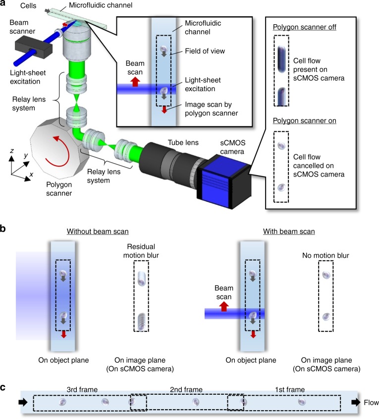
Fig. 1
VIFFI flow cytometry.
a Schematic and functionality. The side inset shows the effect of VIFFI on the formed images of cells on the sCMOS camera. The upper inset shows scanned light-sheet excitation of cells flowing in the ...
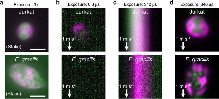
Fig. 2
Demonstration of VIFFI flow cytometry.
Immortalized human T lymphocyte cells (Jurkat) and E. gracilis cells are used for all cases. a Fluorescence images of the cells at rest obtained by conventional fluorescence microscopy. The images are...
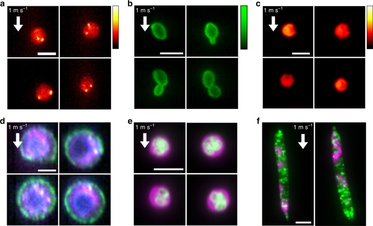
Fig. 3
Fluorescence images of diverse cell types obtained by VIFFI flow cytometry.
All the images were obtained at a flow speed of 1u2009mu2009s u22121 . a FISH images of Jurkat cells. Two bright spots (shown in yellow-white) corresponding to two copies of chromosome 8 are evident i...
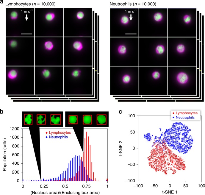
Fig. 4
High-throughput, high-content screening of murine neutrophils, and lymphocytes with VIFFI flow cytometry.
a Libraries of fluorescence images of the cells ( n =u200910,000 for each group) obtained by VIFFI flow cytometry. The cytoplasm was stained by CellTracker Red (shown in magenta) while the nucleus was...
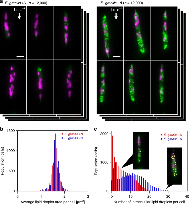
Fig. 5
High-throughput, high-content screening of E. gracilis cells.
a Fluorescence images of nitrogen-sufficient (+N) and nitrogen-deficient (u2212N) E. gracilis cells ( n =u200912,000 for each group) obtained by VIFFI flow cytometry. The lipids (shown in green) were ...
Figure images are served from the NIH/NLM PubMed Central Open Access Subset or Europe PMC; copyright remains with the publishers and authors.
💬 Discussion
0 commentsNo comments yet. Be the first to start a discussion!
Leave a Comment