Abstract
Eukaryotic 60S ribosomal subunits are comprised of three rRNAs and ∼50 ribosomal proteins. The initial steps of their formation take place in the nucleolus, but, owing to a lack of structural information, this process is poorly understood. Using cryo-EM, we solved structures of early 60S biogenesis intermediates at 3.3 Å to 4.5 Å resolution, thereby providing insights into their sequential folding and assembly pathway. Besides revealing distinct immature rRNA conformations, we map 25 assembly factors in six different assembly states. Notably, the Nsa1-Rrp1-Rpf1-Mak16 module stabilizes the solvent side of the 60S subunit, and the Erb1-Ytm1-Nop7 complex organizes and connects through Erb1's meandering N-terminal extension, eight assembly factors, three ribosomal proteins, and three 25S rRNA domains. Our structural snapshots reveal the order of integration and compaction of the six major 60S domains within early nucleolar 60S particles developing stepwise from the solvent side around the exit tunnel to the central protuberance.
🔬 Techniques
🔭 Microscopes
🧬 Organisms
💻 Software
✨ Fluorophores
🧪 Sample Preparation
🏭 Microscope Brands
🧪 Reagent Suppliers
📷 Detectors
💻 Software Details
💾 Data Repositories
🏛️ Research Organizations (ROR)
Affiliated research institutions:
📋 Methods
Key Resources Table REAGENT or RESOURCE SOURCE IDENTIFIER
Bacterial and Virus Strains
E. coli BL21(DE3) Merck 69450 Deposited Data Cryo-EM density map: State A This paper EMD-3888 Cryo-EM density map: State B This paper EMD-3889 Cryo-EM density map: State C This paper EMD-3893 Cryo-EM density map: State D This paper EMD-3890 Cryo-EM density map: State E This paper EMD-3891 Cryo-EM density map: State F This paper EMD-3892 Atomic model: Rrp1 (Spacegroup C2) This paper PDB: 6EMF Atomic model: Rrp1 (Spacegroup P6322) This paper PDB: 6EMG Atomic model: Nsa1 This paper PDB: 6EN7 Atomic model: State C This paper PDB: 6EM1 Atomic model: State E This paper PDB: 6ELZ Architectural model: State A This paper PDB: 6EM3 Architectural model: State B This paper PDB: 6EM4 Architectural model: State D This paper PDB: 6EM5 Experimental Models: Organisms/Strains Yeast: W303 Thomas and Rothstein, 1989 N/A Yeast: DS1-2b Nissan et al., 2002 N/A Yeast: NSA1-TAP Flag-YTM1 This paper N/A Yeast: RIX1-TAP RPF2-Flag This paper N/A Yeast: BRX1-HTpA This paper N/A Yeast: pA-TEV-(HIS)6-RPF1 This paper N/A Recombinant DNA pFA6a-Flag-natNT2 This paper N/A pFA6a-TAP-klURA3 This paper N/A pnatNT2 P YTM1 Flag This paper N/A YCplac111-TAP-Flag-YTM1 Thoms et al., 2016 N/A YCplac111-TAP-Flag-ytm1 ΔUBL This paper N/A YCplac111-TAP-Flag-ytm1 E80A This paper N/A YCplac111-pA-TEV-(His) 6 -RPF1 This paper N/A pET15b-CtRrp1-(His) 6 Baßler et al., 2017 N/A pET15b-Nsa1-(His) 6 This paper N/A Software and Algorithms EM-TOOLS TVIPS GmbH http://www.tvips.com/imaging-software/em-tools/ MotionCorr2.1 Li et al., 2013 http://cryoem.ucsf.edu/software/driftcorr.html GCTF Zhang, 2016 http://www.mrc-lmb.cam.ac.uk/kzhang Motioncor2 Zheng et al., 2017 http://msg.ucsf.edu/em/software/motioncor2.html Gautomatch Jack Kai Zhang, Division of structural studies, MRC Laboratory of Molecular Biology http://www.mrc-lmb.cam.ac.uk/kzhang Relion-2 Kimanius et al., 2016 http://www2.mrc-lmb.cam.ac.uk/relion/index.php/Main_Page Phenix suite (phenix.real_space_refine, molprobity) Afonine et al., 2012 , Chen et al., 2010 , Wang et al., 2014 https://www.phenix-online.org/ PSIPRED UCL Department Of Computer Science http://bioinf.cs.ucl.ac.uk/psipred/ HHpred / Modeler Meier and Söding, 2015 https://toolkit.tuebingen.mpg.de/#/tools/hhpred Phyre2 Kelley et al., 2015 http://www.sbg.bio.ic.ac.uk/∼phyre2 CCP4 (LIBG, ProSMART, Refmac5, Buccaneer, AIMLESS, XDS, Phaser, COOT, SHELXC/D/E) Amunts et al., 2014 , Brown et al., 2015 , Cowtan, 2006 , Emsley et al., 2010 , Evans and Murshudov, 2013 , Kabsch, 2014 , McCoy et al., 2007 , Murshudov et al., 2011 , Winn et al., 2002 , Sheldrick, 2008 http://www.ccp4.ac.uk/ ClustalOMEGA EMBL-EBI https://www.ebi.ac.uk/Tools/msa/clustalo RNAcomposer Institute of Computing Science, Poznan University of Technology http://rnacomposer.ibch.poznan.pl/ Chimera UCSF Resource for Biocomputing, Visualization, and Bioinformatics http://www.cgl.ucsf.edu/chimera/ Pymol PyMOL Molecular Graphics System, Schrödinger, LLC https://pymol.org/2/ HKL2MAP Pape and Schneider, 2004 http://webapps.embl-hamburg.de/hkl2map/ Other Carbon coated holey grids (2nm) R 3/3 Copper Quantifoil N/A Contact for Reagent and Resource Sharing Further information and requests for resources and reagents should be directed to and will be fulfilled by the Lead Contact, Roland Beckmann ( beckmann@lmb.uni-muenchen.de ).
Show full methods section
Key Resources Table REAGENT or RESOURCE SOURCE IDENTIFIER
Bacterial and Virus Strains
E. coli BL21(DE3) Merck 69450 Deposited Data Cryo-EM density map: State A This paper EMD-3888 Cryo-EM density map: State B This paper EMD-3889 Cryo-EM density map: State C This paper EMD-3893 Cryo-EM density map: State D This paper EMD-3890 Cryo-EM density map: State E This paper EMD-3891 Cryo-EM density map: State F This paper EMD-3892 Atomic model: Rrp1 (Spacegroup C2) This paper PDB: 6EMF Atomic model: Rrp1 (Spacegroup P6322) This paper PDB: 6EMG Atomic model: Nsa1 This paper PDB: 6EN7 Atomic model: State C This paper PDB: 6EM1 Atomic model: State E This paper PDB: 6ELZ Architectural model: State A This paper PDB: 6EM3 Architectural model: State B This paper PDB: 6EM4 Architectural model: State D This paper PDB: 6EM5 Experimental Models: Organisms/Strains Yeast: W303 Thomas and Rothstein, 1989 N/A Yeast: DS1-2b Nissan et al., 2002 N/A Yeast: NSA1-TAP Flag-YTM1 This paper N/A Yeast: RIX1-TAP RPF2-Flag This paper N/A Yeast: BRX1-HTpA This paper N/A Yeast: pA-TEV-(HIS)6-RPF1 This paper N/A Recombinant DNA pFA6a-Flag-natNT2 This paper N/A pFA6a-TAP-klURA3 This paper N/A pnatNT2 P YTM1 Flag This paper N/A YCplac111-TAP-Flag-YTM1 Thoms et al., 2016 N/A YCplac111-TAP-Flag-ytm1 ΔUBL This paper N/A YCplac111-TAP-Flag-ytm1 E80A This paper N/A YCplac111-pA-TEV-(His) 6 -RPF1 This paper N/A pET15b-CtRrp1-(His) 6 Baßler et al., 2017 N/A pET15b-Nsa1-(His) 6 This paper N/A Software and Algorithms EM-TOOLS TVIPS GmbH http://www.tvips.com/imaging-software/em-tools/ MotionCorr2.1 Li et al., 2013 http://cryoem.ucsf.edu/software/driftcorr.html GCTF Zhang, 2016 http://www.mrc-lmb.cam.ac.uk/kzhang Motioncor2 Zheng et al., 2017 http://msg.ucsf.edu/em/software/motioncor2.html Gautomatch Jack Kai Zhang, Division of structural studies, MRC Laboratory of Molecular Biology http://www.mrc-lmb.cam.ac.uk/kzhang Relion-2 Kimanius et al., 2016 http://www2.mrc-lmb.cam.ac.uk/relion/index.php/Main_Page Phenix suite (phenix.real_space_refine, molprobity) Afonine et al., 2012 , Chen et al., 2010 , Wang et al., 2014 https://www.phenix-online.org/ PSIPRED UCL Department Of Computer Science http://bioinf.cs.ucl.ac.uk/psipred/ HHpred / Modeler Meier and Söding, 2015 https://toolkit.tuebingen.mpg.de/#/tools/hhpred Phyre2 Kelley et al., 2015 http://www.sbg.bio.ic.ac.uk/∼phyre2 CCP4 (LIBG, ProSMART, Refmac5, Buccaneer, AIMLESS, XDS, Phaser, COOT, SHELXC/D/E) Amunts et al., 2014 , Brown et al., 2015 , Cowtan, 2006 , Emsley et al., 2010 , Evans and Murshudov, 2013 , Kabsch, 2014 , McCoy et al., 2007 , Murshudov et al., 2011 , Winn et al., 2002 , Sheldrick, 2008 http://www.ccp4.ac.uk/ ClustalOMEGA EMBL-EBI https://www.ebi.ac.uk/Tools/msa/clustalo RNAcomposer Institute of Computing Science, Poznan University of Technology http://rnacomposer.ibch.poznan.pl/ Chimera UCSF Resource for Biocomputing, Visualization, and Bioinformatics http://www.cgl.ucsf.edu/chimera/ Pymol PyMOL Molecular Graphics System, Schrödinger, LLC https://pymol.org/2/ HKL2MAP Pape and Schneider, 2004 http://webapps.embl-hamburg.de/hkl2map/ Other Carbon coated holey grids (2nm) R 3/3 Copper Quantifoil N/A Contact for Reagent and Resource Sharing Further information and requests for resources and reagents should be directed to and will be fulfilled by the Lead Contact, Roland Beckmann ( beckmann@lmb.uni-muenchen.de ).
Experimental Model and Subject Details
Plasmid constructs and yeast strains Recombinant
DNA techniques were performed using standard procedures. Cloning and plasmid propagation was carried out with E. coli DH5α. Cloned DNA fragments obtained by PCR amplification were verified through sequencing. Plasmids used in this study are listed in Table S1 . S. cerevisiae strains used and generated in this study are listed in Table S2 . Genomic tagging was performed as previously described according to standard procedures ( Janke et al., 2004 , Longtine et al., 1998 ). Method Details Affinity purifications from S. cerevisiae The NSA1 -TAP Flag- YTM1 and the RIX1 -TAP RPF2 -Flag strains were grown in YPD medium and harvested at an OD 600 of 2.0-2.5. For the YTM1 wild-type, ytm1 ΔUBL and ytm1 E80A alleles plasmids were generated harboring the respective coding sequences fused to an N-terminal TAP-Flag tag under control of the endogenous P YTM1 promoter. The plasmids were transformed into a wild-type strain (W303) ( Thomas and Rothstein, 1989 ) and selected on SDC-Leu. Cultures were grown over-night in SDC-Leu medium and shifted to YPD for additional 6-7 h until the cultures reached an OD 600 of 2.0-2.5. Cell pellets were harvested by centrifugation, flash frozen in liquid nitrogen and stored at −20°C. The affinity purifications were performed as described previously ( Barrio-Garcia et al., 2016 ). Cells were disrupted by cryogenic grinding with a Retch grinding mill (MM 400) and the cell powder was incubated with lysis buffer containing 50 mM Tris pH 7.5, 100 mM NaCl, 5 mM MgCl 2 , 5% (v/v) glycerol, 1 mM DTT and 0.1% (w/v) NP40 supplemented with protease inhibitors (SIGMAFAST, Sigma Aldrich). The lysate was cleared by centrifugation and incubated with IgG Sepharose 6 Fast Flow (GE Healthcare) for 90 min at 4°C to enrich for the TAP tagged bait protein. Beads were collected and washed once with 25 mL lysis buffer (batch wash) and additionally with 10 mL lysis buffer by gravity flow. The IgG beads were collected and incubated with lysis buffer supplemented with TEV protease to release the sample from the beads. The eluate was incubated with Anti-Flag M2 Affinity gel (Sigma Aldrich) for additional 90 min at 4°C to enrich for the Flag tagged protein. The remaining steps were performed in buffer containing 50 mM Tris pH 7.5, 100 mM NaCl, 5 mM MgCl 2 and 1 mM DTT. The Flag agarose beads were extensively washed and samples were eluted with ca. 60 μl buffer supplemented with Flag peptide. Protein production, crystallization and structure determination ScNsa1 For expression of Saccharomyces cerevisiae ( Sc ) Nsa1-(His) 6 , E. coli BL21(DE3) cells, grown in lysogeny broth (LB) medium, were used. Protein expression was induced with 1.8% (w/v) lactose, and cells were harvested after overnight growth at 30°C and stored at −80°C. Cells pellets were resuspended in 10 mL buffer A (20mM HEPES (pH 8.0), 250mM NaCl, 20mM KCl, 20mM MgCl2 and 40mM imidazole) per gram of cells and lysed with a M-110L Microfluidizer (Microfluidics). Lysate was cleared at 20,000 r.p.m and Nsa1 was enriched by Ni-NTA chromatography. Nsa1 was eluted from Ni-NTA by buffer B (20mM HEPES (pH 8.0), 250mM NaCl, 20mM KCl, 20mM MgCl 2 , 500mM imidazole) and further purified by size-exclusion chromatography (HiLoad 26/60 Superdex 200) equilibrated in buffer C (20mM HEPES (pH 8), 200mM NaCl, 20mM KCl and 20mM MgCl 2 ). Protein was concentrated to approximately 30 mg/ml and crystallization screens were performed at 291K by the sitting-drop vapor-diffusion method upon mixing equal volumes (0.5 μl) of protein solution and crystallization buffer with a reservoir volume of 100 μl. Nsa1 crystallized in a wide range of polyethyleneglycol (PEG)-containing conditions (e.g., 0.1 M MES pH 6.5, 25% w/v PEG-1000). Prior data collection, crystals were flash-frozen in liquid nitrogen after cryo-protection by transfer into cryo-solution containing mother liquor and 20% (v/v) glycerol. Diffraction data were measured under cryogenic conditions (100 K; Oxford Cryosystems Cryostream) at the European Synchrotron Radiation Facility (ESRF; Grenoble). Data were processed with XDS ( Kabsch, 2014 ). The Nsa1 structure was determined by molecular replacement using PHASER and PDB: 5SUM as search model. The structure was manually corrected with Coot ( Emsley et al., 2010 ) and refined with REFMAC5 ( Murshudov et al., 2011 ) and PHENIX ( Afonine et al., 2012 ). Data collection and refinement statistics are summarized in Table S3 . CtRrp1 Rrp1 from Chaetomium thermophilum ( Ct ) was expressed in Rosetta 2 (DE3) T1R cells transformed with the pET15b-CtRrp1-(His) 6 plasmid ( Baßler et al., 2017 ). Briefly, cells were grown until an OD 600 of 0.8 was reached and then transferred to 18°C. Protein expression was induced by the addition of 0.5 mM IPTG and cells were further grown overnight. Harvested cells were lysed in buffer L (30 mM HEPES pH7.5, 30 mM imidazole, 500 mM NaCl) using a Microfludizer (Microfluidics). Cell debris and insoluble proteins were removed by centrifugation for 35 minutes at 35000 × g and 4°C. The cleared lysate was filtered with 0.45 μm filter and applied to 2 mL NiNTA column. After washing with 30 column volumes with buffer L the protein was eluted using buffer H (buffer L plus 400 mM Imidazol). Further purification was done using a Superdex 75 26/60 column equilibrated with buffer S (20 mM HEPES pH 7.5, 400 mM NaCl, 5 mM MgCl 2 , 2 mM DTT). Ct Rrp1 containing fractions were pooled, concentrated to 20-40 mg/ml and used for crystallization trials. Ct Rrp1 crystallized in two conditions, giving rod-shaped crystals in PEG-3350 based condition (200 mM Proline, 100 mM HEPES pH 7.5, 10% PEG3350) and thick hexagonal shaped crystals in a phosphate-containing condition (0.8M K-H 2 PO 4 , 0.8M Na-H 2 PO 4 ). For data-collection crystals from both conditions were harvested into reservoir solution supplemented with 20% glycerol or ethylene-glycol and flash cooled in liquid nitrogen. Data were collected at ESRF beamline ID 29 ( de Sanctis et al., 2012 ). For phasing, a crystal from the phosphate condition was soaked in reservoir solution supplemented with 1 mM K 2 PtCl 4 for 1 hour and cryo-protected as described above. Data were collected at ESRF beamline ID29. Data were processed with XDS ( Kabsch, 2014 ) and AIMLESS ( Evans and Murshudov, 2013 ) from the CCP4 package ( Winn et al., 2002 ). The structure was solved with SHELXC/D/E ( Sheldrick, 2008 ) navigated with HKL2MAP ( Pape and Schneider, 2004 ). The initial map was readily interpretable and Buccaneer ( Cowtan, 2006 ) could place the majority of the residues automatically. Remaining residues were built with Coot ( Emsley et al., 2010 ) and the structure was refined with REFMAC5 ( Murshudov et al., 2011 ) and PHENIX ( Afonine et al., 2012 ). The C 2-dataset was solved by molecular replacement as implemented in PHASER ( McCoy et al., 2007 )], using the previously determined structure as search model. The final structures contain 2 molecules per ASU in both space-groups, arranged in different way to each other. Data collection and refinement statistics are summarized in Table S4 . CRAC analysis The CRAC experiments for Brx1 and Rpf1 were done as described in Granneman et al. (2009) and Thoms et al. (2015) with a modification in case of Rpf1. Brx1 was tagged at the C terminus with (HIS) 6 -TEV-protA (HTpA). Rpf1 was tagged at the N terminus on a plasmid (YCplac111- pA-TEV-(HIS) 6 -RPF1). Untagged W303 was used as a background control. The yeast cultures were grown to OD 0.6-0.7 and UV-irradiated ( in vivo ) using a Megatron chamber (1.6 J/cm 2 ). Brx1 and Rpf1 were purified as described in Granneman et al. (2009) including high salt (1M NaCl) wash after IgG purification. For Brx1, the sample was transferred to nitrocellulose membrane and RNA was extracted from the membrane as described in Granneman et al. (2009) . In case of Rpf1, RNA was extracted directly from the imidazole eluate. For both proteins, the cDNAs obtained were sequenced using the Illumina MiSeq sequencing platform. Analysis of the sequencing results was done as described in Thoms et al. (2015) . The 5′ and 3′ linkers, RT and PCR oligos are listed in Table S6 ( Thoms et al., 2015 ). The experiments were performed twice for both proteins and the results were reproducible.
Cryo-electron microscopy
Carbon coated holey grids (2nm, Quantifoil) were glow discharged at 2.2x10 −1 mbar for 30 s. For each grid, 3.5μl of sample were applied to the grids at a concentration of 1.8 A 260 ml -1 for the Nsa1-TAP Flag-Ytm1 sample, 1.5 A 260 ml -1 for the TAP-Flag-Ytm1 E80A sample and 1.3 A 260 ml -1 for the Rix1-TAP Rpf2-Flag sample. Subsequent vitrification was performed by plunge freezing in liquid ethane using a Vitrobot mark IV (FEI Company, Netherlands) with a blotting time of 3 s at 4°C. Cryo-EM data were collected semi-automatically using the acquisition software EM-TOOLS (TVIPS, Germany) on a Titan Krios transmission electron microscope (FEI Company) at a defocus range between 0.9 and 3.5 μm. All data for the Nsa1-TAP Flag-Ytm1 sample and the Rix1-TAP Rpf2-Flag sample were recorded on a Falcon II detector under low dose conditions with a nominal pixel size of 1.084 A/pixel on the object scale. For the Nsa1-TAP Flag-Ytm1 sample, a total of four datasets comprising 2547, 689, 1196 and 1046 micrographs were collected. All micrographs experienced a total exposure of ∼27 e − /A 2 fractionated into 6 frames for the first dataset and 10 for all subsequent datasets. For the Rix1-Tap Rpf2-Flag sample 4447 micrographs dose fractionated into 10 frames were collected. Micrographs of the TAP-Flag-Ytm1 E80A sample were recorded using a Falcon II upgraded with a Falcon III detector chip also operating with a pixel size of 1.084 Å/pixel on the object scale. For this dataset 5812 micrographs were collected with an accumulated dose of 27e − /Å fractionated into 10 frames.
Image processing
Dose-fractionation movies were initially aligned and summed up using MotionCorr2.1 ( Li et al., 2013 ). Determination of the contrast transfer function parameters was performed via GCTF ( Zhang, 2016 ). For further processing, the original movies were re-aligned with Motioncor2 with anisotropic motion correction ( Zheng et al., 2017 ) using 5x5 patches. Gautomatch ( http://www.mrc-lmb.cam.ac.uk/kzhang ) was used to pick particles. All further image processing (classifications, refinements, and particle polishing) was performed using Relion-2.0 ( Kimanius et al., 2016 ).
Nsa1-TAP Flag-Ytm1 dataset
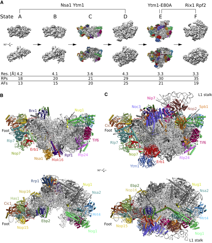
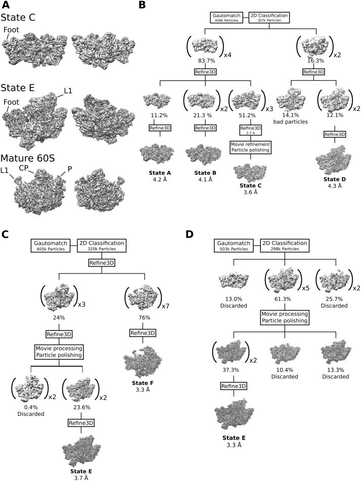
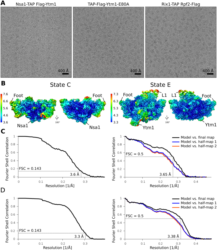
First, all picked particles were subjected to two-dimensional reference free classification into 150 classes. Based on the resulting class averages, 90 classes with a total of 306732 particles were selected for further processing. An initial round of 3D classification was performed using the Arx1 particle (EMDB: 2528) as a reference allowing rotational and translational alignment. Classes with similar map features were combined, subjected to 3D refinement and second rounds of 3D-classifications. After the final classification step, similar maps classes were joined and 3D-refinements using a wide soft edge mask and solvent flattened FSC calculation were performed. Particles of the highest resolved state C (3.7 Å) were then subjected to movie refinement of individual particle stacks using a running average window of 3 frames and a standard deviation of 1 pixel as a prior for the translations ( Bai et al., 2013 ). Particle polishing ( Scheres, 2014 ) was performed using default parameters, followed by a final round of 3D refinement. All final reconstructions were subjected to post processing using a wide soft edge mask. In this fashion, four distinct states were recovered from the dataset, State A at a resolution of 4.2 Å, State B at 4.1 Å, State C at 3.6 Å and State D at 4.3 Å. All resolutions are supplied according to the FSC 0.143 criterion following the Relion gold-standard refinement ( Figure S2 ).
Rix1-TAP Rpf2-Flag dataset
Reference free two dimensional classification into 150 classes yielded in 60 classes with 320144 good (ribosomal) particles. These were subjected to 3D refinement and classified into 10 classes. Based on visual inspection of the map features, classes were combined and further refined. Movie processing and particle polishing was performed as described above. Another round of 3D classification followed by a final 3D refinement and post-processing yields in State E with a nominal resolution of 3.7 Å. The remaining 7 classes of the initial 3D classification were all joined and refined, resulting in state F with an average resolution of 3.3 Å after post processing with a wide soft edge mask ( Figure S2 ).
TAP-Flag-YtmE80A dataset
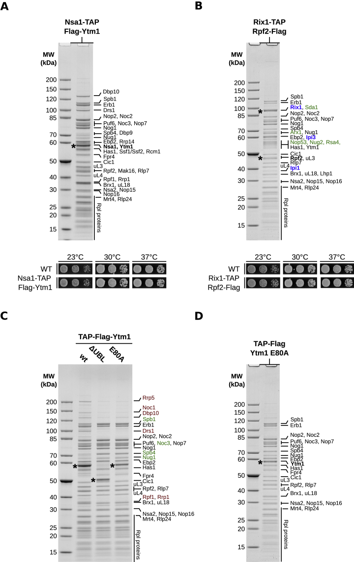
All particles were subjected to reference free 2D classification into 200 classes, yielding 78 classes with 297516 good ribosomal particles. After an initial round of 3D refinement, 3D classification of the particles into 8 classes was performed. The 5 classes representing the state E of the Rix1-TAP Rpf2-Flag sample were joined. Movie processing and particle polishing was performed as described above. A further round of 3D classification was performed followed by a final round of 3D refinement yielding a 3.3 Å reconstruction of state E after post processing with a wide soft edge mask ( Figure S2 ). Model building and refinements Based on the proteins identified in the purification ( Figure S1 ), a model was built for the Ytm1 E80A state E map. Therefore, the model of the Nog2 particle (PDB: 3jct ) was first fitted as a rigid body into the State E density using UCSF Chimera ( Pettersen et al., 2004 ). This served as a starting model for fitting the ribosomal RNA, the RPs as well as the biogenesis factors Cic1, Mrt4, Nog1, Nop7, Nop15, Nsa2, Nug1, Rlp24, Rlp7 and Tif6. Chains of factors not represented by density in this map were deleted, the rRNA stretches that were not represented by the density were pruned. The results were then manually inspected and adjusted in COOT ( Emsley et al., 2010 ). Nucleotides 2404-2818 were independently fitted with COOT based on the crystal structure of the yeast 80S ribosome (PDB: 4V7R ). For target proteins with existing homologies, secondary structure predictions were calculated by PSIPRED and homology models were created via HHpred/Modeler ( Meier and Söding, 2015 ) and Phyre2 ( Kelley et al., 2015 ). The homology models then served as a starting model for de-novo building in COOT. Assignments of the proteins were confirmed by side chain density and secondary structure patterns. Assignments of the structurally similar Brix proteins were verified using CRAC analysis ( Figure S6 ). All models were combined and subsequently refined using phenix.real_space_refine ( Wang et al., 2014 ). Refmac5 reciprocal space refinement using restraints generated via LIBG and ProSMART was then performed as previously shown ( Amunts et al., 2014 , Brown et al., 2015 ). The model for Nsa1-TAP Flag-Ytm1 state C was created as previously described, the final model of state E was used as a starting model. The crystal structure of Nsa1 (this study) ( Figure S6 B) was used as a starting model and modified in COOT. An S. cerevisiae homology model of Rrp1 was created using MODELER with the C. thermophilum crystal structure (also this study) ( Figure S6 C) and the respective sequence alignment from ClustalOMEGA as input. For modeling the RNA of ES7a, an RNA tertiary structure prediction by RNAComposer ( http://rnacomposer.ibch.poznan.pl/ ) was used as an initial reference. Refinement of the model was performed as described for Ytm1 E80A state E, with the exception that the chains of the less well resolved “foot” region (ITS2 RNA, Cic1/Nsa3, Erb1, Has1, Nop7, Nop15 and Rlp7) were not subjected to refinement in Refmac5 but docked as a rigid body using chimera. Architectural models of states A, B and D were created on the basis of the refined state C and E models. First a general model was created by clipping segments not represented by the respective density map using chimera, the chains of the resulting model were then rigid body fitted using phenix.real_space_refine and finally sidechains were removed using phenix.pdbtools ( Pettersen et al., 2004 , Wang et al., 2014 ). Values of the final refinements and model validation for both models are provided in Table S5 . Molecular interpretation of State F was based on the Arx1/Nog2 particle model (PDB: 3JCT ) ( Wu et al., 2016 ). Figures were created using UCSF chimera and PyMOL Molecular Graphics System (Version 1.7.4, Schrödinger, LLC).
Quantification and Statistical Analyses See Methods
Details for details on image processing and model building and refinements.
Data and Software Availability
All maps are deposited at EMDB as noted in the Key Resources Table . Atomic models and architectural models are deposited at PDB as noted in the Key Resources Table . Accession codes Cryo-EM density map State A-F: EMDB: EMD-3888; EMDB: EMD-3889; EMDB: EMD-3893; EMDB: EMD-3890; EMDB: EMD-3891; EMDB: EMD-3892 Atomic model (PDB) Rrp1 (Spacegroup C2, P6322): PDB: 6EMF , PDB: 6EMG Atomic model (PDB) Nsa1: PDB: 6EN7 Atomic model (PDB) State C, E: PDB: 6EM1 , PDB: 6ELZ Architectural model (PDB) state A, B, D: PDB: 6EM3 , PDB: 6EM4 , PDB: 6EM5
Experimental Model and Subject Details
Plasmid constructs and yeast strains Recombinant
DNA techniques were performed using standard procedures. Cloning and plasmid propagation was carried out with E. coli DH5α. Cloned DNA fragments obtained by PCR amplification were verified through sequencing. Plasmids used in this study are listed in Table S1 . S. cerevisiae strains used and generated in this study are listed in Table S2 . Genomic tagging was performed as previously described according to standard procedures ( Janke et al., 2004 , Longtine et al., 1998 ).
Method Details Affinity purifications from S. cerevisiae The NSA1 -TAP Flag- YTM1 and the RIX1 -TAP RPF2 -Flag strains were grown in YPD medium and harvested at an OD 600 of 2.0-2.5. For the YTM1 wild-type, ytm1 ΔUBL and ytm1 E80A alleles plasmids were generated harboring the respective coding sequences fused to an N-terminal TAP-Flag tag under control of the endogenous P YTM1 promoter. The plasmids were transformed into a wild-type strain (W303) ( Thomas and Rothstein, 1989 ) and selected on SDC-Leu. Cultures were grown over-night in SDC-Leu medium and shifted to YPD for additional 6-7 h until the cultures reached an OD 600 of 2.0-2.5. Cell pellets were harvested by centrifugation, flash frozen in liquid nitrogen and stored at −20°C. The affinity purifications were performed as described previously ( Barrio-Garcia et al., 2016 ). Cells were disrupted by cryogenic grinding with a Retch grinding mill (MM 400) and the cell powder was incubated with lysis buffer containing 50 mM Tris pH 7.5, 100 mM NaCl, 5 mM MgCl 2 , 5% (v/v) glycerol, 1 mM DTT and 0.1% (w/v) NP40 supplemented with protease inhibitors (SIGMAFAST, Sigma Aldrich). The lysate was cleared by centrifugation and incubated with IgG Sepharose 6 Fast Flow (GE Healthcare) for 90 min at 4°C to enrich for the TAP tagged bait protein. Beads were collected and washed once with 25 mL lysis buffer (batch wash) and additionally with 10 mL lysis buffer by gravity flow. The IgG beads were collected and incubated with lysis buffer supplemented with TEV protease to release the sample from the beads. The eluate was incubated with Anti-Flag M2 Affinity gel (Sigma Aldrich) for additional 90 min at 4°C to enrich for the Flag tagged protein. The remaining steps were performed in buffer containing 50 mM Tris pH 7.5, 100 mM NaCl, 5 mM MgCl 2 and 1 mM DTT. The Flag agarose beads were extensively washed and samples were eluted with ca. 60 μl buffer supplemented with Flag peptide. Protein production, crystallization and structure determination ScNsa1 For expression of Saccharomyces cerevisiae ( Sc ) Nsa1-(His) 6 , E. coli BL21(DE3) cells, grown in lysogeny broth (LB) medium, were used. Protein expression was induced with 1.8% (w/v) lactose, and cells were harvested after overnight growth at 30°C and stored at −80°C. Cells pellets were resuspended in 10 mL buffer A (20mM HEPES (pH 8.0), 250mM NaCl, 20mM KCl, 20mM MgCl2 and 40mM imidazole) per gram of cells and lysed with a M-110L Microfluidizer (Microfluidics). Lysate was cleared at 20,000 r.p.m and Nsa1 was enriched by Ni-NTA chromatography. Nsa1 was eluted from Ni-NTA by buffer B (20mM HEPES (pH 8.0), 250mM NaCl, 20mM KCl, 20mM MgCl 2 , 500mM imidazole) and further purified by size-exclusion chromatography (HiLoad 26/60 Superdex 200) equilibrated in buffer C (20mM HEPES (pH 8), 200mM NaCl, 20mM KCl and 20mM MgCl 2 ). Protein was concentrated to approximately 30 mg/ml and crystallization screens were performed at 291K by the sitting-drop vapor-diffusion method upon mixing equal volumes (0.5 μl) of protein solution and crystallization buffer with a reservoir volume of 100 μl. Nsa1 crystallized in a wide range of polyethyleneglycol (PEG)-containing conditions (e.g., 0.1 M MES pH 6.5, 25% w/v PEG-1000). Prior data collection, crystals were flash-frozen in liquid nitrogen after cryo-protection by transfer into cryo-solution containing mother liquor and 20% (v/v) glycerol. Diffraction data were measured under cryogenic conditions (100 K; Oxford Cryosystems Cryostream) at the European Synchrotron Radiation Facility (ESRF; Grenoble). Data were processed with XDS ( Kabsch, 2014 ). The Nsa1 structure was determined by molecular replacement using PHASER and PDB: 5SUM as search model. The structure was manually corrected with Coot ( Emsley et al., 2010 ) and refined with REFMAC5 ( Murshudov et al., 2011 ) and PHENIX ( Afonine et al., 2012 ). Data collection and refinement statistics are summarized in Table S3 . CtRrp1 Rrp1 from Chaetomium thermophilum ( Ct ) was expressed in Rosetta 2 (DE3) T1R cells transformed with the pET15b-CtRrp1-(His) 6 plasmid ( Baßler et al., 2017 ). Briefly, cells were grown until an OD 600 of 0.8 was reached and then transferred to 18°C. Protein expression was induced by the addition of 0.5 mM IPTG and cells were further grown overnight. Harvested cells were lysed in buffer L (30 mM HEPES pH7.5, 30 mM imidazole, 500 mM NaCl) using a Microfludizer (Microfluidics). Cell debris and insoluble proteins were removed by centrifugation for 35 minutes at 35000 × g and 4°C. The cleared lysate was filtered with 0.45 μm filter and applied to 2 mL NiNTA column. After washing with 30 column volumes with buffer L the protein was eluted using buffer H (buffer L plus 400 mM Imidazol). Further purification was done using a Superdex 75 26/60 column equilibrated with buffer S (20 mM HEPES pH 7.5, 400 mM NaCl, 5 mM MgCl 2 , 2 mM DTT). Ct Rrp1 containing fractions were pooled, concentrated to 20-40 mg/ml and used for crystallization trials. Ct Rrp1 crystallized in two conditions, giving rod-shaped crystals in PEG-3350 based condition (200 mM Proline, 100 mM HEPES pH 7.5, 10% PEG3350) and thick hexagonal shaped crystals in a phosphate-containing condition (0.8M K-H 2 PO 4 , 0.8M Na-H 2 PO 4 ). For data-collection crystals from both conditions were harvested into reservoir solution supplemented with 20% glycerol or ethylene-glycol and flash cooled in liquid nitrogen. Data were collected at ESRF beamline ID 29 ( de Sanctis et al., 2012 ). For phasing, a crystal from the phosphate condition was soaked in reservoir solution supplemented with 1 mM K 2 PtCl 4 for 1 hour and cryo-protected as described above. Data were collected at ESRF beamline ID29. Data were processed with XDS ( Kabsch, 2014 ) and AIMLESS ( Evans and Murshudov, 2013 ) from the CCP4 package ( Winn et al., 2002 ). The structure was solved with SHELXC/D/E ( Sheldrick, 2008 ) navigated with HKL2MAP ( Pape and Schneider, 2004 ). The initial map was readily interpretable and Buccaneer ( Cowtan, 2006 ) could place the majority of the residues automatically. Remaining residues were built with Coot ( Emsley et al., 2010 ) and the structure was refined with REFMAC5 ( Murshudov et al., 2011 ) and PHENIX ( Afonine et al., 2012 ). The C 2-dataset was solved by molecular replacement as implemented in PHASER ( McCoy et al., 2007 )], using the previously determined structure as search model. The final structures contain 2 molecules per ASU in both space-groups, arranged in different way to each other. Data collection and refinement statistics are summarized in Table S4 . CRAC analysis The CRAC experiments for Brx1 and Rpf1 were done as described in Granneman et al. (2009) and Thoms et al. (2015) with a modification in case of Rpf1. Brx1 was tagged at the C terminus with (HIS) 6 -TEV-protA (HTpA). Rpf1 was tagged at the N terminus on a plasmid (YCplac111- pA-TEV-(HIS) 6 -RPF1). Untagged W303 was used as a background control. The yeast cultures were grown to OD 0.6-0.7 and UV-irradiated ( in vivo ) using a Megatron chamber (1.6 J/cm 2 ). Brx1 and Rpf1 were purified as described in Granneman et al. (2009) including high salt (1M NaCl) wash after IgG purification. For Brx1, the sample was transferred to nitrocellulose membrane and RNA was extracted from the membrane as described in Granneman et al. (2009) . In case of Rpf1, RNA was extracted directly from the imidazole eluate. For both proteins, the cDNAs obtained were sequenced using the Illumina MiSeq sequencing platform. Analysis of the sequencing results was done as described in Thoms et al. (2015) . The 5′ and 3′ linkers, RT and PCR oligos are listed in Table S6 ( Thoms et al., 2015 ). The experiments were performed twice for both proteins and the results were reproducible.
Cryo-electron microscopy
Carbon coated holey grids (2nm, Quantifoil) were glow discharged at 2.2x10 −1 mbar for 30 s. For each grid, 3.5μl of sample were applied to the grids at a concentration of 1.8 A 260 ml -1 for the Nsa1-TAP Flag-Ytm1 sample, 1.5 A 260 ml -1 for the TAP-Flag-Ytm1 E80A sample and 1.3 A 260 ml -1 for the Rix1-TAP Rpf2-Flag sample. Subsequent vitrification was performed by plunge freezing in liquid ethane using a Vitrobot mark IV (FEI Company, Netherlands) with a blotting time of 3 s at 4°C. Cryo-EM data were collected semi-automatically using the acquisition software EM-TOOLS (TVIPS, Germany) on a Titan Krios transmission electron microscope (FEI Company) at a defocus range between 0.9 and 3.5 μm. All data for the Nsa1-TAP Flag-Ytm1 sample and the Rix1-TAP Rpf2-Flag sample were recorded on a Falcon II detector under low dose conditions with a nominal pixel size of 1.084 A/pixel on the object scale. For the Nsa1-TAP Flag-Ytm1 sample, a total of four datasets comprising 2547, 689, 1196 and 1046 micrographs were collected. All micrographs experienced a total exposure of ∼27 e − /A 2 fractionated into 6 frames for the first dataset and 10 for all subsequent datasets. For the Rix1-Tap Rpf2-Flag sample 4447 micrographs dose fractionated into 10 frames were collected. Micrographs of the TAP-Flag-Ytm1 E80A sample were recorded using a Falcon II upgraded with a Falcon III detector chip also operating with a pixel size of 1.084 Å/pixel on the object scale. For this dataset 5812 micrographs were collected with an accumulated dose of 27e − /Å fractionated into 10 frames.
Image processing
Dose-fractionation movies were initially aligned and summed up using MotionCorr2.1 ( Li et al., 2013 ). Determination of the contrast transfer function parameters was performed via GCTF ( Zhang, 2016 ). For further processing, the original movies were re-aligned with Motioncor2 with anisotropic motion correction ( Zheng et al., 2017 ) using 5x5 patches. Gautomatch ( http://www.mrc-lmb.cam.ac.uk/kzhang ) was used to pick particles. All further image processing (classifications, refinements, and particle polishing) was performed using Relion-2.0 ( Kimanius et al., 2016 ).
Nsa1-TAP Flag-Ytm1 dataset
First, all picked particles were subjected to two-dimensional reference free classification into 150 classes. Based on the resulting class averages, 90 classes with a total of 306732 particles were selected for further processing. An initial round of 3D classification was performed using the Arx1 particle (EMDB: 2528) as a reference allowing rotational and translational alignment. Classes with similar map features were combined, subjected to 3D refinement and second rounds of 3D-classifications. After the final classification step, similar maps classes were joined and 3D-refinements using a wide soft edge mask and solvent flattened FSC calculation were performed. Particles of the highest resolved state C (3.7 Å) were then subjected to movie refinement of individual particle stacks using a running average window of 3 frames and a standard deviation of 1 pixel as a prior for the translations ( Bai et al., 2013 ). Particle polishing ( Scheres, 2014 ) was performed using default parameters, followed by a final round of 3D refinement. All final reconstructions were subjected to post processing using a wide soft edge mask. In this fashion, four distinct states were recovered from the dataset, State A at a resolution of 4.2 Å, State B at 4.1 Å, State C at 3.6 Å and State D at 4.3 Å. All resolutions are supplied according to the FSC 0.143 criterion following the Relion gold-standard refinement ( Figure S2 ).
Rix1-TAP Rpf2-Flag dataset
Reference free two dimensional classification into 150 classes yielded in 60 classes with 320144 good (ribosomal) particles. These were subjected to 3D refinement and classified into 10 classes. Based on visual inspection of the map features, classes were combined and further refined. Movie processing and particle polishing was performed as described above. Another round of 3D classification followed by a final 3D refinement and post-processing yields in State E with a nominal resolution of 3.7 Å. The remaining 7 classes of the initial 3D classification were all joined and refined, resulting in state F with an average resolution of 3.3 Å after post processing with a wide soft edge mask ( Figure S2 ).
TAP-Flag-YtmE80A dataset
All particles were subjected to reference free 2D classification into 200 classes, yielding 78 classes with 297516 good ribosomal particles. After an initial round of 3D refinement, 3D classification of the particles into 8 classes was performed. The 5 classes representing the state E of the Rix1-TAP Rpf2-Flag sample were joined. Movie processing and particle polishing was performed as described above. A further round of 3D classification was performed followed by a final round of 3D refinement yielding a 3.3 Å reconstruction of state E after post processing with a wide soft edge mask ( Figure S2 ). Model building and refinements Based on the proteins identified in the purification ( Figure S1 ), a model was built for the Ytm1 E80A state E map. Therefore, the model of the Nog2 particle (PDB: 3jct ) was first fitted as a rigid body into the State E density using UCSF Chimera ( Pettersen et al., 2004 ). This served as a starting model for fitting the ribosomal RNA, the RPs as well as the biogenesis factors Cic1, Mrt4, Nog1, Nop7, Nop15, Nsa2, Nug1, Rlp24, Rlp7 and Tif6. Chains of factors not represented by density in this map were deleted, the rRNA stretches that were not represented by the density were pruned. The results were then manually inspected and adjusted in COOT ( Emsley et al., 2010 ). Nucleotides 2404-2818 were independently fitted with COOT based on the crystal structure of the yeast 80S ribosome (PDB: 4V7R ). For target proteins with existing homologies, secondary structure predictions were calculated by PSIPRED and homology models were created via HHpred/Modeler ( Meier and Söding, 2015 ) and Phyre2 ( Kelley et al., 2015 ). The homology models then served as a starting model for de-novo building in COOT. Assignments of the proteins were confirmed by side chain density and secondary structure patterns. Assignments of the structurally similar Brix proteins were verified using CRAC analysis ( Figure S6 ). All models were combined and subsequently refined using phenix.real_space_refine ( Wang et al., 2014 ). Refmac5 reciprocal space refinement using restraints generated via LIBG and ProSMART was then performed as previously shown ( Amunts et al., 2014 , Brown et al., 2015 ). The model for Nsa1-TAP Flag-Ytm1 state C was created as previously described, the final model of state E was used as a starting model. The crystal structure of Nsa1 (this study) ( Figure S6 B) was used as a starting model and modified in COOT. An S. cerevisiae homology model of Rrp1 was created using MODELER with the C. thermophilum crystal structure (also this study) ( Figure S6 C) and the respective sequence alignment from ClustalOMEGA as input. For modeling the RNA of ES7a, an RNA tertiary structure prediction by RNAComposer ( http://rnacomposer.ibch.poznan.pl/ ) was used as an initial reference. Refinement of the model was performed as described for Ytm1 E80A state E, with the exception that the chains of the less well resolved “foot” region (ITS2 RNA, Cic1/Nsa3, Erb1, Has1, Nop7, Nop15 and Rlp7) were not subjected to refinement in Refmac5 but docked as a rigid body using chimera. Architectural models of states A, B and D were created on the basis of the refined state C and E models. First a general model was created by clipping segments not represented by the respective density map using chimera, the chains of the resulting model were then rigid body fitted using phenix.real_space_refine and finally sidechains were removed using phenix.pdbtools ( Pettersen et al., 2004 , Wang et al., 2014 ). Values of the final refinements and model validation for both models are provided in Table S5 . Molecular interpretation of State F was based on the Arx1/Nog2 particle model (PDB: 3JCT ) ( Wu et al., 2016 ). Figures were created using UCSF chimera and PyMOL Molecular Graphics System (Version 1.7.4, Schrödinger, LLC).
📊 Figures
Figureu00a01
Cryo-EM Structures of Nucleolar Pre-60S Assembly Intermediates (A) Cryo-EM densities filtered to 10u00a0u00c5 in the case of states A, B, D, and F. Maps of states C and E are filtered to 3.6u00a0u00c5...
Figureu00a0S1
Affinity Purification of Nucleolar Pre-60S Particles for Cryo-EM Analysis, Related to Figureu00a01 (A and B) Split affinity purifications of pre-60S intermediates (upper panels) purified through Nsa1-...
Figureu00a0S2
Comparison of States C and E to the Mature 60S and Cryo-EM Processing Schemes, Related to Figureu00a01 (A) Pre-60S States C and D and the mature 60S (EMDB: 6478) ( Passos and Lyumkis, 2015 ) showing t...
Figureu00a0S3
Resolution Estimation and Model Validation, Related to Figureu00a01 (A) Exemplary micrographs of the three different biochemical samples. (Bu2013D) Two views rotated by 180u00b0 of volumes of state C ...
Figureu00a0S4
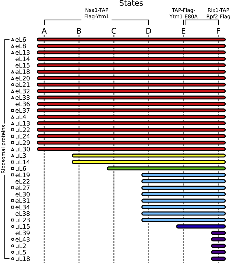
RP Composition of the Six Identified States, Related to Figureu00a01 RPs clustered and colored according to time of stable association with the core particle. RPs are marked with a triangle, square or...
Figureu00a0S5
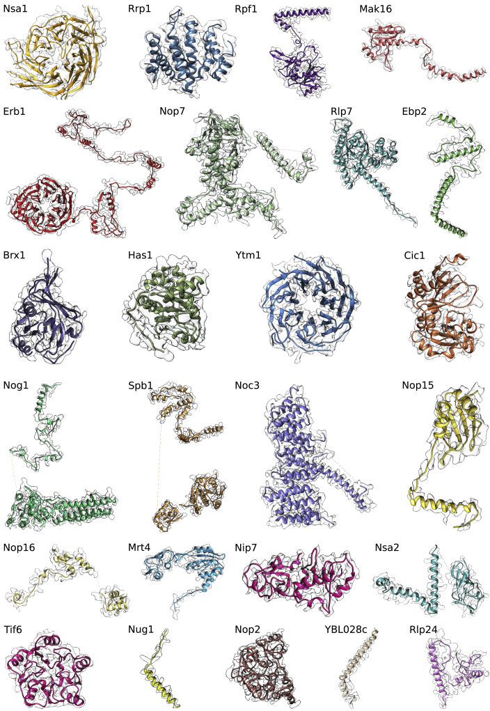
Gallery of All Modeled AFs, Related to Figures 1 , 2 , 3 , and 4 AF models overlaid with the corresponding segmented map volumes. All AFs are taken from state E, except for Rrp1, Rpf1, Nsa1, and Mak16...
Figureu00a0S6
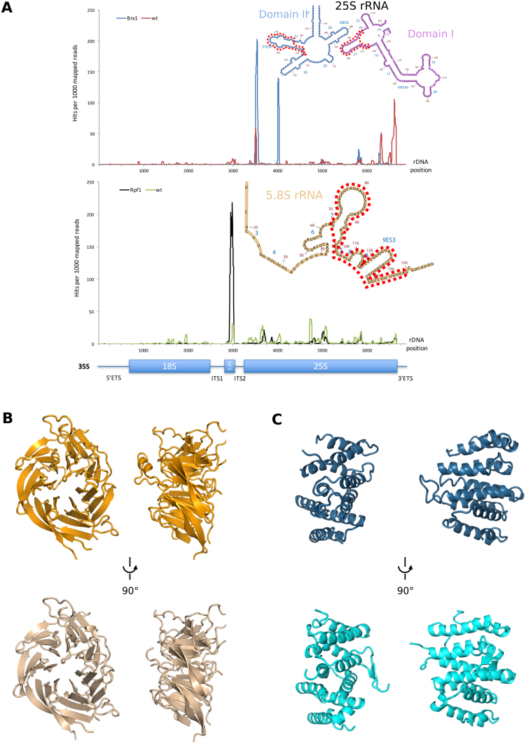
CRAC Crosslinks and Crystal Structures, Related to Figureu00a02 (A) CRAC analysis hits of yeast Brx1 (blue, top plot) and untagged wild-type strain (red, top plot) as well as Rpf1 (black, bottom plot)...
Figureu00a02
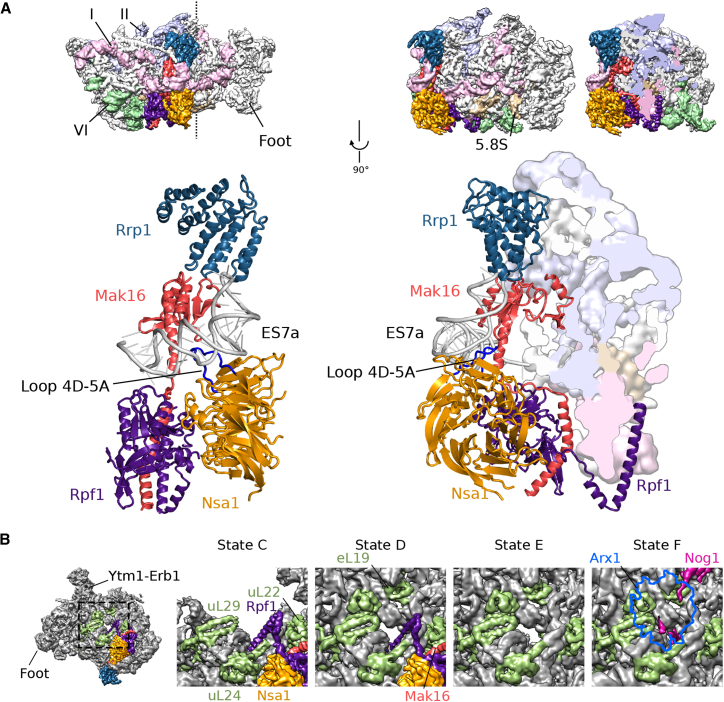
Nsa1 Module and Formation of the PET (A) Binding site of the Nsa1 module consisting of Mak16 (red), Nsa1 (orange), Rpf1 (purple), and Rrp1 (dark blue) bound to ES7a (light gray). A back and side view ...
Figureu00a03
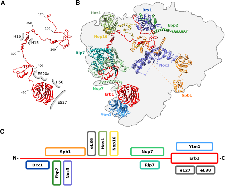
Erb1 Functions as a Multivalent Interaction Hub (A) Overview of the Erb1 domain architectureu00a0showing the extended N terminus and theu00a0doughnut-shaped WD40 repeat domain. Interactions with rRNA ...
Figureu00a04
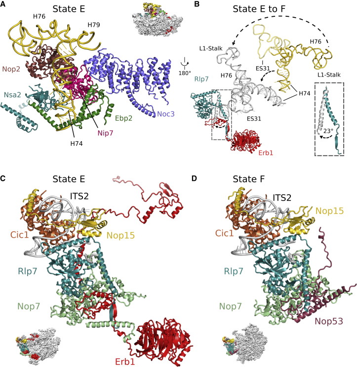
Maturation of the L1-Stalk Segment Is Linked to u201cFootu201d Remodeling (A) The L1 segment (rRNA helices H74u2013H79, gold) is stabilized in a pre-mature conformation by a set of AFs, including Ebp2...
Figureu00a05
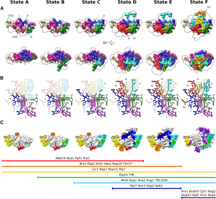
Sequential Incorporation of the rRNA Domains into a Developing Pre-60S Core Particle (A) Front and top views of structural rRNA representations based on Chimera molmaps for states Au2013F. The molmaps...
Figureu00a06
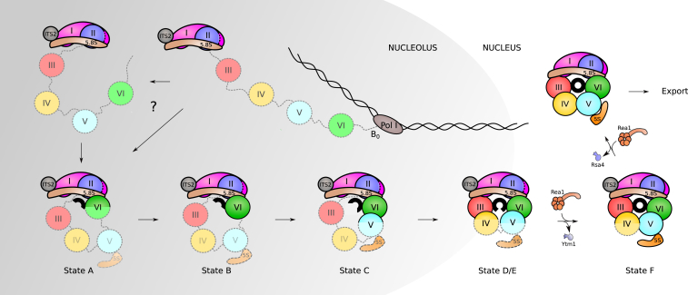
Assembly Sequence of the Pre-rRNA Domains Assembly of RPs and AFs to the nascent 35S rRNA precursor starts co-transcriptionally. Very early, the pre-rRNA is circularized as domain VI binds to domains ...
Figure images are served from the NIH/NLM PubMed Central Open Access Subset or Europe PMC; copyright remains with the publishers and authors.
💬 Discussion
0 commentsNo comments yet. Be the first to start a discussion!
Leave a Comment