Abstract
To image the accessible genome at nanometer scale in situ, we developed three-dimensional assay for transposase-accessible chromatin-photoactivated localization microscopy (3D ATAC-PALM) that integrates an assay for transposase-accessible chromatin with visualization, PALM super-resolution imaging and lattice light-sheet microscopy. Multiplexed with oligopaint DNA-fluorescence in situ hybridization (FISH), RNA-FISH and protein fluorescence, 3D ATAC-PALM connected microscopy and genomic data, revealing spatially segregated accessible chromatin domains (ACDs) that enclose active chromatin and transcribed genes. Using these methods to analyze genetically perturbed cells, we demonstrated that genome architectural protein CTCF prevents excessive clustering of accessible chromatin and decompacts ACDs. These results highlight 3D ATAC-PALM as a useful tool to probe the structure and organizing mechanism of the genome.
🔬 Techniques
🧬 Organisms
💻 Software
✨ Fluorophores
🧪 Sample Preparation
🔬 Cell Lines
🏭 Microscope Brands
🧪 Reagent Suppliers
📷 Detectors
💻 Software Details
💾 Data Repositories
🏛️ Research Organizations (ROR)
Affiliated research institutions:
📋 Methods
Tn5 Expression and Purification
The plasmid pTXB1-Tn5 (Addgene #60240) was used to express the hyperactive Tn5 transposase fused with the Mxe Intein and Chitin-binding domain 45 . Briefly, the pTXB1-Tn5 was transformed into the T7 Express lysY/Iq Competent E. coli (NEB, cat# C3013I). 1 litter culture of transformed cells were grown in TB buffer with antibiotics at 37°C to A 600 ~0.6 and induced with 0.25 mM IPTG. The cells were incubated at 23°C for 4 h, harvested, and washed with 50 mL 1× PBS with cOmplete™ Protease Inhibitor Cocktail (Roche). The cell pellet was snap frozen in liquid nitrogen, stored at −80°C overnight, resuspended in 160 mL HEGX (20 mM HEPES-KOH at pH 7.2, 0.8 M NaCl, 1 mM EDTA, 10% glycerol, 0.2% Triton X-100) with Protease Inhibitor and sonicated for 10 cycles of 30s ON/60s OFF at 30 W output on a Model 100 Sonic Dismembrator (Fisher Scientific). The lysate was centrifuged in a Beckman JA25.50 rotor at 16,000 rpm for 30 min at 4°C and 8.4 mL 5% neutralized PEI (Sigma P3143) was added dropwise into the supernatant with gentle agitation for 15 minutes at 4°C followed by another centrifuge at 13,000 rpm for 10 min at 4°C. Meantime 20 mL Chitin Resin (NEB cat#S6651L) was equilibrated in a column with 200mL of HEGX buffer supplemented with protease inhibitor and loaded with the supernatant from the PEI-centrifuge step by slow gravity flow (12 hours) with constant stirring and protection from light. The conjugation reaction was further precipitated by 3M sodium acetate, pH 5.2 and ethanol. The purified pellet was dissolved in 0.1 M TEAA (triethylammonium acetate) (Thermo Fisher Scientific cat# 400613). Purification of oligo-dye conjugates were performed on Agilent 1200 Analytical HPLC system equipped with an autosampler, diode array detector and fraction collector. The column used was Eclipse XDB-C18 column (4.6 × 150 mm 5 μm, Agilent) and eluted with a linear gradient of 0–100% MeCN/H 2 O with constant 10 mM TEAA additive; 30 min run; 1ml/min flow, detection at 260 nm. Sample fractions were pooled and lyophilized to obtain the product as white solid. In vitro Tn5 transposome assembly, validation and preparation for PALM imaging The HPLC purified Tn5ME-A-PA-JF 549 , Tn5ME-B-PA-JF 549 , Tn5MErev oligos were resuspended in water to 100 μM each. Tn5ME-A-PA-JF 549 or Tn5ME-B-PA-JF 549 were mixed with Tn5MERev in each molar ratio in 1X annealing buffer (10mM Tris HCl pH8.0, 50mM NaCl, 1mM EDTA) and were denatured on a benchtop thermocycler at 95 °C for 5 min and then slowly cooled down to 25°C at the rate of −1°C /min. We assembled the Tn5 transposome with PA-JF 549 according to previously published protocol 12 by combining 0.25 vol Tn5MErev/Tn5ME-A-PA-JF 549 + Tn5MErev/Tn5ME-B-PA- JF 549 (50 μM each), 0.4 vol glycerol (100% solution), 0.12 vol 2× dialysis buffer (100 mM HEPES–KOH at pH 7.2, 0.2 M NaCl, 0.2 mM EDTA, 2 mM DTT, 0.2% Triton X-100, 20% glycerol), 0.1 vol Tn5 (50 μM), 0.13 vol H2O, followed by gentle nutation at room temperature for 1 hour. The activity of in-house prepared Tn5 transposome was validated by genome-wide ATAC-seq as described previously 12 following an reverse crosslinking step. We prepared cells for 3D ATAC-PALM experiments as reported previously 12 . Briefly, cells (mouse ESC or MEF) were plated onto #1 thickness 5mm coverslips (Warner Instruments, cat#64–0700) at around 70–80% confluency with proper coating one day before experiment. Cells were fixed with 1% paraformaldehyde (Electron Microscopy Sciences, Cat# 15710) for 10 min at room temperature. After fixation, cells were washed three times with 1 X PBS for 5 minutes and then permeabilized with ATAC lysis buffer (10 mM Tris–Cl, pH 7.4, 10 mM NaCl, 3 mM MgCl2, 0.1% Igepal CA-630) for 10 min at room temperature. After permeabilization, the slides were washed twice in 1XPBS and put inside a humidity chamber box at 37 °C. The transposase mixture solution (1× Tagmentation buffer-10mM Tris-HCl, pH 7.6, 5mM MgCl2, 10% dimethylformamide, 100 nM Tn5- PA-JF 549 ) was added to the cells and incubated for 30 min at 37 °C inside the humidity chamber. After the transposase reaction, slides were washed three times with 1 X PBS containing 0.01% SDS and 50 mM EDTA for 15 min at 55 °C before mounted onto the Lattice light-sheet microscope (LLSM) slot for 3D ATAC-PALM imaging. 3D ATAC-PALM image acquisition and processing The 3D ATAC-PALM data were acquired by the Lattice light-sheet microscopy 15 at room temperature. The light sheet was generated from the interference of highly parallel beams in a square lattice and dithered to create a uniform excitation sheet. The inner and outer numerical apertures of the excitation sheet were set to be 0.44 and 0.55, respectively. A Variable-Flow Peristaltic Pump (Thermo Fisher Scientific) was used to connect a 2L reservoir with the imaging chamber with 1×PBS circulating through at a constant flow rate. Labelled cells seeded on 5mm coverslips (Warner Instruments) were placed into the imaging chamber and each image volume includes ~100–200 image frames, depending on the depth of field of view. Specifically, spontaneously activated PA-JF 549 dye were initially pushed into the fluorescent dark state through repeated photo-bleaching by scanning the whole image view with a 2W 560 nm laser (MPB Communications Inc., Canada). Then, the samples were imaged by iteratively photo-activating each plane with very low intensity 405 nm light (95%) of localizations fall into the nuclear H2B mask, suggesting that the manual segmentation based on ATAC-PALM signal intensity is sufficient to distinguish it from out-of-nucleus signal (e.g. mitochondria) or non-specific background. To derive the ATAC-PALM intensity map in order to compare with HP1-GFP labeled heterochromatin spatial distribution, ATAC-PALM localizations were binned within a cubic of 100 nm with a 3D Gaussian filter and a convolution kernel of 3×3×3. 3D pair auto-correlation function, pair cross-correlation function and Ripley’s function As described previously 46 , the pair correlation function g 0 ( r ) or radial distribution function measures the probability P of finding a localization of accessible chromatin in a volume element dV at a separation r from another accessible chromatin site: (Equation S5) P = ρ ⋅ g 0 ( r ) ⋅ d V Where ρ represents the mean density of accessible chromatin in the nucleus. 3D g 0 ( r ) was computed by (Equation S6) g 0 ( r ) = 3 V 4 π ( 3 r 2 ⋅ Δ r + 3 r ⋅ Δ r 2 + Δ r 3 ) ⋅ 1 N ⋅ ( N − 1 ) ∑ i = 1 N ∑ i ≠ j δ ( r − r i j ) N is the total number of localizations and V is the 3D nuclear volume. Δ r = 50 nm is the binning width used in the analysis. The item 4 π (3 r 2 ·Δ r + 3 r ·Δ r 2 + Δ r 3 )/3 represents the shell-shape volume between the search radius from r to r + Δ r . The Dirac Delta function is defined by (Equation S7) δ ( r − r i j ) = { 1 r − r i j ≤ Δ r 0 r − r i j > Δ r Where r ij represents the pair-wise Euclidean distance between localization point i and j . To eliminate the boundary effect in calculation of g 0 ( r ) from a finite 3D volume, we generated g r ( r ) from uniform distributions with the same localization density in the same volume as real data using the Matlab convex hull function. Accordingly, the final normalized 3D pair auto-correlation function G ( r ) was calculated by: (Equation S8) G ( r ) = g 0 ( r ) g r ( r ) Similarly, the 3D pair cross-correlation function c 0 ( r ) between localizations of molecule A and those of molecule B can be formulated as (Equation S9) c 0 ( r ) = 3 V 4 π ( 3 r 2 ⋅ Δ r + 3 r ⋅ Δ r 2 + Δ r 3 ) ⋅ 1 M ⋅ N ∑ i = 1 M ∑ j = 1 N δ ( r − r i j ) M is the total number of localizations for molecule A and N is the total number of localizations for molecule B. The Dirac Delta function is defined as the same as in Equation S7 . Similarly, the final normalized 3D pair auto-correlation function C ( r ) was calculated by: (Equation S10) C ( r ) = c 0 ( r ) c r ( r ) c r ( r ) refers to the pair cross-correlation function calculated from uniform distributions with the same localization density in the same volume as real data used. Ripley’s K function is a variation of pair correlation function to study point distribution patterns and is defined by the equation: (Equation S11) K ( r ) = V N − 1 [ 1 N ∑ i = 1 N ∑ i ≠ j δ K ( r − r i j ) ] where its Delta function given by δ K ( r − r i j ) = { 1 r − r i j ≤ 0 0 r − r i j > 0 The K ( r ) for a random Poisson distribution is πr 2 . Therefore, its derivative Ripley’s L function is given by (Equation S12) L ( r ) = K ( r ) π The deviation of L ( r ) from expected random Poisson distribution can be used to indicate point clustering or dispersion. The further normalized Ripley’s H function (Equation S13) H ( r ) = L ( r ) − r Can be used to estimate the point clustering and domain size 47 . Whereas G ( r ) can be used as bona fide criteria for estimating the clustering effect of a group of spatial localizations, it has to be adjusted regarding the inevitable localization uncertainty of the PSF. If the distribution is purely random, the revised pair auto-correlation G R ( r ) considering PSF uncertainty is given by (Equation S14) G R ( r ) = G P S F ( r ) + 1 with (Equation S15) G P S F ( r ) = 1 8 π 3 / 2 σ 3 e − r 2 / 4 σ 2 where ρ represents the average surface density of molecules, G PSF ( r ) denotes the correlation of uncertainty in the PSF and σ for standard deviation. The spatial autocorrelation of accessible chromatin can be approximated by an exponential function: (Equation S16) g ( r ) = A ⋅ e − r / ε + 1 where ε and A denotes the correlation length and amplitude of the accessible chromatin cluster, respectively. The total correlation can be described by (Equation S17) G ( r ) = G P S F ( r ) + ( A ⋅ e − r / ε + 1 ) ⊗ G P S F ( r ) The raw data were fitted by using Equation S17 to derive g ( r ) and parameters A and ε . The approximated function g ( r ) was used throughout the paper for pair auto-correlation analysis. Curve fitting was performed using the trust-region method implemented in the Curve Fitting Matlab toolbox. Since over-counting does not give rise to apparent co-clustering in double label experiments when pair cross-correlation functions are measured 48 , C ( r ) can serve as bona fide criteria for estimating the co-clustering effect of spatial localizations from two different channels without additional adjustment. 2D pair cross-correlation function and auto-correlation function To calculate the spatial cross-correlation between the two-color ATAC localization signal and the heterochromatin HP1α signal, we first converted the localization densities into intensity map via 2D Gaussian blurring. The pair cross-correlation function c ( r → ) was then calculated by the fast Fourier transform (FFT) method described previously 46 . (Equation S18) c ( r → ) = Re { F F T − 1 ( F F T ( I 1 ) × conj [ F F T ( I 2 ) ] ) ρ 1 ρ 2 N ( r → ) } (Equation S19) N ( r → ) = F F T − 1 ( | F F T ( Mask ) | 2 ) The N ( r → ) is the auto-correlation of a mask matrix that has the value of 1 inside the nucleus used for normalization. Conj [] refers to complex conjugate, ρ 1 and ρ 2 are the average surface densities (number of localizations divided by the surface area) of images I 1 and I 2 , and Re{} indicates the real part. The fast Fourier transform and its inverse ( FFT and FFT −1 ) were computed by fft2() and ifft2() functions in Matlab, respectively. Cross correlation functions were calculated first by converting the Cartesian coordinates to polar coordinates by Matlab cart2pol() function, binning by radius and by averaging within the assigned bins.
Show full methods section
Tn5 Expression and Purification
The plasmid pTXB1-Tn5 (Addgene #60240) was used to express the hyperactive Tn5 transposase fused with the Mxe Intein and Chitin-binding domain 45 . Briefly, the pTXB1-Tn5 was transformed into the T7 Express lysY/Iq Competent E. coli (NEB, cat# C3013I). 1 litter culture of transformed cells were grown in TB buffer with antibiotics at 37°C to A 600 ~0.6 and induced with 0.25 mM IPTG. The cells were incubated at 23°C for 4 h, harvested, and washed with 50 mL 1× PBS with cOmplete™ Protease Inhibitor Cocktail (Roche). The cell pellet was snap frozen in liquid nitrogen, stored at −80°C overnight, resuspended in 160 mL HEGX (20 mM HEPES-KOH at pH 7.2, 0.8 M NaCl, 1 mM EDTA, 10% glycerol, 0.2% Triton X-100) with Protease Inhibitor and sonicated for 10 cycles of 30s ON/60s OFF at 30 W output on a Model 100 Sonic Dismembrator (Fisher Scientific). The lysate was centrifuged in a Beckman JA25.50 rotor at 16,000 rpm for 30 min at 4°C and 8.4 mL 5% neutralized PEI (Sigma P3143) was added dropwise into the supernatant with gentle agitation for 15 minutes at 4°C followed by another centrifuge at 13,000 rpm for 10 min at 4°C. Meantime 20 mL Chitin Resin (NEB cat#S6651L) was equilibrated in a column with 200mL of HEGX buffer supplemented with protease inhibitor and loaded with the supernatant from the PEI-centrifuge step by slow gravity flow (12 hours) with constant stirring and protection from light. The conjugation reaction was further precipitated by 3M sodium acetate, pH 5.2 and ethanol. The purified pellet was dissolved in 0.1 M TEAA (triethylammonium acetate) (Thermo Fisher Scientific cat# 400613). Purification of oligo-dye conjugates were performed on Agilent 1200 Analytical HPLC system equipped with an autosampler, diode array detector and fraction collector. The column used was Eclipse XDB-C18 column (4.6 × 150 mm 5 μm, Agilent) and eluted with a linear gradient of 0–100% MeCN/H 2 O with constant 10 mM TEAA additive; 30 min run; 1ml/min flow, detection at 260 nm. Sample fractions were pooled and lyophilized to obtain the product as white solid. In vitro Tn5 transposome assembly, validation and preparation for PALM imaging The HPLC purified Tn5ME-A-PA-JF 549 , Tn5ME-B-PA-JF 549 , Tn5MErev oligos were resuspended in water to 100 μM each. Tn5ME-A-PA-JF 549 or Tn5ME-B-PA-JF 549 were mixed with Tn5MERev in each molar ratio in 1X annealing buffer (10mM Tris HCl pH8.0, 50mM NaCl, 1mM EDTA) and were denatured on a benchtop thermocycler at 95 °C for 5 min and then slowly cooled down to 25°C at the rate of −1°C /min. We assembled the Tn5 transposome with PA-JF 549 according to previously published protocol 12 by combining 0.25 vol Tn5MErev/Tn5ME-A-PA-JF 549 + Tn5MErev/Tn5ME-B-PA- JF 549 (50 μM each), 0.4 vol glycerol (100% solution), 0.12 vol 2× dialysis buffer (100 mM HEPES–KOH at pH 7.2, 0.2 M NaCl, 0.2 mM EDTA, 2 mM DTT, 0.2% Triton X-100, 20% glycerol), 0.1 vol Tn5 (50 μM), 0.13 vol H2O, followed by gentle nutation at room temperature for 1 hour. The activity of in-house prepared Tn5 transposome was validated by genome-wide ATAC-seq as described previously 12 following an reverse crosslinking step. We prepared cells for 3D ATAC-PALM experiments as reported previously 12 . Briefly, cells (mouse ESC or MEF) were plated onto #1 thickness 5mm coverslips (Warner Instruments, cat#64–0700) at around 70–80% confluency with proper coating one day before experiment. Cells were fixed with 1% paraformaldehyde (Electron Microscopy Sciences, Cat# 15710) for 10 min at room temperature. After fixation, cells were washed three times with 1 X PBS for 5 minutes and then permeabilized with ATAC lysis buffer (10 mM Tris–Cl, pH 7.4, 10 mM NaCl, 3 mM MgCl2, 0.1% Igepal CA-630) for 10 min at room temperature. After permeabilization, the slides were washed twice in 1XPBS and put inside a humidity chamber box at 37 °C. The transposase mixture solution (1× Tagmentation buffer-10mM Tris-HCl, pH 7.6, 5mM MgCl2, 10% dimethylformamide, 100 nM Tn5- PA-JF 549 ) was added to the cells and incubated for 30 min at 37 °C inside the humidity chamber. After the transposase reaction, slides were washed three times with 1 X PBS containing 0.01% SDS and 50 mM EDTA for 15 min at 55 °C before mounted onto the Lattice light-sheet microscope (LLSM) slot for 3D ATAC-PALM imaging. 3D ATAC-PALM image acquisition and processing The 3D ATAC-PALM data were acquired by the Lattice light-sheet microscopy 15 at room temperature. The light sheet was generated from the interference of highly parallel beams in a square lattice and dithered to create a uniform excitation sheet. The inner and outer numerical apertures of the excitation sheet were set to be 0.44 and 0.55, respectively. A Variable-Flow Peristaltic Pump (Thermo Fisher Scientific) was used to connect a 2L reservoir with the imaging chamber with 1×PBS circulating through at a constant flow rate. Labelled cells seeded on 5mm coverslips (Warner Instruments) were placed into the imaging chamber and each image volume includes ~100–200 image frames, depending on the depth of field of view. Specifically, spontaneously activated PA-JF 549 dye were initially pushed into the fluorescent dark state through repeated photo-bleaching by scanning the whole image view with a 2W 560 nm laser (MPB Communications Inc., Canada). Then, the samples were imaged by iteratively photo-activating each plane with very low intensity 405 nm light (95%) of localizations fall into the nuclear H2B mask, suggesting that the manual segmentation based on ATAC-PALM signal intensity is sufficient to distinguish it from out-of-nucleus signal (e.g. mitochondria) or non-specific background. To derive the ATAC-PALM intensity map in order to compare with HP1-GFP labeled heterochromatin spatial distribution, ATAC-PALM localizations were binned within a cubic of 100 nm with a 3D Gaussian filter and a convolution kernel of 3×3×3. 3D pair auto-correlation function, pair cross-correlation function and Ripley’s function As described previously 46 , the pair correlation function g 0 ( r ) or radial distribution function measures the probability P of finding a localization of accessible chromatin in a volume element dV at a separation r from another accessible chromatin site: (Equation S5) P = ρ ⋅ g 0 ( r ) ⋅ d V Where ρ represents the mean density of accessible chromatin in the nucleus. 3D g 0 ( r ) was computed by (Equation S6) g 0 ( r ) = 3 V 4 π ( 3 r 2 ⋅ Δ r + 3 r ⋅ Δ r 2 + Δ r 3 ) ⋅ 1 N ⋅ ( N − 1 ) ∑ i = 1 N ∑ i ≠ j δ ( r − r i j ) N is the total number of localizations and V is the 3D nuclear volume. Δ r = 50 nm is the binning width used in the analysis. The item 4 π (3 r 2 ·Δ r + 3 r ·Δ r 2 + Δ r 3 )/3 represents the shell-shape volume between the search radius from r to r + Δ r . The Dirac Delta function is defined by (Equation S7) δ ( r − r i j ) = { 1 r − r i j ≤ Δ r 0 r − r i j > Δ r Where r ij represents the pair-wise Euclidean distance between localization point i and j . To eliminate the boundary effect in calculation of g 0 ( r ) from a finite 3D volume, we generated g r ( r ) from uniform distributions with the same localization density in the same volume as real data using the Matlab convex hull function. Accordingly, the final normalized 3D pair auto-correlation function G ( r ) was calculated by: (Equation S8) G ( r ) = g 0 ( r ) g r ( r ) Similarly, the 3D pair cross-correlation function c 0 ( r ) between localizations of molecule A and those of molecule B can be formulated as (Equation S9) c 0 ( r ) = 3 V 4 π ( 3 r 2 ⋅ Δ r + 3 r ⋅ Δ r 2 + Δ r 3 ) ⋅ 1 M ⋅ N ∑ i = 1 M ∑ j = 1 N δ ( r − r i j ) M is the total number of localizations for molecule A and N is the total number of localizations for molecule B. The Dirac Delta function is defined as the same as in Equation S7 . Similarly, the final normalized 3D pair auto-correlation function C ( r ) was calculated by: (Equation S10) C ( r ) = c 0 ( r ) c r ( r ) c r ( r ) refers to the pair cross-correlation function calculated from uniform distributions with the same localization density in the same volume as real data used. Ripley’s K function is a variation of pair correlation function to study point distribution patterns and is defined by the equation: (Equation S11) K ( r ) = V N − 1 [ 1 N ∑ i = 1 N ∑ i ≠ j δ K ( r − r i j ) ] where its Delta function given by δ K ( r − r i j ) = { 1 r − r i j ≤ 0 0 r − r i j > 0 The K ( r ) for a random Poisson distribution is πr 2 . Therefore, its derivative Ripley’s L function is given by (Equation S12) L ( r ) = K ( r ) π The deviation of L ( r ) from expected random Poisson distribution can be used to indicate point clustering or dispersion. The further normalized Ripley’s H function (Equation S13) H ( r ) = L ( r ) − r Can be used to estimate the point clustering and domain size 47 . Whereas G ( r ) can be used as bona fide criteria for estimating the clustering effect of a group of spatial localizations, it has to be adjusted regarding the inevitable localization uncertainty of the PSF. If the distribution is purely random, the revised pair auto-correlation G R ( r ) considering PSF uncertainty is given by (Equation S14) G R ( r ) = G P S F ( r ) + 1 with (Equation S15) G P S F ( r ) = 1 8 π 3 / 2 σ 3 e − r 2 / 4 σ 2 where ρ represents the average surface density of molecules, G PSF ( r ) denotes the correlation of uncertainty in the PSF and σ for standard deviation. The spatial autocorrelation of accessible chromatin can be approximated by an exponential function: (Equation S16) g ( r ) = A ⋅ e − r / ε + 1 where ε and A denotes the correlation length and amplitude of the accessible chromatin cluster, respectively. The total correlation can be described by (Equation S17) G ( r ) = G P S F ( r ) + ( A ⋅ e − r / ε + 1 ) ⊗ G P S F ( r ) The raw data were fitted by using Equation S17 to derive g ( r ) and parameters A and ε . The approximated function g ( r ) was used throughout the paper for pair auto-correlation analysis. Curve fitting was performed using the trust-region method implemented in the Curve Fitting Matlab toolbox. Since over-counting does not give rise to apparent co-clustering in double label experiments when pair cross-correlation functions are measured 48 , C ( r ) can serve as bona fide criteria for estimating the co-clustering effect of spatial localizations from two different channels without additional adjustment. 2D pair cross-correlation function and auto-correlation function To calculate the spatial cross-correlation between the two-color ATAC localization signal and the heterochromatin HP1α signal, we first converted the localization densities into intensity map via 2D Gaussian blurring. The pair cross-correlation function c ( r → ) was then calculated by the fast Fourier transform (FFT) method described previously 46 . (Equation S18) c ( r → ) = Re { F F T − 1 ( F F T ( I 1 ) × conj [ F F T ( I 2 ) ] ) ρ 1 ρ 2 N ( r → ) } (Equation S19) N ( r → ) = F F T − 1 ( | F F T ( Mask ) | 2 ) The N ( r → ) is the auto-correlation of a mask matrix that has the value of 1 inside the nucleus used for normalization. Conj [] refers to complex conjugate, ρ 1 and ρ 2 are the average surface densities (number of localizations divided by the surface area) of images I 1 and I 2 , and Re{} indicates the real part. The fast Fourier transform and its inverse ( FFT and FFT −1 ) were computed by fft2() and ifft2() functions in Matlab, respectively. Cross correlation functions were calculated first by converting the Cartesian coordinates to polar coordinates by Matlab cart2pol() function, binning by radius and by averaging within the assigned bins.
DBSCAN analysis
The density-based clustering algorithm DBSCAN (Density-Based Spatial Clustering of Applications with Noise) was adopted to map and visualize individual local ACDs (core DBSCAN Matlab code from http://yarpiz.com/255/ypml110-dbscan-clustering ). The algorithm first finds neighboring data points within a sphere of radius r , and adds them into same group. In parallel, a predefined threshold minimal points ( minPts ) was used by the algorithm to justify whether any counted group is a cluster. If the number of points within a group is less than the threshold minPts , the data point is classified as noise. As a negative control, we generated uniformly sampled data sets with the same localization density as our ATAC-PALM localizations. We then implemented DBSCAN analysis by using 150 nm as the searching radius ( r ) (peak radius from the Ripley’s H function analysis) and empirically setting minPts as 10. To reconstruct the iso -surface for each identified ACD, the convex hull which contains the ACD data points was calculated and visualized by using Matlab. The volume of the convex hull was computed, and the normalized cluster radius (calculated from a sphere with equal volume) was estimated and shown in violin plot. Additional methods involved in this study are included in the Supplementary Note .
Statistical Analysis
Statistical analysis was performed using Origin and GraphPad Prism. Unless stated specifically, data are presented as Mean ± SEM (standard error) with statistical significance (* p < 0.05, ** p < 0.01, *** p
📊 Figures
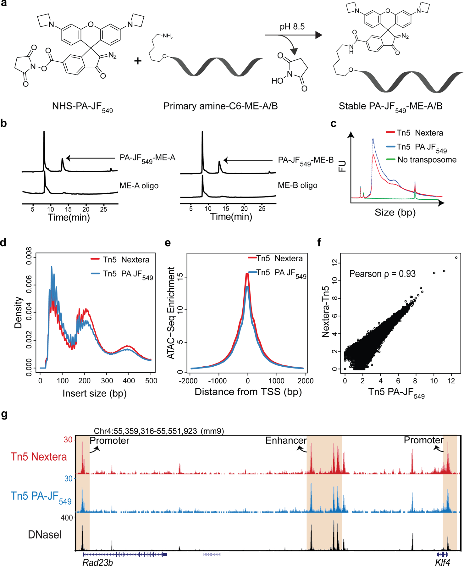
Extended Data Figure 1 |
3D ATAC-PALM labeling strategy
a , N-hydroxysuccinimide (NHS) ester chemical conjugation chemistry. PA-JF 549 dye coupled with the NHS ester reacts with the primary amine group on the Tn5 ME oligos to yield the stable dye-oligo con...
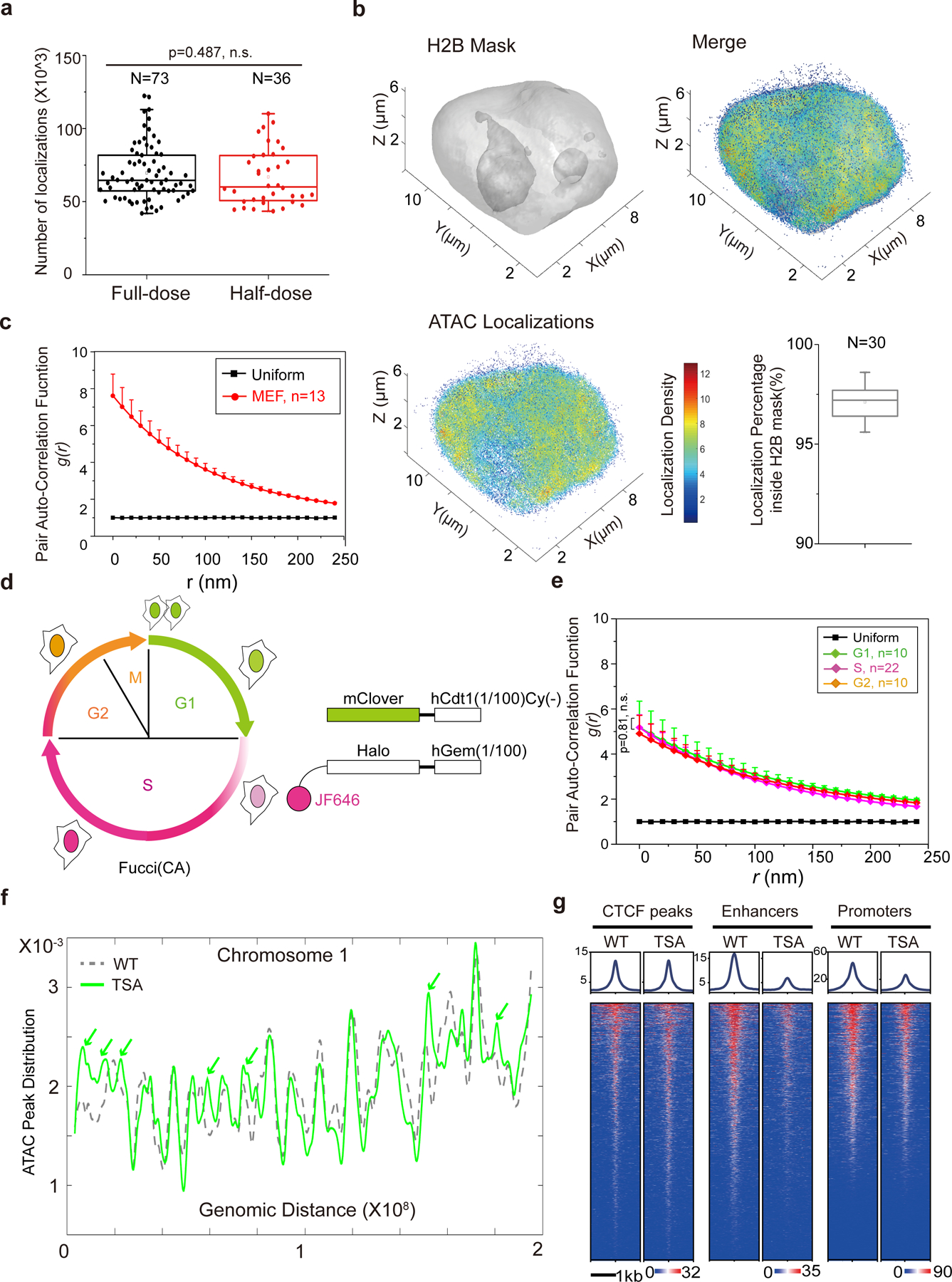
Extended Data Figure 2 |
Characterization of 3D ATAC-PALM localizations
a , The box plot compares the number of 3D ATAC-PALM localizations in the full-dose (73 cells, ~100 nM Tn5 PA-JF 549 ) and half-dose (36 cells, ~50 nM) labeling conditions. The middle line represents ...
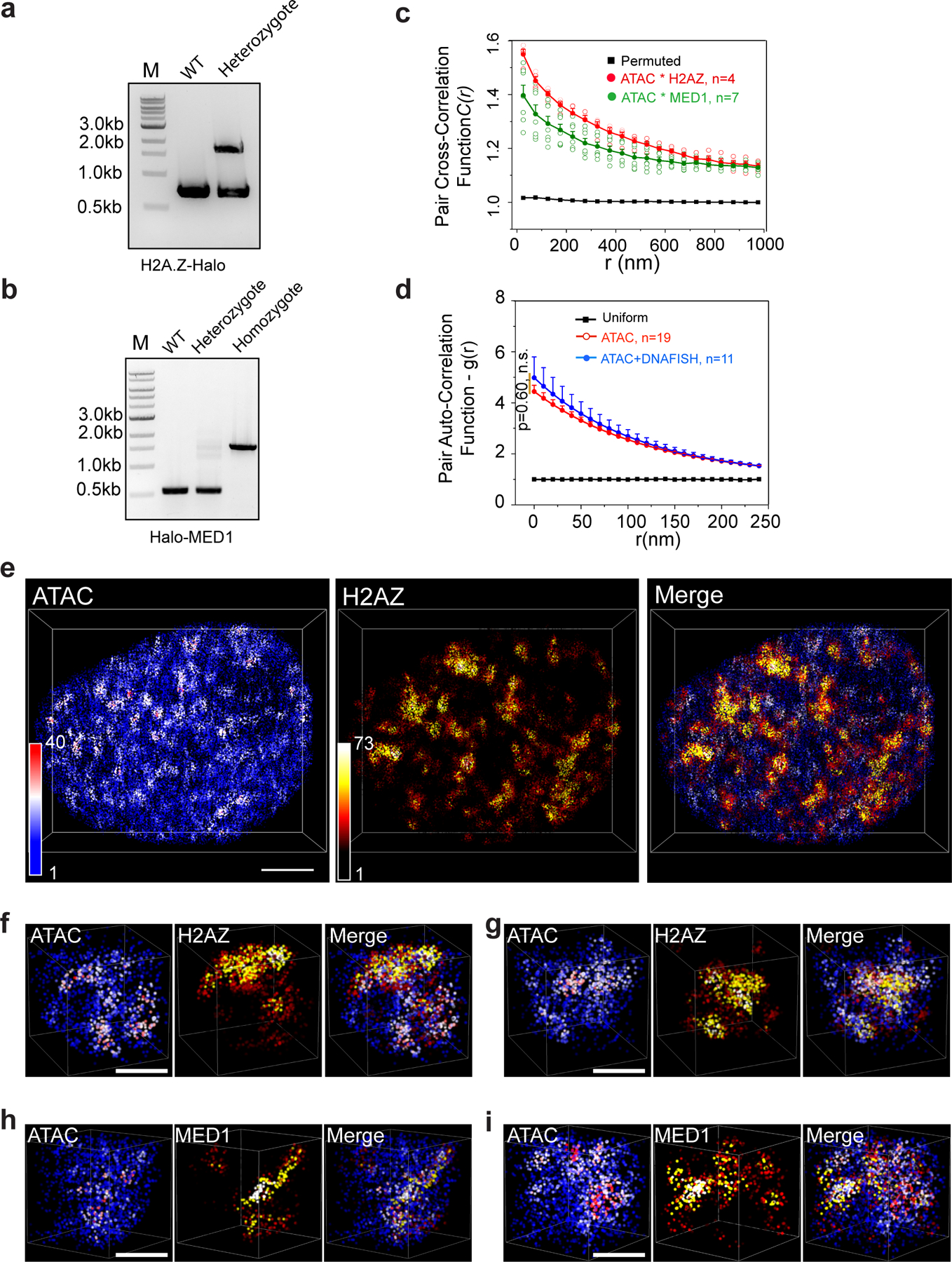
Extended Data Figure 3 |
Two-color 3D PALM imaging of accessible chromatin and landmark proteins in the active chromatin
a and b , PCR genotyping validates the correct knock-in of HaloTag in frame with histone variant H2A.Z ( a ) or Mediator subunit MED1 ( b ) coding sequence in mESCs. We obtained heterozygous and homoz...
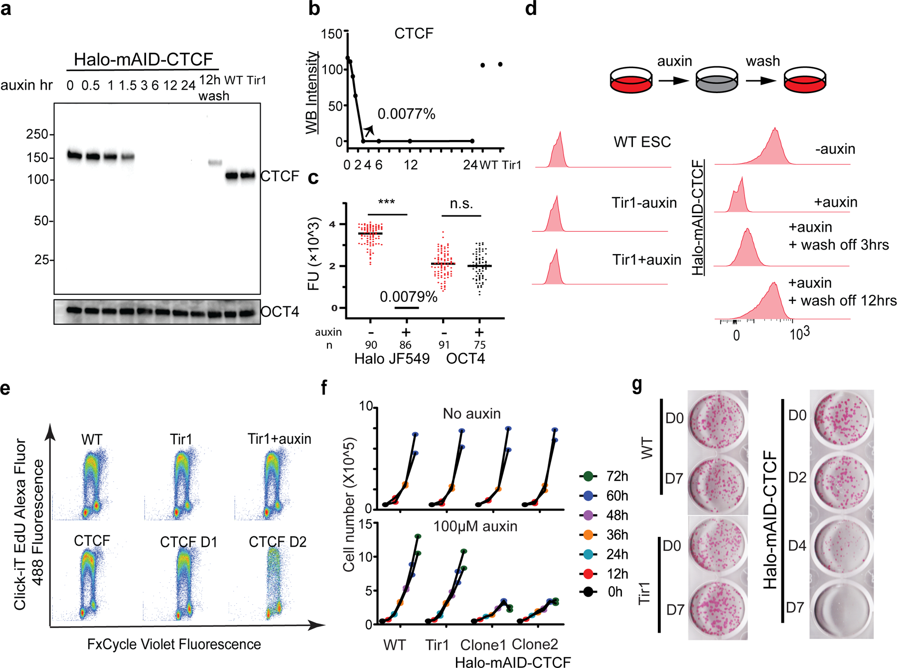
Extended Data Figure 4 |
Efficient depletion of CTCF by the AID degron system.
a , Western blotting (WB) analysis of endogenous HaloTag-mAID-CTCF at indicated time points after the auxin treatment and wash off recovery with OCT4 as the internal control. b , Quantifying WB intens...
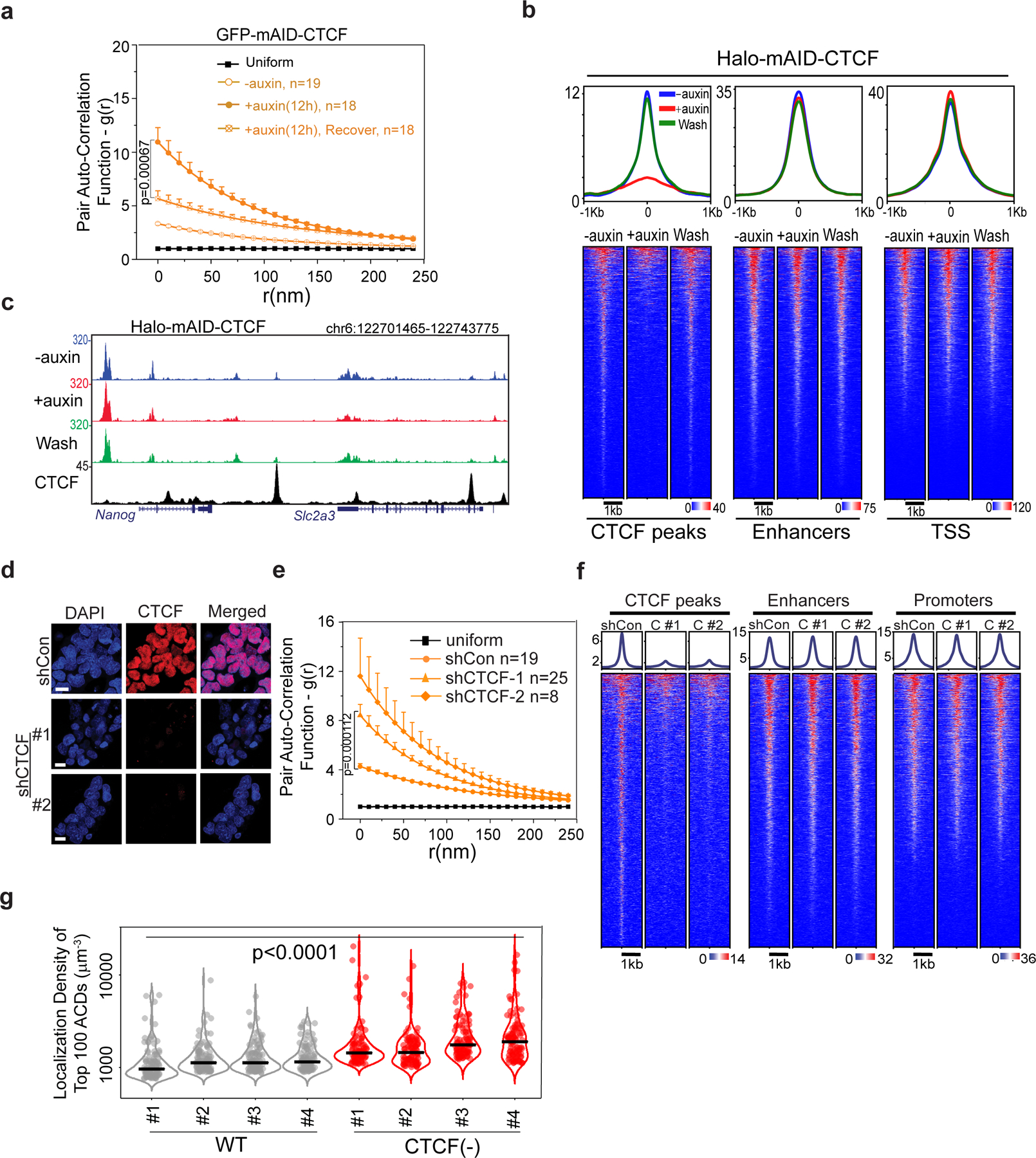
Extended Data Figure 5 |
Enhanced clustering of ACDs upon CTCF depletion.
a , Pair auto-correlation function g(r) of ATAC-PALM localizations from GFP-mAID-CTCF ESCs under normal, auxin-treated and auxin wash-off (~24 hours) conditions. The error bars represent S.E.M. Two-si...
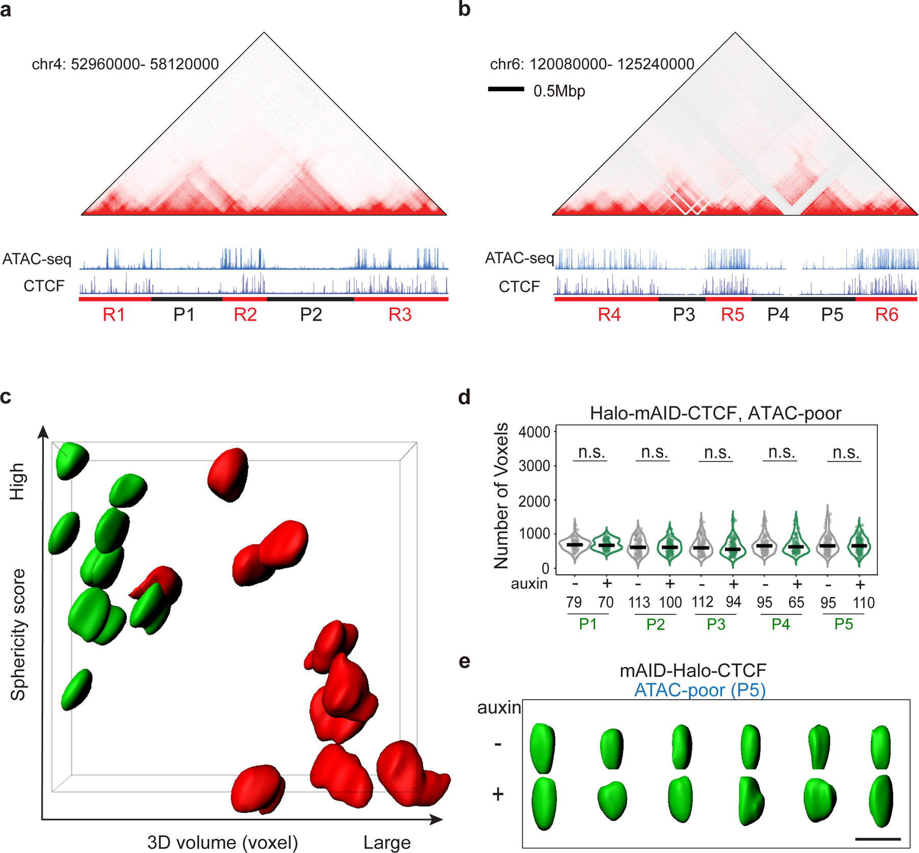
Extended Data Figure 6 |
Measuring structural changes of ATAC-rich and ATAC-poor segments upon CTCF depletion by Oligopaint DNA-FISH.
a-b , Alignment of Hi-C heatmap, ATAC-seq, CTCF ChIP-seq tracks for two chromosomal regions harboring pluripotency genes Klf4 (Chr4) and Nanog (Chr6). ATAC-rich (R1u20136; red) and ATAC-poor (P1u20135...
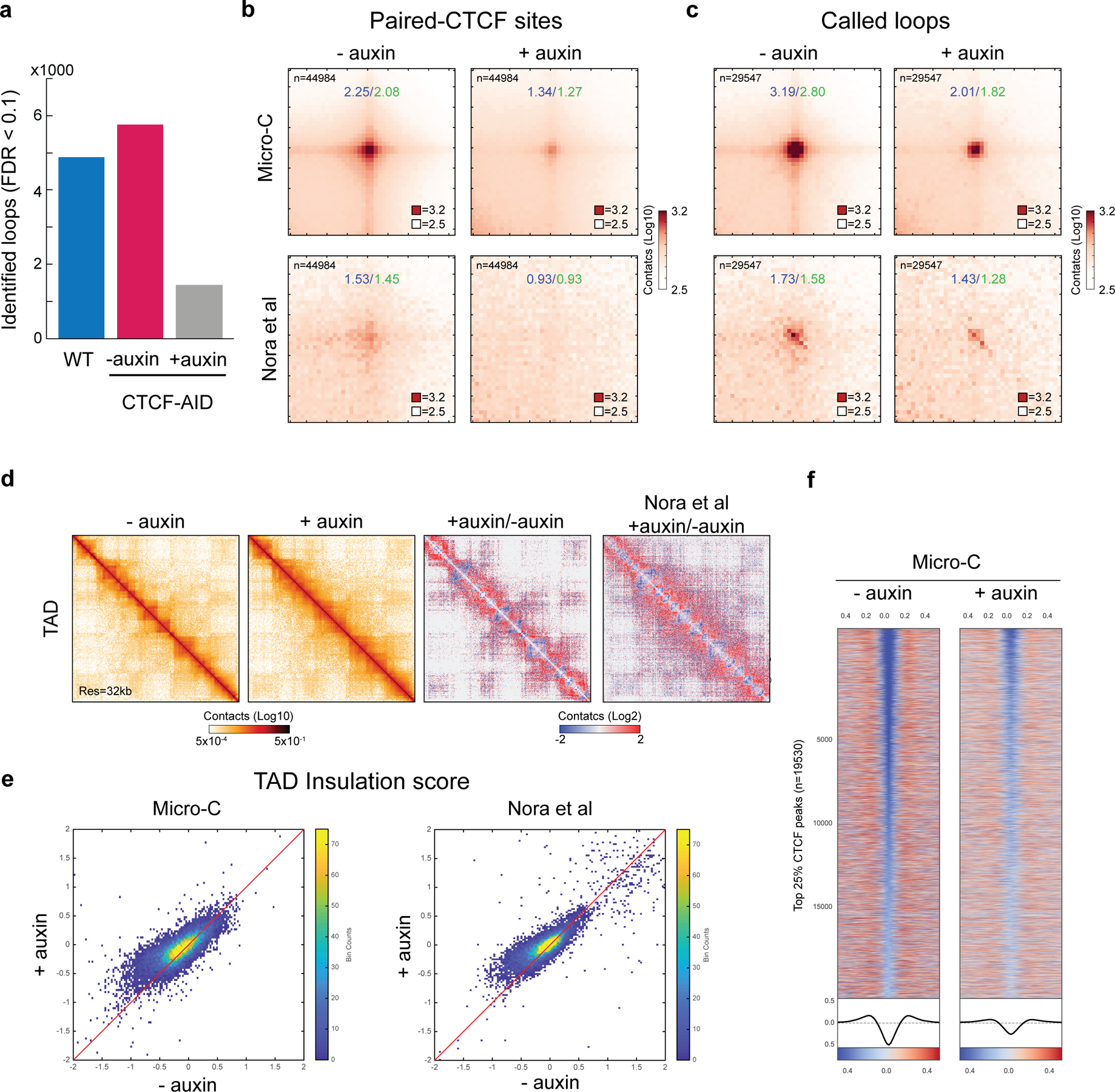
Extended Data Figure 7 |
CTCF depletion significantly reduced the number of loops and the degree of TAD domain insulation by high-resolution Micro-C analysis.
a , Number of loops in WT-mESC, CTCF-AID mESC -auxin, and +auxin conditions. We identified a similar number of loops in WT-mESC (n=4887) and CTCF-AID mESC -auxin (n=5764), while only 1442 loops were i...
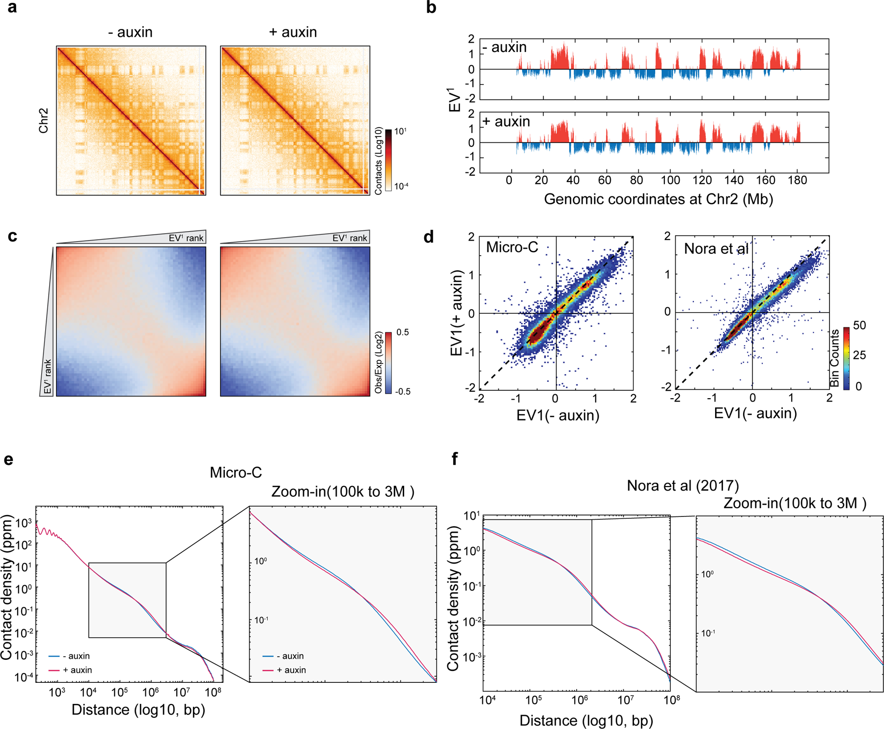
Extended Data Figure 8 |
CTCF depletion significantly increased the contact probability in A compartment by high-resolution Micro-C analysis.
a , Snapshots of Micro-C contact maps on the entire Chr2, showing the plaid-like compartments before and after auxin-mediated CTCF depletion (6 hours). b , Compartment analysis by principle component ...
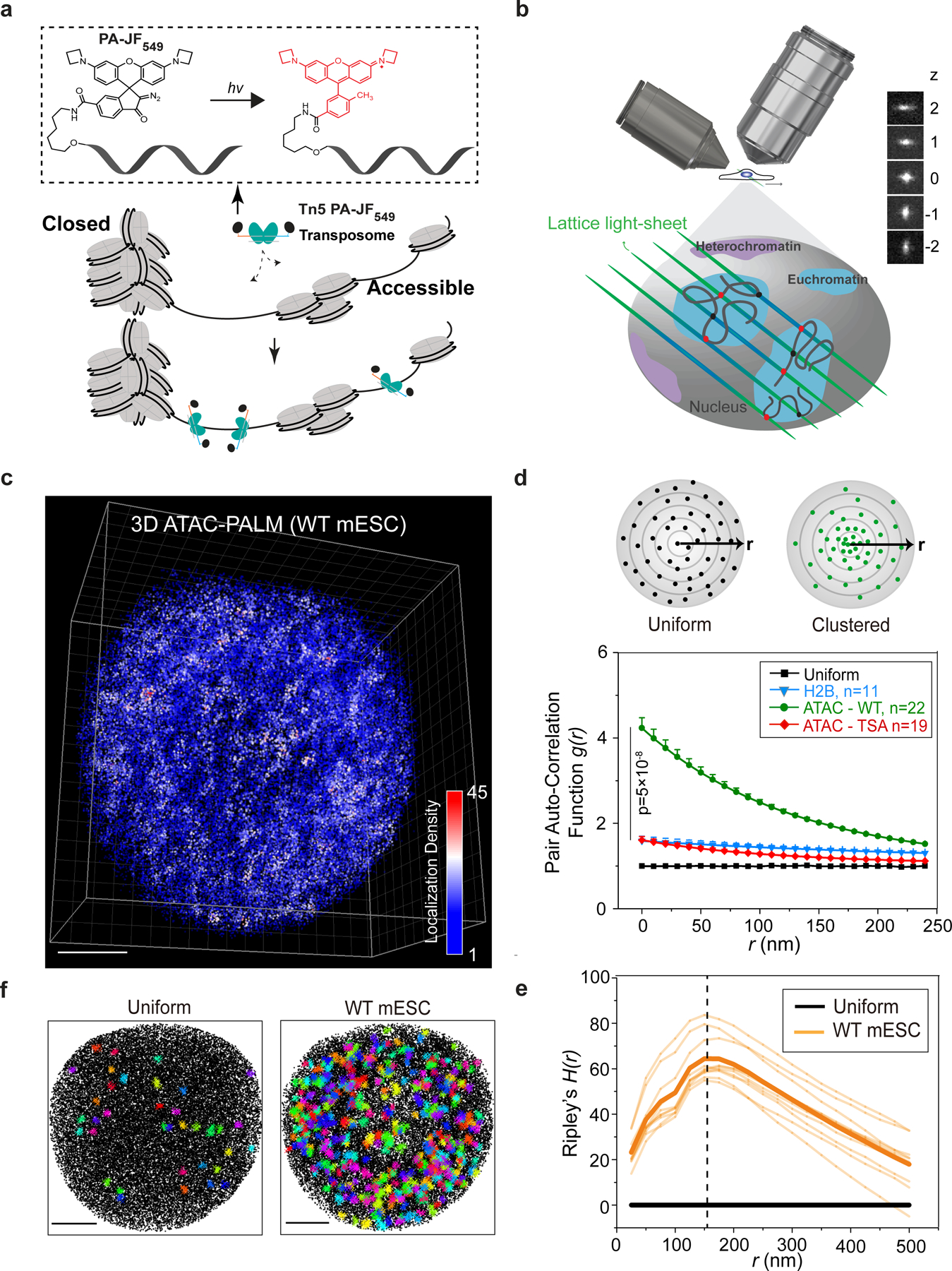
Fig. 1 |
Visualizing the accessible genome topology by 3D ATAC-PALM microscopy
a , Schematics of the 3D ATAC-PALM microscopy labeling and imaging strategy. Photoactivatable Janelia Fluor 549 (PA-JF 549 ) was conjugated to DNA oligo containing the mosaic ends of the Tn5 transposo...
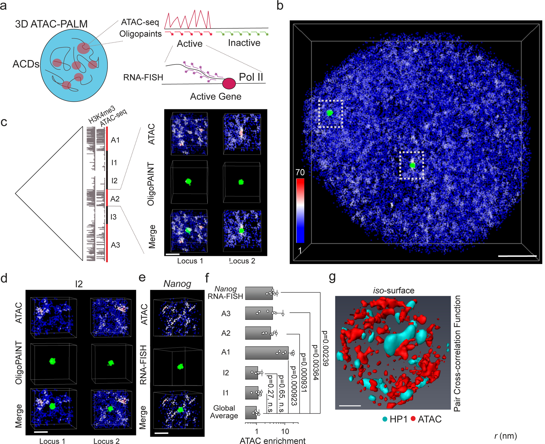
Fig. 2 |
ACDs are associated with active chromosomal segments.
a , Schematics showing multiplexed imaging of 3D ATAC-PALM and Oligopaint DNA-FISH or RNA-FISH. b , Co-localization of ACDs with ATAC-rich segments. Single-cell illustration of two color imaging of AT...
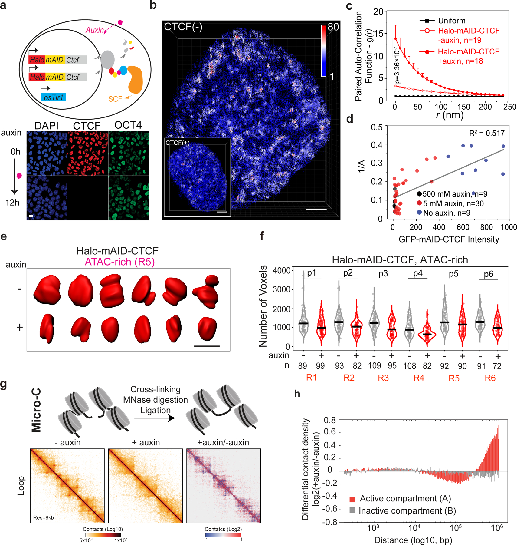
Fig. 3 |
Structural variation of accessible chromatin upon acute loss of CTCF
a , Acute depletion of CTCF in mESCs by the auxin-induced degradation system. The mini auxin-inducible degron (mAID)-HaloTag (Halo) was bi-allelically knocked into the N-terminus of Ctcf by CRISPR/Cas...
Figure images are served from the NIH/NLM PubMed Central Open Access Subset or Europe PMC; copyright remains with the publishers and authors.
💬 Discussion
0 commentsNo comments yet. Be the first to start a discussion!
Leave a Comment