Abstract
Leukocytes and other amoeboid cells change shape as they move, forming highly dynamic, actin-filled pseudopods. Although we understand much about the architecture and dynamics of thin lamellipodia made by slow-moving cells on flat surfaces, conventional light microscopy lacks the spatial and temporal resolution required to track complex pseudopods of cells moving in three dimensions. We therefore employed lattice light sheet microscopy to perform three-dimensional, time-lapse imaging of neutrophil-like HL-60 cells crawling through collagen matrices. To analyze three-dimensional pseudopods we: (i) developed fluorescent probe combinations that distinguish cortical actin from dynamic, pseudopod-forming actin networks, and (ii) adapted molecular visualization tools from structural biology to render and analyze complex cell surfaces. Surprisingly, three-dimensional pseudopods turn out to be composed of thin (<0.75 µm), flat sheets that sometimes interleave to form rosettes. Their laminar nature is not templated by an external surface, but likely reflects a linear arrangement of regulatory molecules. Although we find that Arp2/3-dependent pseudopods are dispensable for three-dimensional locomotion, their elimination dramatically decreases the frequency of cell turning, and pseudopod dynamics increase when cells change direction, highlighting the important role pseudopods play in pathfinding.
🔬 Techniques
🔭 Microscopes
🧬 Organisms
💻 Software
✨ Fluorophores
🧪 Sample Preparation
🔬 Cell Lines
🏭 Microscope Brands
🧪 Reagent Suppliers
📷 Detectors
💻 Software Details
💾 Data Repositories
🏛️ Research Organizations (ROR)
Affiliated research institutions:
📋 Methods
Cell lines
Polymerized cortical actin filament were labeled with a high-affinity actin binding domain from utrophin fused to the red fluorescent protein mCherry ( Belin et al., 2014 ), and plasma membrane labeled by fusing a palmitoylation sequence from Lyn kinase ( Inoue et al., 2005 ) to the green fluorescent protein mEmerald. Utrophin-mCherry HL-60 cells were derived by lentiviral transduction of cell line #CCL-240 obtained from the American Type Culture Center (ATCC), where the cell line’s identity was confirmed by STR. HL-60 cell lines were grown in medium RPMI 1640 supplemented with 15% FBS, 25 mM Hepes, and 2.0 g/L NaHCO3, and at 37C with 5% CO2. HL-60 cell lines tested negative for mycoplasma by both PCR and DNA staining. Lentivirus was produced in HEK293T grown in 6-well plates and transfected with equal amounts of the lentiviral backbone vector (a protein expression vector derived from pHRSIN-CSGW ( Demaison et al., 2002 ), by cloning the actin-binding domain of utrophin ( Burkel et al., 2007 ) followed by a flexible linker (amino acid sequence: GDLELSRILTR) to the N-terminus of mCherry), pCMV∆8.91 (encoding essential packaging genes) and pMD2.G (encoding VSV-G gene to pseudotype virus). After 48 hr, the supernatant from each well was removed, centrifuged at 14,000 g for 5 min to remove debris and then incubated with ~1×10 ∧ 6 HL-60 cells suspended in 1 mL complete RPMI for 5–12 hr. Fresh medium was then added and the cells were recovered for 3 days to allow for target protein expression, and expressing cells were selected by fluorescence-activated cell sorting (FACS). Membrane-mEmerald and Lifeact-mCherry cell lines were derived as above and fusing the palmitoylation sequence from Lyn kinase ( Inoue et al., 2005 ) to the green fluorescent protein mEmerald, and the Lifeact peptide ( Riedl et al., 2008 ) to mCherry, respectively. Prior to imaging, HL-60 cells were differentiated by treatment with 1.3% DMSO for 5 days. For two-dimensional migration, differentiated HL-60 cells were allowed to adhere to fibronectin-coated coverslips for 30 min before coverslip was moved to the imaging chamber. For three-dimensional migration, cells were overlayed onto coverslips containing pre-formed 1.7% collagen matrix polymerized from a 1:1 mixture of of unlabeled (Advanced Biomatrix catalog no. 5005) and FITC-conjugated (Sigma catalog no. C4361) bovine skin collagen, using standard protocols ( Sixt and Lämmermann, 2011 ). Cells were allowed to migrate into the network for one hour before removing the coverslip to the imaging chamber. Cells were imaged in 1 × HBSS supplemented with 3% FBS, 1 × pen/strep, and 40 nM of the tripeptide formyl-MLP (to stimulation migration). Treated cells were exposed to 10 µm CK-666 (Sigma) or DMSO carrier alone (control) for ten minutes prior to imaging.
Show full methods section
Cell lines
Polymerized cortical actin filament were labeled with a high-affinity actin binding domain from utrophin fused to the red fluorescent protein mCherry ( Belin et al., 2014 ), and plasma membrane labeled by fusing a palmitoylation sequence from Lyn kinase ( Inoue et al., 2005 ) to the green fluorescent protein mEmerald. Utrophin-mCherry HL-60 cells were derived by lentiviral transduction of cell line #CCL-240 obtained from the American Type Culture Center (ATCC), where the cell line’s identity was confirmed by STR. HL-60 cell lines were grown in medium RPMI 1640 supplemented with 15% FBS, 25 mM Hepes, and 2.0 g/L NaHCO3, and at 37C with 5% CO2. HL-60 cell lines tested negative for mycoplasma by both PCR and DNA staining. Lentivirus was produced in HEK293T grown in 6-well plates and transfected with equal amounts of the lentiviral backbone vector (a protein expression vector derived from pHRSIN-CSGW ( Demaison et al., 2002 ), by cloning the actin-binding domain of utrophin ( Burkel et al., 2007 ) followed by a flexible linker (amino acid sequence: GDLELSRILTR) to the N-terminus of mCherry), pCMV∆8.91 (encoding essential packaging genes) and pMD2.G (encoding VSV-G gene to pseudotype virus). After 48 hr, the supernatant from each well was removed, centrifuged at 14,000 g for 5 min to remove debris and then incubated with ~1×10 ∧ 6 HL-60 cells suspended in 1 mL complete RPMI for 5–12 hr. Fresh medium was then added and the cells were recovered for 3 days to allow for target protein expression, and expressing cells were selected by fluorescence-activated cell sorting (FACS). Membrane-mEmerald and Lifeact-mCherry cell lines were derived as above and fusing the palmitoylation sequence from Lyn kinase ( Inoue et al., 2005 ) to the green fluorescent protein mEmerald, and the Lifeact peptide ( Riedl et al., 2008 ) to mCherry, respectively. Prior to imaging, HL-60 cells were differentiated by treatment with 1.3% DMSO for 5 days. For two-dimensional migration, differentiated HL-60 cells were allowed to adhere to fibronectin-coated coverslips for 30 min before coverslip was moved to the imaging chamber. For three-dimensional migration, cells were overlayed onto coverslips containing pre-formed 1.7% collagen matrix polymerized from a 1:1 mixture of of unlabeled (Advanced Biomatrix catalog no. 5005) and FITC-conjugated (Sigma catalog no. C4361) bovine skin collagen, using standard protocols ( Sixt and Lämmermann, 2011 ). Cells were allowed to migrate into the network for one hour before removing the coverslip to the imaging chamber. Cells were imaged in 1 × HBSS supplemented with 3% FBS, 1 × pen/strep, and 40 nM of the tripeptide formyl-MLP (to stimulation migration). Treated cells were exposed to 10 µm CK-666 (Sigma) or DMSO carrier alone (control) for ten minutes prior to imaging.
Lattice light sheet microscopy of living cells
Time-lapse sequences generated by the lattice light sheet microscope comprised two-color image stacks, collected through entire cell volumes at 1.3 s intervals with minimal photobleaching and no evidence of phototoxicity. The spatial resolution of the resulting data was approximately 230 nm in XY and 370 nm in Z ( Chen et al., 2014 ). The imaging of HL-60 cells was carried out in lattice light sheet microscopy using Bessel beams arranged in a square lattice configuration in dithered mode, as in ( Chen et al., 2014 ). For 2D migration, differentiated HL-60 cells were allowed to adhere to fibronectin-coated coverslips for 30 min before coverslip was moved to the imaging chamber at 37°C. The data was acquired on a Hamamatsu ORCA-Flash 4.0 sCMOS camera, where the moving cell was imaged by exciting each plane with a 488 nm laser at ~10 µW (at the back aperture of the excitation objective) for 5 ms, with an excitation inner/outer numerical aperture of 0.55/0.48 respectively and a corresponding light sheet length of 15 µm. At each time point, the cells were imaged by sample scanning mode and the dithered light sheet at 400 nm step size, thereby capturing a volume of ~70 µm x 90 µm x 40 µm (corresponding to 672 × 908 × 201 pixels in deskewed data) every 1.2 s (which includes 1 s acquisition time and 0.2 s pause between each time point). There are 143 time points for the continuous imaging periods of 2.86 min in duration. For three-dimensional migration, mCherry- utrophin HL-60 cells were overlayed onto coverslips containing pre-formed 1.7% collagen matrix polymerized as described (14) using 50% FITC-collagen (Sigma) and allowed to migrate into the network for one hour before removing the coverslip to the imaging chamber. The cell moving inside the collagen was imaged by exciting each plane with a 488 nm laser (collagen) and 568 nm laser (HL-60) at ~20 µW and 10 µW (at the back aperture of the excitation objective) for 5 ms separately before moving to the next z plane, with an excitation inner/outer numerical aperture of 0.4/0.325 respectively and a corresponding light sheet length of 20 µm. At each time point, the cells were imagined by objective scanning mode and the dithered light sheet at 250 nm step size, thereby capturing a volume of ~70 µm x 36 µm x 35 µm (corresponding to 672 × 352 × 141 pixels in raw data) every 1.4 s (which includes 1.3 s acquisition time and 0.1 s pause between each time point). There are 250 time points for the continuous imaging periods of 5.83 min in duration. Image alignment, compression and normalization With the datasets we collected the imaged volume was typically five times larger than the cell along each axis so that the cell did not crawl out of view. To enable real-time playback from any vantage point we used compression and thresholding of the image data to reduce its size by as much as a factor of 100 utilizing that the cell at any instant only occupied a small portion of the imaged box. To compensate for scope drift we aligned static features (extracellular collagen filaments) of each three-dimensional image to the preceding time maximizing cross-correlation to correct microscope jitter. We normalized the intensity levels by shifting the mean to 0 and scaling the intensity for each three-dimensional image so enclosed cell volume was constant at a standard intensity value (arbitrarily chosen equal to 100). This corrected variations in normalization introduced by microscope deconvolution software and also compensated for photobleaching which reduced intensity levels by approximately a factor of 2 over the imaged time periods. Rendering images The observed cell protrusions undergo continuous change in shape and can emerge from all sides of the cell. To communicate these features in two-dimensional static images we exported the surface mesh from UCSF Chimera as a Wavefront (.obj) file, and imported them into Cinema4D, a three-dimensional animation software package. We used the shading technique of ambient occlusion (recessed areas appear dark) and the Sketch and Toon Shader both with default settings to clearly visualize the three-dimensional dynamic behavior ( Figure 1—figure supplement 3 ). Real-time viewing of the data with ‘vseries’ toolkit We developed ‘vseries’ software within UCSF Chimera to analyze the large crawling cell data sets. The ‘vseries’ toolkit includes command line implementation and a Volume Series GUI. It enables users to view and manipulate an ordered sequence of volumetric datasets, and apply analysis commands to some or all of the volumetric maps at once. We used three-dimensional interactive visualization to see all aspects of the cell motion allowing any feature to be examined at any time in the cell motion. The new software visualization and analysis capabilities have been distributed as the ‘vseries’ command of the UCSF Chimera visualization program. To mark features of interest we also developed three-dimensional interactive surface visualizations for viewing in a web browser with the ability to hand place markers (small spheres) on desired cell features, and annotate them with text descriptions and choice of color. This software enables collaborative online annotation of the data.
Quantification of protrusion thickness and flatness
To measure thickness of the rendered three-dimensional cells, surface meshes were imported into Cinema4D and markers were created to measure the top-to-bottom distance along the edge of a pseudopodial sheet. Flatness was measured in UCSF Chimera by first placing markers along the edge of the sheet using the ‘Markers’ function ( http://www.rbvi.ucsf.edu/chimera/current/docs/ContributedSoftware/volumepathtracer/framevolpath.html ) and then running a Python script that calculates the best fit plane and measures the distances from the plane to the markers. We also measured the thin edge of lamellar sheets intersecting raw lattice light sheet images at 90° (567 ± 64 nm on glass and 689 ± 86 nm in collagen) at half maximum fluorescence intensity). We also measured phalloidin-stained actin imaged using confocal microscopy (505 ± 49 nm for a sheet and 533 ± 123 nm for a rosette petal) intersecting the confocal plane at 90°, measured at half maximum fluorescence intensity.
Quantification of cell movement and protrusion activity
To quantify the motions we measured cell centroid position as a function of time to obtain speed, direction, and changes of direction. This capacity is now included as the ‘vseries measure’ command. For each volume in the volume series, the command calculates the centroid (x,y,z) coordinates, the distance from the previous centroid (‘step’), the cumulative distance along the piecewise linear path from the first centroid, the surface-enclosed volume, and the surface area. The results are saved in a text file. The centroid is the center of mass of the density map based on map regions above the threshold; we set the threshold to our already established normalized level of 100.
Quantification of protrusion activity
To automate identification of the irregularly shaped protrusions, we took advantage of the fact that utrophin-based cortical actin labeling entered nascent protrusions slowly while membrane labeling was always present in the protrusions. We computed difference maps between the imaged membrane and actin channels, applied spatial smoothing using a Gaussian filter with a standard deviation of 0.5 µm to reduce noise. The resulting enclosed volumes were marked as individual protrusions if they were greater than 1 µm 3 , less than 15 µm from center, and outside cell center radius or larger than 15 µm 3 . For each volume in the volume series we calculated the total volume of all the protrusions, the distance of each protrusion from the cell center, the angle between the line connecting the cell centroid to protrusion centroid and the cell centroid path, and the number of protrusions. This calculation was implemented as a Python script ( Figure 6—source code 1 ).
Quantification of turning points
Changes of cell direction appeared correlated with emergence of multiple protrusions in different directions. To examine this correlation we used principal component analysis to find the primary plane of motion for graphing a cell centroid path in two dimensions. The first method we used for quantifying direction changes was to calculate the sliding time window ratio of the path length over the Euclidean distance between end-points using an interval of 10 time points. A ratio greater than 2.5 was considered turning. Our second approach was a Savitzky–Golay filter to calculate an estimate of the derivative. Time points were considered turnaround points if the derivative was zero and the cell had traveled at least 1 µm from the last turnaround point. Both of these methods were written in R Studio ( Figure 6—source code 2 ). Conventional microscopy RICM, TIRF, and spinning disk confocal microscopy were performed on a Nikon Ti-E inverted microscope equipped with a Spectral Diskovery and an Andor iXon Ultra EMCCD. RICM illumination (also called ‘interference reflection microscopy’) was produced with a 50/50 beamsplitter (Chroma 21000) in the dichroic cube and a 550 nm excitation filter (Thorlabs FB550-10) after a halogen epi lamp. Sufficient neutral density filters were placed after the halogen lamp and the aperture diaphragm was adjusted to maximize the contrast of the RICM images. RICM and TIRF images were interleaved less than 500 ms apart by rotating the RICM cube in and out of the path every other frame. All hardware was controlled using Micro-Manager software ( Edelstein et al., 2010 ). Image analysis of RICM, TIRF, and spinning disk confocal data was performed using ImageJ unless otherwise noted. Scanning electron microscopy Jurkat T lymphocytes were obtained from the American Type Culture Collection (ATCC) who confirms cell line identity by STR, and were grown in suspension in RPMI 1640 (Gibco) supplemented with 5% fetal bovine serum (Atlanta Biologicals Inc), 2 mg/mL glucose, 1 mM sodium pyruvate (Gibco) and 50 uM beta-mercaptoethanol (Gibco), and were maintained at densities
📊 Figures
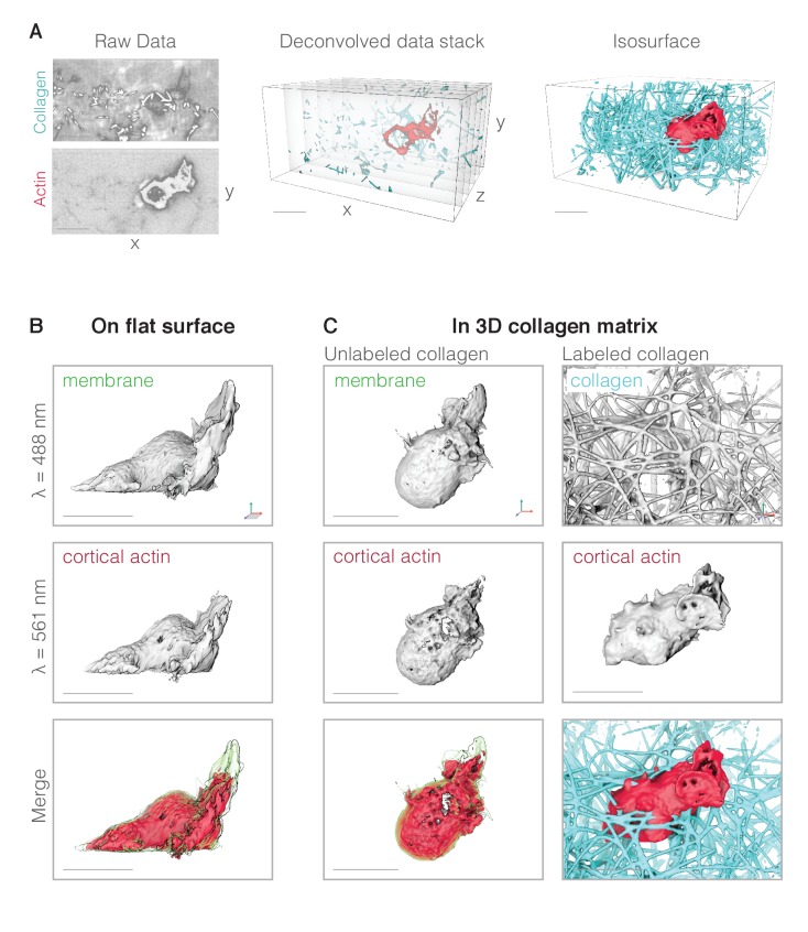
Figure 1.
Data processing and visualization.
( A ) Data processing pipeline. Left: representative example of raw LLSm data showing a single image plane that passes through a neutrophil-like HL-60 cell (bottom panel) migrating through a collagen ...
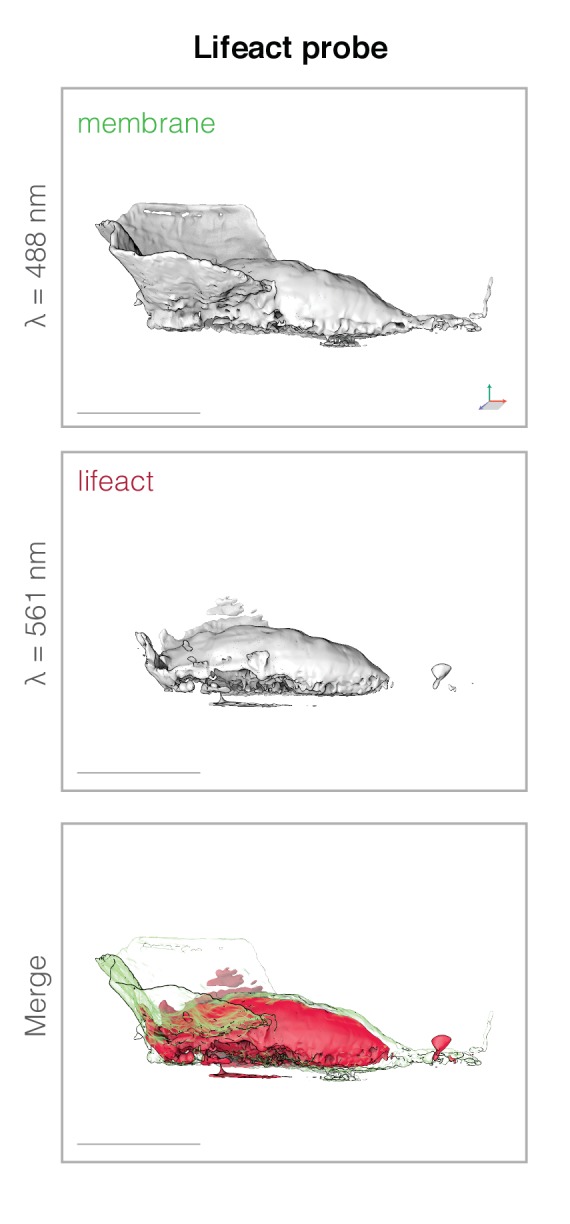
Figure 1u2014figure supplement 1.
A Lifeact-based fluorescent probe does not label filamentous actin in HL-60 pseudopods.
Top: UCSF Chimera rendering of a fluorescence isosurface of a plasma membrane probe (palmitoylated m-Emerald) expressed in a motile HL-60 cell. Middle:a similar surface rendering of mCherry-Lifeact fl...
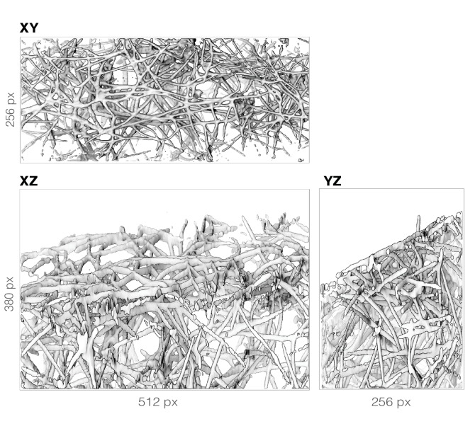
Figure 1u2014figure supplement 2.
Comparison of isosurface views normal to the XY, YZ, and XZ imaging planes, illustrating the near-isotropic resolution of lattice light sheet microscopy.
Top panel: three-dimensional surface rendering of fluorescein-conjugated collagen fluorescence, oriented so that the viewing angle is normal to the microscope image plane (XY), and parallel to the opt...
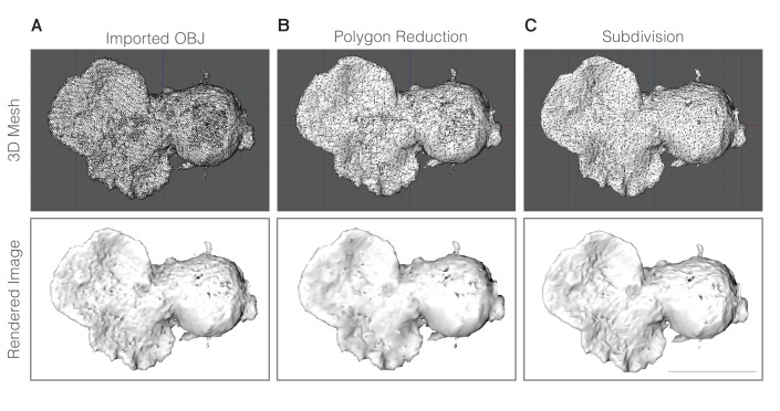
Figure 1u2014figure supplement 3.
Mesh processing for figures, showing both the polygon counts (or u2018three-dimensional Meshu2019) and the rendered images.
( A ) Initial Wavefront file exported from UCSF Chimera. ( B ) Results of applying the polygon reduction tool in Cinema4D. ( C ) Final version using Polygon Subdivison, a method of calculating a smoot...
Video 1.
Example of lamellar pseudopods formed by cells crawling on a flat surface (fibronectin-coated glass coverslip).u00a0Videou00a0plays at 10.5u00a0u00d7u00a0real time.
Video 2.
Anotheru00a0example of lamellar pseudopods formed by cells crawling on a flat surface (fibronectin-coated glass coverslip).
Video plays at 11 u00d7 real time. See also Video 1 .
Video 3.
Example where sheets never come into contact with surface.
Because the sample is held vertically in the imaging chamber, edges of cells falling off of the coverslip can pass through the field of view, seen here as objects flowing from right to left. Videou00a...
Video 4.
Anotheru00a0example where sheets never come into contact with surface.
Video plays at 11 u00d7 real time. See also Video 3 .
Video 5.
Example of lamellar pseudopods formed by cells crawling through three-dimensional collagen networks.u00a0Videou00a0plays at 9.5u00a0u00d7u00a0real time.
Video 6.
Anotheru00a0example of lamellar pseudopods formed by cells crawling through three-dimensional collagen networks.
Please note thatu00a0the stage is repositioned several times because the cell migrates out of the field of view.u00a0Video plays at 10 u00d7 real time. See also Video 5 .
Video 7.
Example of u2018rosetteu2019 pseudopods built by cells crawling on flat surface (fibronectin-coated glass coverslips). Video 7 plays at 11u00a0u00d7u00a0real time.
Video 8.
Anotheru00a0exampleu00a0of u2018rosetteu2019 pseudopods built by cells crawling on flat surface (fibronectin-coated glass coverslips).
Video plays at 11 u00d7 real time. See also Video 7 .
Video 9.
Example of u2018rosetteu2019 pseudopods built by cells crawling through polymerized collagen networks.
Videou00a0plays at 11u00a0u00d7u00a0real time.
Video 10.
Anotheru00a0exampleu00a0of u2018rosetteu2019 pseudopods built by cells crawling through polymerized collagen networks.
Video plays at 10 u00d7 real time. See also Video 9 .
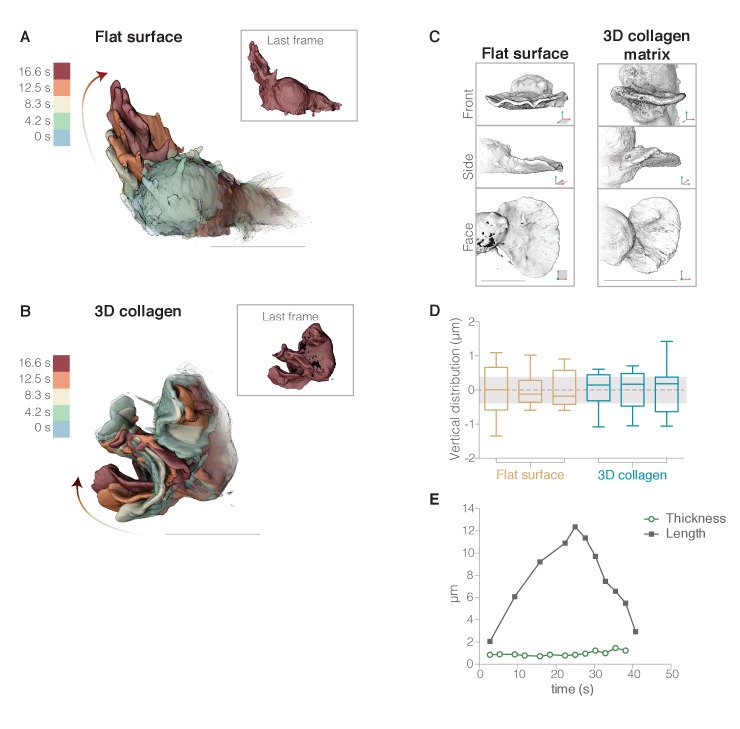
Figure 2.
Neutrophils form lamellar pseudopods regardless of whether they are crawling on two-dimensional surfaces or moving through complex three-dimensional environments.
( Au2013B ) To illustrate the morphology of rapidly growing membrane protrusions we overlaid multiple fluorescence iso-surface images taken at different time points of individual HL-60 cells expressin...
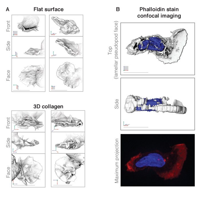
Figure 2u2014figure supplement 1.
Neutrophils form lamellar pseudopods.
( A ) Additional three-dimensional visualizations of single time points from four independent cells (two on glass and two in matrix) forming lamellar pseudopods shown en face, from the side, and from ...
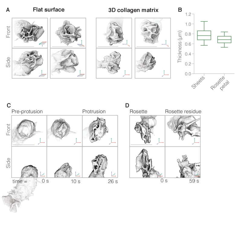
Figure 3.
Neutrophils build complex pseudopods (u2018rosettesu2019) formed of multiple lamellar sheets.
( A ) Three-dimensional visualizations of rosettes built by cells crawling on two-dimensional surfaces (left) as well as through unlabeled collagen meshes (right). Single timepoints of two independent...
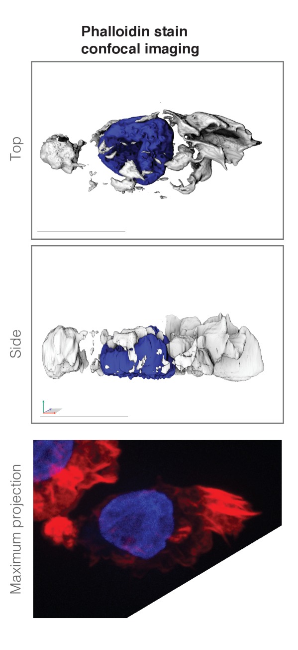
Figure 3u2014figure supplement 1.
Spinning disk confocal image of fixed cell with a complex rosette pseudopod.
The resulting three-dimensional stack was rendered in UCSF Chimera, with a top (X,Y) view and side (Z,Y) view shown. (Bottom) Maximum intensity projection of phalloidin staining (red) reveals rosette ...
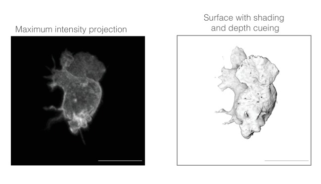
Figure 3u2014figure supplement 2.
Maximum intensity projection of deconvolved lattice light sheet microscopy data (left) compared to surface rendering (right).
This particular time point was chosen to highlight the need for appropriate visualization tools to determine spatial relationships between structures protruding from the cell surface.
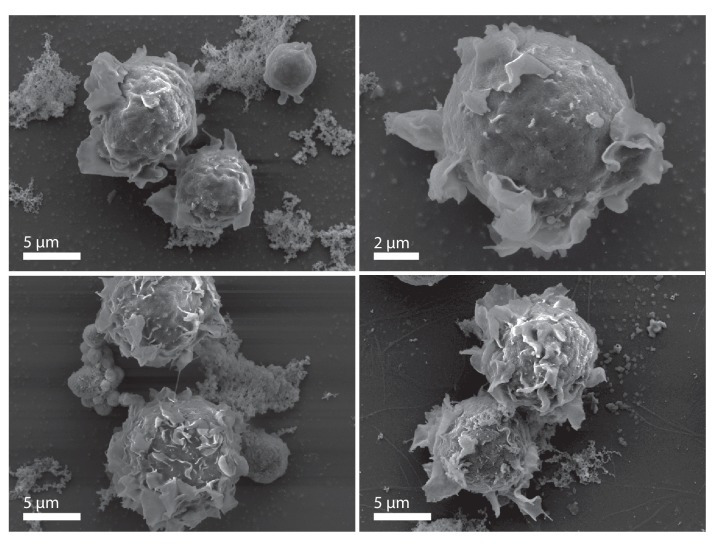
Figure 3u2014figure supplement 3.
Scanning electron micrographs of Jurkat T cells on coverslips.
Planar protrusions on these lymphocytes are reminiscent of those we observe in HL-60 cells. Scale baru00a0=u00a02 u00b5m for top right panel and 5 u00b5m for other panels.
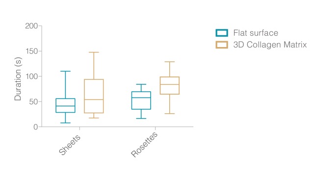
Figure 3u2014figure supplement 4.
Box and whisker plot of lifetimes of simple (left) and rosette (right) pseudopods built by cells crawling across coated glass surfaces (blue) and through collagen meshes (brown).
Nine cells were analyzed from three independent experiments.
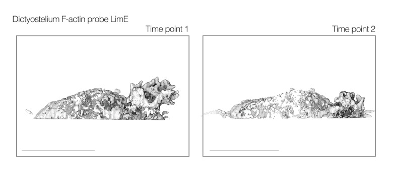
Figure 3u2014figure supplement 5.
UCSF Chimera visualization of two time points of published Dictyostelium cell dataset imaged using Bessel beam microscopy ( Gao et al., 2014 ) showing rosette-like protrusions.
Cell is expressing the Dictyostelium F-actin probe LimE ( Gao et al., 2014 ). Scale baru00a0=u00a010 u00b5m.
Video 11.
Example of CK-666 treated cells migrating through a polymerized collagen network.
Videou00a0plays at 11u00a0u00d7u00a0real time.
Video 12.
Anotheru00a0exampleu00a0of CK-666 treated cells migrating through a polymerized collagen network.
Video plays at 11 u00d7 real time. See also Video 11 .
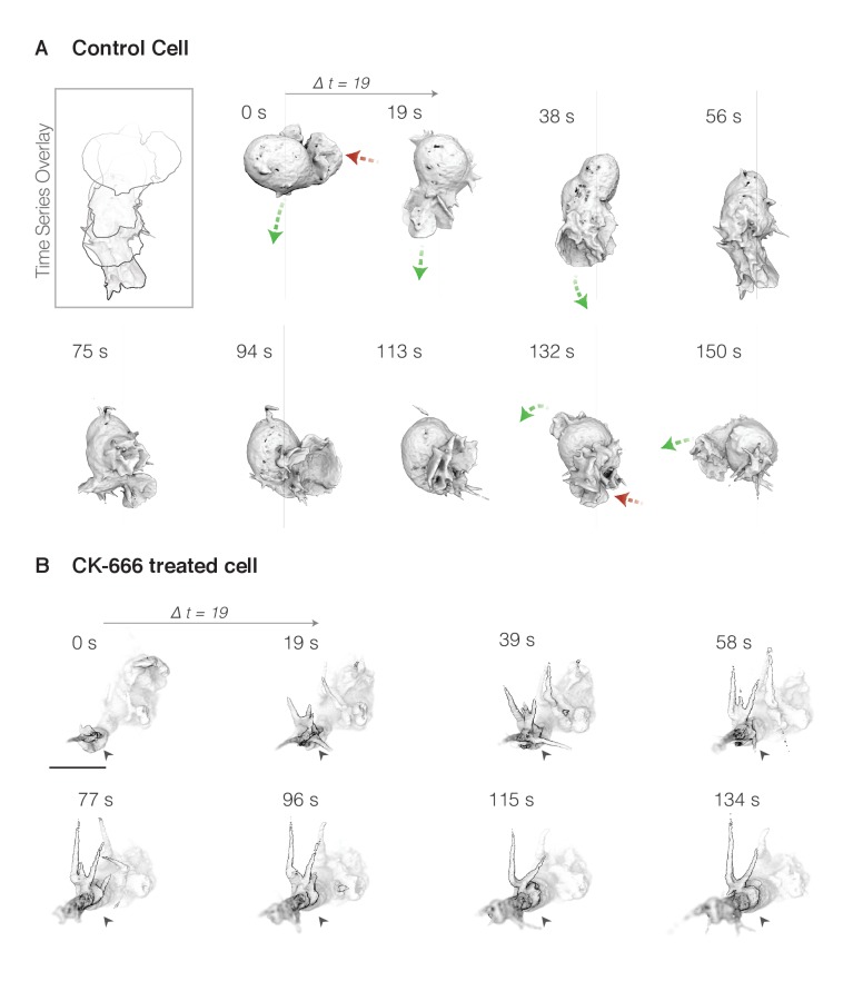
Figure 4.
Both simple lamellar and rosette pseudopods are formed de novo from the cell body and require Arp2/3 activity for assembly.
( A ) Surface rendering of membrane-labeled control HL-60 cell atu00a0~19 s intervals. Green arrows highlight growing pseudopods, while shrinking pseudopods are indicated by red arrows. Inset (top lef...
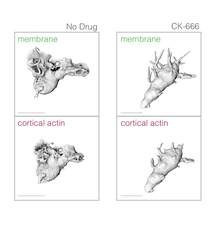
Figure 4u2014figure supplement 1.
Comparison of protrusions formed by control (Left column) and CK-666 treated (Right column) cells expressing both membrane (Top row) and cortical actin Utrophin-based actin probes (Bottom row).
Video 13.
Videos of WAVE fluorescence in TIRF (left) and ventral cell surface distance from the glass coverslip in RICM (middle), and overlay (right).
For RICM, dark areas represent larger distances between the coverslip and the ventral cell surface; bright white (or magenta, in the overlay) indicates close contact of the cell onto the glass. Two di...
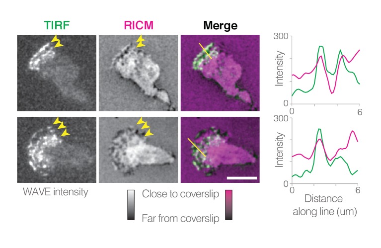
Figure 5.
WAVE complex localizes to ventral protrusions.
Time-lapse images of WAVE complex fluorescence in TIRF (left) and ventral cell surface distance from the glass coverslip in reflective interference contrast microscopy (RICM, middle), and overlay (rig...
Video 14.
Video highlighting automation of protrusion detection in control cells.u00a0Videou00a0plays at 10u00a0u00d7u00a0real time.
Video 15.
Video 15 Video highlighting automation of protrusion detection in CK666 cells.u00a0Videou00a0plays at 11u00a0u00d7u00a0real time.
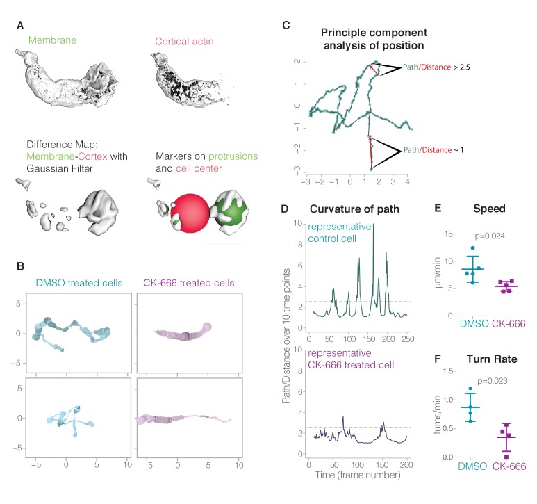
Figure 6.
Lamellar pseudopods are associated with cell turning, but are not required for locomotion.
( A ) Automatic pseudopod detection relies on the relative exclusion of the Utrophin-based actin probe from the dynamic actin networks within pseudopods; pseudopods are identified by first subtracting...
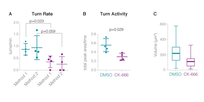
Figure 6u2014figure supplement 1.
Calculating turning points ( A ) Turn rates (calculated by two distinct methods) of control cells (nu00a0=u00a04 cells over a total of 20.7 min, from at least two independent experiments) and CK-666 treated cells (nu00a0=u00a05 cells over a total of 13.7 min, from at least two independent experiments).
Error bars represent standard deviation. ( B ) Comparison of Turn Activity , calculated as the area under the curvature-of-path plots for the cells shown in ( A ). Error bars represent standard deviat...
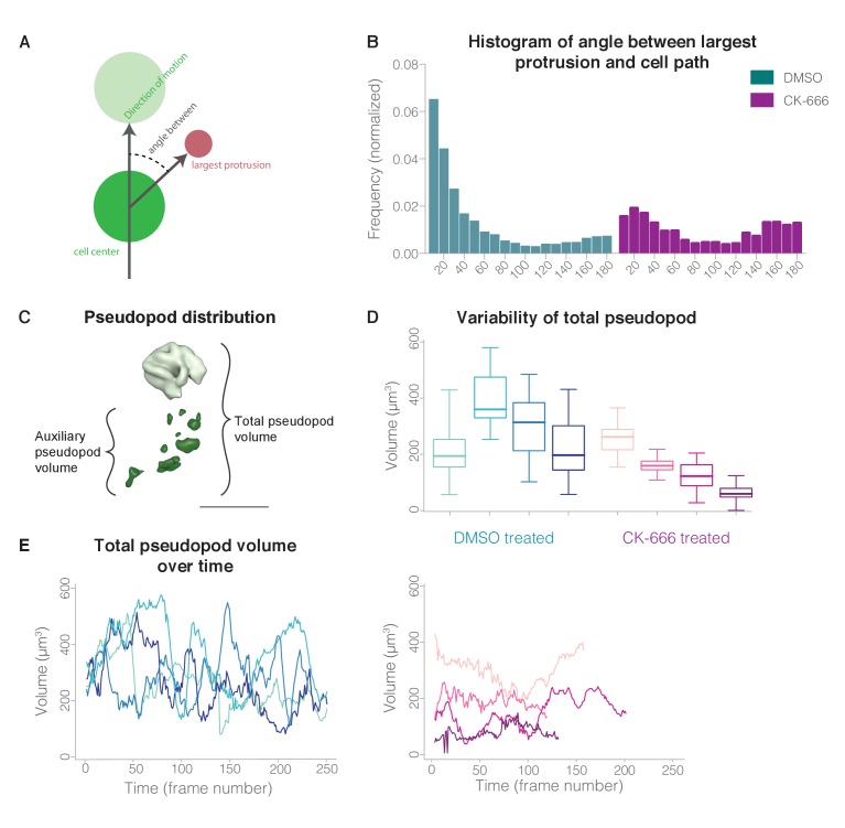
Figure 6u2014figure supplement 2.
Effects of Arp2/3 inhibitor on pseudopod behavior.
( A ) Schematic showing how the angle between main pseudopod and cell path is calculated. ( B ) Comparison of angle between the largest pseudopod and the cell motion trajectory for control and CK-666 ...
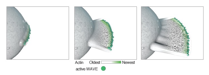
Figure 7.
Model showing how localization of Arp2/3 activator (activated WAVE complex, green) could result in the formation of a lamellar protrusion independent of surface interactions.
Once formed, a flat protrusion would continue growth as a planar projection as described ( Schmeiser and Winkler, 2015 ).
Figure images are served from the NIH/NLM PubMed Central Open Access Subset or Europe PMC; copyright remains with the publishers and authors.
💬 Discussion
0 commentsNo comments yet. Be the first to start a discussion!
Leave a Comment