Abstract
Abstract In the Drosophila antenna, different subtypes of olfactory receptor neurons (ORNs) housed in the same sensory hair (sensillum) can inhibit each other non-synaptically. However, the mechanisms underlying this underexplored form of lateral inhibition remain unclear. Here we use recordings from pairs of sensilla impaled by the same tungsten electrode to demonstrate that direct electrical (“ephaptic”) interactions mediate lateral inhibition between ORNs. Intriguingly, within individual sensilla, we find that ephaptic lateral inhibition is asymmetric such that one ORN exerts greater influence onto its neighbor. Serial block-face scanning electron microscopy of genetically identified ORNs and circuit modeling indicate that asymmetric lateral inhibition reflects a surprisingly simple mechanism: the physically larger ORN in a pair corresponds to the dominant neuron in ephaptic interactions. Thus, morphometric differences between compartmentalized ORNs account for highly specialized inhibitory interactions that govern information processing at the earliest stages of olfactory coding.
🔬 Techniques
🔭 Microscopes
🧬 Organisms
✨ Fluorophores
🧪 Sample Preparation
🏭 Microscope Brands
🧪 Reagent Suppliers
📷 Detectors
💻 Software Details
💾 Data Repositories
🏛️ Research Organizations (ROR)
Affiliated research institutions:
📋 Methods
Drosophila stocks
Flies were raised on standard cornmeal medium at 25 °C, ~60% relative humidity in an incubator with a 12-h light/dark cycle. Female CS flies 5–7 days post eclosion were used in all experiments unless noted otherwise. For the ablation ( UAS-rpr ) and optogenetic ( UAS-H134R-ChR2 ) experiments, 5-day-old females were used; for the SBEM ( UAS-APEX2 ) experiments, 6–8-day-old females were used. For further information on genotypes, refer to Supplementary Table 4 .
Single-sensillum recordings
A fly was wedged into the narrow end of a truncated plastic 200-μl pipette tip to expose the antenna, which was subsequently stabilized between a tapered glass microcapillary tube and a coverslip covered with double-sided type 54 . Single-unit recordings were performed as follows. Briefly, electrical activity of the ORNs was recorded extracellularly by placing a sharp electrode filled with 0.6× sensillum lymph Ringer solution 31 into a sensillum and the reference electrode filled with the same Ringer solution was placed in the eye or the clypeus (for at4 recordings). For recordings performed with a tungsten electrode, a tungsten rod (0.01 × 3 inch, 717000, A-M Systems) secured in an electrode holder (ST50-BNC, Syskiyou) was sharpened in 0.5 N NaOH with a microelectrode etcher (EE-1D, Bak Electronics) at 24 V for nine cycles. No more than three sensilla from the same antenna were recorded. All measurements were taken from distinct neurons except for recordings performed using the bridged configuration shown in Fig. 1b (top and middle panels) and Supplementary Fig. 1 . AC signals (100–20k Hz) and DC signals were simultaneously recorded on an NPI EXT-02F amplifier (ALA Scientific Instruments) and digitized at 5 kHz with Digidata 1550 (Molecular Devices). ORN spikes were detected and sorted using threshold search under Event Detection in Clampfit 10 (Molecular Devices). Spike timing data were exported and analyzed in Igor Pro 6.3 (Wavemetrics). Peri-stimulus time histograms were obtained by averaging spike activities in 50-ms bins and smoothed using a binomial filter (Igor Pro 6.3, Wavemetrics). Sensillum types were identified based on their locations on the antenna or maxillary palp, and their characteristic odor response profiles 15 , 21 . For ac3I and ac3II sensilla, sensillum types were determined according to ORN-specific fluorescent labeling (ac3I: Ir75b-GAL4 ; ac3II: Ir75c-GAL4 ) because the response profiles for ac3I and ac3II in D. melanogaster are virtually indistinguishable 27 . Based on the location of the fluorescence signals, we recorded from ac3I with a medial mounting position and ac3II with a posterior mounting position 55 . Odor stimuli Chemicals were >99% pure or of the highest purity available at Sigma-Aldrich unless otherwise specified. Odorants were diluted in paraffin oil unless otherwise noted. Apple cider vinegar (Spectrum, naturals filtered apple cider vinegar) and geosmin were diluted in water, and trans -palmitoleic acid (Cayman Chemical) was diluted in ethanol. For odor mixture experiments, individual odorants (2× stock solutions) were mixed either with paraffin oil or with another odorant at 1:1 (v/v) ratio prior to experiments. For short odor pulses, odor stimuli (100 μl applied to a filter disc) were delivered from a Pasteur pipette via a pulse of air (200 ml min −1 ) into the main air stream (2000 ml min −1 ). A Pasteur pipette filled with pure (Fig. 1 and Supplementary Fig. 1 ) or diluted CO 2 (5×10 −2 , v/v in air, Supplementary Fig. 6 ) was used to deliver CO 2 stimuli into the main air stream. Background odor stimuli were delivered from a 125-ml flask containing 3 ml of odor dilutions directly downstream of the main air stream (2000 ml min −1 ). For palmitoleic acid, 4.5 μl of the freshly diluted odorant was applied to filter paper inserted inside a truncated 200-µl pipette tip. Ethanol was allowed to evaporate for 1 h in a vacuum desiccator prior to experiments. The odor cartridge was positioned around 4 mm away from the antenna as described 54 . Odor stimulus was delivered via a 500-ms pulse of air (500 ml min −1 ) directly at the antenna in the presence of humidified air flow at 2000 mlmin −1 from a different direction. Of note, female at4A does not respond to palmitoleic acid as strongly as male at4A in 7-day-old flies (Ng et al., unpublished data).
Show full methods section
Drosophila stocks
Flies were raised on standard cornmeal medium at 25 °C, ~60% relative humidity in an incubator with a 12-h light/dark cycle. Female CS flies 5–7 days post eclosion were used in all experiments unless noted otherwise. For the ablation ( UAS-rpr ) and optogenetic ( UAS-H134R-ChR2 ) experiments, 5-day-old females were used; for the SBEM ( UAS-APEX2 ) experiments, 6–8-day-old females were used. For further information on genotypes, refer to Supplementary Table 4 .
Single-sensillum recordings
A fly was wedged into the narrow end of a truncated plastic 200-μl pipette tip to expose the antenna, which was subsequently stabilized between a tapered glass microcapillary tube and a coverslip covered with double-sided type 54 . Single-unit recordings were performed as follows. Briefly, electrical activity of the ORNs was recorded extracellularly by placing a sharp electrode filled with 0.6× sensillum lymph Ringer solution 31 into a sensillum and the reference electrode filled with the same Ringer solution was placed in the eye or the clypeus (for at4 recordings). For recordings performed with a tungsten electrode, a tungsten rod (0.01 × 3 inch, 717000, A-M Systems) secured in an electrode holder (ST50-BNC, Syskiyou) was sharpened in 0.5 N NaOH with a microelectrode etcher (EE-1D, Bak Electronics) at 24 V for nine cycles. No more than three sensilla from the same antenna were recorded. All measurements were taken from distinct neurons except for recordings performed using the bridged configuration shown in Fig. 1b (top and middle panels) and Supplementary Fig. 1 . AC signals (100–20k Hz) and DC signals were simultaneously recorded on an NPI EXT-02F amplifier (ALA Scientific Instruments) and digitized at 5 kHz with Digidata 1550 (Molecular Devices). ORN spikes were detected and sorted using threshold search under Event Detection in Clampfit 10 (Molecular Devices). Spike timing data were exported and analyzed in Igor Pro 6.3 (Wavemetrics). Peri-stimulus time histograms were obtained by averaging spike activities in 50-ms bins and smoothed using a binomial filter (Igor Pro 6.3, Wavemetrics). Sensillum types were identified based on their locations on the antenna or maxillary palp, and their characteristic odor response profiles 15 , 21 . For ac3I and ac3II sensilla, sensillum types were determined according to ORN-specific fluorescent labeling (ac3I: Ir75b-GAL4 ; ac3II: Ir75c-GAL4 ) because the response profiles for ac3I and ac3II in D. melanogaster are virtually indistinguishable 27 . Based on the location of the fluorescence signals, we recorded from ac3I with a medial mounting position and ac3II with a posterior mounting position 55 . Odor stimuli Chemicals were >99% pure or of the highest purity available at Sigma-Aldrich unless otherwise specified. Odorants were diluted in paraffin oil unless otherwise noted. Apple cider vinegar (Spectrum, naturals filtered apple cider vinegar) and geosmin were diluted in water, and trans -palmitoleic acid (Cayman Chemical) was diluted in ethanol. For odor mixture experiments, individual odorants (2× stock solutions) were mixed either with paraffin oil or with another odorant at 1:1 (v/v) ratio prior to experiments. For short odor pulses, odor stimuli (100 μl applied to a filter disc) were delivered from a Pasteur pipette via a pulse of air (200 ml min −1 ) into the main air stream (2000 ml min −1 ). A Pasteur pipette filled with pure (Fig. 1 and Supplementary Fig. 1 ) or diluted CO 2 (5×10 −2 , v/v in air, Supplementary Fig. 6 ) was used to deliver CO 2 stimuli into the main air stream. Background odor stimuli were delivered from a 125-ml flask containing 3 ml of odor dilutions directly downstream of the main air stream (2000 ml min −1 ). For palmitoleic acid, 4.5 μl of the freshly diluted odorant was applied to filter paper inserted inside a truncated 200-µl pipette tip. Ethanol was allowed to evaporate for 1 h in a vacuum desiccator prior to experiments. The odor cartridge was positioned around 4 mm away from the antenna as described 54 . Odor stimulus was delivered via a 500-ms pulse of air (500 ml min −1 ) directly at the antenna in the presence of humidified air flow at 2000 mlmin −1 from a different direction. Of note, female at4A does not respond to palmitoleic acid as strongly as male at4A in 7-day-old flies (Ng et al., unpublished data).
Optogenetic stimulation
Newly eclosed female flies expressing the H134R-ChR2 transgene in target ORNs were reared in constant darkness for 5 days on fly food supplemented with 100 μM all trans -retinal (Sigma) unless otherwise specified. Flies were transferred to fresh retinal food 1 day prior to experiments. A light stimulus was generated via a blue LED (470 nm, Universal LED Illumination System, pE-4000, Cool LED). Light pulses (500-ms duration) were controlled by a shutter (Vincent Associates) driven by Clampex 10.4 (Molecular Devices). Light output around the position of the recorded antenna was measured with an optical power meter (PMKIT-05-01, Newport Corporation) via a slim profile wand detector (818-ST2/DB, Newport Corporation). The LFP light responses in the ac3 neurons expressing H134R-ChR2 were too small to be reliably analyzed. Attempts to express H134R-ChR2 in ab5A (Or82a-GAL4) or ab5B (Or47a-GAL4) failed to yield any light responses, despite the observation that the fluorescence of mCherry tag on H134-ChR2 was visible in the target ORNs. Aging the transgenic flies to 14 days old or increasing retinal concentrations in the food did not improve the situation.
Immunohistochemistry Seven-day-old female files expressing myc-tagged
Orco and/or Or85a odorant receptors in the ab2B ORNs were anesthetized on ice, with their heads aligned in a collar, covered with Cryo-OCT (Tissue-Tek, Fisher Scientific), and frozen on dry ice 56 . Cryosections (14μm) were fixed with 4% paraformaldehyde in 1× phosphate-buffered saline and stained with rabbit anti-myc antibody (1:250, 71D10, Cell Signaling Technology) and 21A6 (ciliary base marker, 1:200, DSHB), followed by goat anti-rabbit Alexa 647 secondary antibody (1:250, A21236, Life Technologies) and goat anti-mouse Alexa 568 (1:200, A11019, Life Technologies). Confocal microscopy was performed with a Zeiss 880 Airyscan Microscope, and images were processed with ImageJ software.
Sample preparation for SBEM
Target expression of APEX2 in ORNs for SBEM was performed as follows 46 . Briefly, transgenic Drosophila lines ( 10xUAS-myc-APEX2-Orco or 10xUAS-mCD8GF-APEX2 ) were generated to facilitate dendritic targeting of APEX2 46 .
Expression of APEX2 in select
ORNs was driven by OrX-GAL4 drivers (Supplementary Data 1 ). Six- to eight-day-old female flies were cold anesthetized prior to the dissection of their antennae. The antennae were processed with the CryoChem method 46 , which involves cryofixation by high-pressure freezing, freeze-substitution, rehydration, DAB labeling reaction, en bloc heavy metal staining, dehydration, and resin infiltration. Microcomputed X-ray tomography was performed on resin-embedded specimens using a Versa 510 X-ray microscope (Zeiss) to determine DAB-labeled region of interest. The specimens were then mounted on aluminum pins with conductive silver epoxy (Ted Pella) and sputter coated with gold-palladium for SBEM imaging. The ab3, ab4, ac3II, at4 datasets were collected with a Gemini SEM (Zeiss) equipped with a 3View block-face unit (Gatan); the ab5 dataset was collected with a Merlin scanning electron microscope (Zeiss) equipped with a 3View2XP and OnPoint backscatter detector (Gatan). Parameters for SBEM image acquisition are listed in Supplementary Table 5 .
Segmentation of DAB-labeled Drosophila ORNs The DAB-labeled Drosophila
ORN was segmented in a semi-automated fashion using the IMOD software 57 to generate a 3D model 46 . The IMOD command line “imodauto” was used for the auto-segmentation by setting thresholds to isolate the labeled neuron of interest. Auto-segmentation was followed by manual proofreading and correction of errors by two independent proofreaders. The neighboring, unlabeled ORN was manually segmented using the same software. Due to insufficient DAB labeling, the fine outer dendritic branches of most basiconic ORNs could not be reliably identified for segmentation. Morphometric analysis The 3D model of each ORN was first separated into cell body, inner dendrite and outer (sensory) dendrite models. The inner and outer dendrites were separated at the cilium base, a notably constricted dendritic region 42 . The volume measurements of ORNs were then obtained with the “imodinfo” function in IMOD based on the 3D models. The lengths of most inner and outer dendrites were determined by first converting the 3D models into binary image files using the IMOD command “imodmop”. Then the skeletons of the 3D images were extracted using Skeletonize3D ( https://imagej.net/Skeletonize3D ) plugin in Fiji (NIH). The lengths of the resulting skeletons were obtained by the Fiji “Analyze Skeleton” function. For the ab3A, ab4A and ab5A ORNs, which exhibit significant dendritic enlargements (Fig. 6f ), their inner dendritic lengths were determined by first visually identifying the center point in every ninth contour of the 3D models (300~400 nm z-step), then manually measuring and summing the distances between those points. The inner dendritic lengths of the ab3B, ab4B, and ab5B ORNs were determined in the same way. The outer dendritic lengths reported in Supplementary Table 2 are the distances between the cilium bases and the tips of the longest dendritic branch. The outer dendrites of ORNs were assumed to be cylindrical and their surface areas were calculated based on the measured volumes and lengths accordingly. The surface areas of cell bodies were measured with the “imodinfo” function in IMOD.
Statistics
All data presented as mean ± s.e.m. were analyzed using Igor Pro 6.3 or SigmaPlot 13.0. Coefficients and the standard deviations of the linear fits were generated in Igor Pro 6.3. Unpaired two-tailed t test was performed in Supplementary Fig. 8 for single variable comparison between two groups. Paired two-tailed t test was performed in Fig. 6 for the morphological comparison between grouped ORNs. Data are presented as mean ± s.e.m. P < 0.05 was considered to be statistically significant and is presented as ∗ P < 0.05, ∗∗ P < 0.01, or ∗∗∗ P < 0.001. Statistical significance for linear coefficients was determined by analysis of covariance (ANCOVA) in RStudio using functions within the car package (version3.0-0). Data are presented as coefficient ± s.d. P < 0.05 was considered to be statistically significant and the differences are denoted by different letters.
Modeling
We consider the passive electric circuit model containing an auxiliary cell (denoted “A”) and two ORNs (ORN 1 and ORN 2 ) (Fig. 7a ). Each cell is modeled as an effective Thevenin circuit with battery and resistances. The auxiliary cell is modeled as a battery E A in line with an input resistance R A . The soma of ORN 1 is modeled as a battery E 1 with input resistance R in1 , and the sensory dendrite is modeled as an odorant stimulation-dependent resistance R d1 (similar for ORN 2 ). The driving forces for the currents are the batteries E A , E 1 and E 2 . The voltage V A is the transepithelium potential, and V m1 and V m2 are the neuronal transmembrane potentials that control spike firing. Changes in V A are recorded as changes in the local field potential, LFP. Of note, this passive electric circuit model concerns voltage changes resulting from constant odor stimulation. Therefore, all capacitive currents are considered zero in this model. The system of equations for the currents I A , I 1 and I 2 reads 1 documentclass[12pt]{minimal} usepackage{amsmath} usepackage{wasysym} usepackage{amsfonts} usepackage{amssymb} usepackage{amsbsy} usepackage{mathrsfs} usepackage{upgreek} setlength{oddsidemargin}{-69pt} begin{document}$${V_{mathrm{{A}}}} = {E_{mathrm{{A}}} + I_{mathrm{{A}}}R_{mathrm{{A}}}},\ {V_{mathrm{{A}}}} = {E_1 + I_1R_1},\ {V_{mathrm{{A}}}} = {E_2 + I_2R_2},\ 0 = {I_{mathrm{{A}}} + I_1 + I_2},$$end{document} V A = E A + I A R A , V A = E 1 + I 1 R 1 , V A = E 2 + I 2 R 2 , 0 = I A + I 1 + I 2 , where we introduce the total resistances R 1 = R in1 + R d1 and R 2 = R in2 + R d2 . By solving these equations, we obtain the currents 2 documentclass[12pt]{minimal} usepackage{amsmath} usepackage{wasysym} usepackage{amsfonts} usepackage{amssymb} usepackage{amsbsy} usepackage{mathrsfs} usepackage{upgreek} setlength{oddsidemargin}{-69pt} begin{document}$$begin{array}{*{20}{c}} {I_{mathrm{{A}}}} & = & {frac{{E_1frac{{R_2}}{{R_1 + R_2}} + E_2frac{{R_1}}{{R_1 + R_2}} - E_{mathrm{{A}}}}}{{frac{{R_1R_2}}{{R_1 + R_2}} + R_{mathrm{{A}}}}}}, \ {I_1} & = & {frac{{E_2 - E_1}}{{R_1 + R_2}} - I_{mathrm{{A}}}frac{{R_2}}{{R_1 + R_2}}}, \ {I_2} & = & {frac{{E_1 - E_2}}{{R_1 + R_2}} - I_{mathrm{A}}frac{{R_1}}{{R_1 + R_2}}}. end{array}$$end{document} I A = E 1 R 2 R 1 + R 2 + E 2 R 1 R 1 + R 2 - E A R 1 R 2 R 1 + R 2 + R A , I 1 = E 2 - E 1 R 1 + R 2 - I A R 2 R 1 + R 2 , I 2 = E 1 - E 2 R 1 + R 2 - I A R 1 R 1 + R 2 . The neuronal part is an effective Thevenin circuit with battery documentclass[12pt]{minimal} usepackage{amsmath} usepackage{wasysym} usepackage{amsfonts} usepackage{amssymb} usepackage{amsbsy} usepackage{mathrsfs} usepackage{upgreek} setlength{oddsidemargin}{-69pt} begin{document}$$E_{mathrm{T}} = E_1frac{{R_2}}{{R_1 + R_2}} + E_2frac{{R_1}}{{R_1 + R_2}}$$end{document} E T = E 1 R 2 R 1 + R 2 + E 2 R 1 R 1 + R 2 and resistance documentclass[12pt]{minimal} usepackage{amsmath} usepackage{wasysym} usepackage{amsfonts} usepackage{amssymb} usepackage{amsbsy} usepackage{mathrsfs} usepackage{upgreek} setlength{oddsidemargin}{-69pt} begin{document}$$R_{mathrm{T}} = frac{{R_1R_2}}{{R_1 + R_2}}$$end{document} R T = R 1 R 2 R 1 + R 2 . The neuronal membrane potentials are 3 documentclass[12pt]{minimal} usepackage{amsmath} usepackage{wasysym} usepackage{amsfonts} usepackage{amssymb} usepackage{amsbsy} usepackage{mathrsfs} usepackage{upgreek} setlength{oddsidemargin}{-69pt} begin{document}$$begin{array}{*{20}{r}} hfill {V_{{mathrm{m}}1}} & hfill = & hfill {E_1 + R_{{mathrm{{in}}}1}I_1},\ hfill {} & hfill {} & hfill {}\ hfill {V_{{mathrm{m}}2}} & hfill = & hfill {E_2 + R_{{mathrm{{in}}}2}I_2}.end{array}$$end{document} V m 1 = E 1 + R in 1 I 1 , V m 2 = E 2 + R in 2 I 2 . To further simplify the analysis, we use R A to define dimensionless resistances documentclass[12pt]{minimal} usepackage{amsmath} usepackage{wasysym} usepackage{amsfonts} usepackage{amssymb} usepackage{amsbsy} usepackage{mathrsfs} usepackage{upgreek} setlength{oddsidemargin}{-69pt} begin{document}$$tilde R_{mathrm{{A}}} = R_{mathrm{{A}}}{mathrm{/}}R_{mathrm{{A}}} = 1$$end{document} R ~ A = R A ∕ R A = 1 , documentclass[12pt]{minimal} usepackage{amsmath} usepackage{wasysym} usepackage{amsfonts} usepackage{amssymb} usepackage{amsbsy} usepackage{mathrsfs} usepackage{upgreek} setlength{oddsidemargin}{-69pt} begin{document}$$tilde R_1 = R_1{mathrm{/}}R_{mathrm{{A}}}$$end{document} R ~ 1 = R 1 ∕ R A , documentclass[12pt]{minimal} usepackage{amsmath} usepackage{wasysym} usepackage{amsfonts} usepackage{amssymb} usepackage{amsbsy} usepackage{mathrsfs} usepackage{upgreek} setlength{oddsidemargin}{-69pt} begin{document}$$tilde R_2 = R_2{mathrm{/}}R_{mathrm{{A}}}$$end{document} R ~ 2 = R 2 ∕ R A and rescale currents documentclass[12pt]{minimal} usepackage{amsmath} usepackage{wasysym} usepackage{amsfonts} usepackage{amssymb} usepackage{amsbsy} usepackage{mathrsfs} usepackage{upgreek} setlength{oddsidemargin}{-69pt} begin{document}$$widetilde I_{mathrm{{A}}} = I_{mathrm{{A}}}R_{mathrm{{A}}}$$end{document} I ~ A = I A R A , documentclass[12pt]{minimal} usepackage{amsmath} usepackage{wasysym} usepackage{amsfonts} usepackage{amssymb} usepackage{amsbsy} usepackage{mathrsfs} usepackage{upgreek} setlength{oddsidemargin}{-69pt} begin{document}$$widetilde I_1 = I_1R_{mathrm{{A}}}$$end{document} I ~ 1 = I 1 R A and documentclass[12pt]{minimal} usepackage{amsmath} usepackage{wasysym} usepackage{amsfonts} usepackage{amssymb} usepackage{amsbsy} usepackage{mathrsfs} usepackage{upgreek} setlength{oddsidemargin}{-69pt} begin{document}$$tilde I_{2} = I_{2}R_{mathrm{A}}$$end{document} Ĩ 2 = I 2 R A . This does not affect the voltages in Eqs. 1 and 3 and is formally equivalent to setting R A = 1. In the following, we therefore omit the tilde symbols and simply use R A = 1. As mentioned before, this does not affect the results and conclusions concerning voltages. We next focus on the input and dendritic resistances. We are interested in how odorant stimulation and the morphometric properties of soma and sensory dendrites affect the transmembrane potentials V m1 and V m2 . We assume that the input resistances R in1 and R in2 depend on the size of the soma and a smaller ORN has a higher input resistance compared to a larger ORN. Specifically, we assume that R in1 and R in2 are inversely proportional to the soma surfaces A s1 and A s2 4 documentclass[12pt]{minimal} usepackage{amsmath} usepackage{wasysym} usepackage{amsfonts} usepackage{amssymb} usepackage{amsbsy} usepackage{mathrsfs} usepackage{upgreek} setlength{oddsidemargin}{-69pt} begin{document}$$R_{{mathrm{{in}}}1} = frac{{rho _{mathrm{{s}}}}}{{A_{{mathrm{{s}}}1}}}quad {mathrm{and}}quad R_{{mathrm{{in}}}2} = frac{{rho _{mathrm{{s}}}}}{{A_{{mathrm{{s}}}2}}},$$end{document} R in 1 = ρ s A s 1 and R in 2 = ρ s A s 2 , where ρ s is the soma membrane resistivity. We model the sensory dendrite of an ORN as a uniform cylinder of length L with axial (cytoplasmic) resistivity r a and membrane resistivity r m , where r m depends on odor activation. From linear cable theory, the input resistance R s of a uniform leaky cylinder with an open and a sealed end is 5 documentclass[12pt]{minimal} usepackage{amsmath} usepackage{wasysym} usepackage{amsfonts} usepackage{amssymb} usepackage{amsbsy} usepackage{mathrsfs} usepackage{upgreek} setlength{oddsidemargin}{-69pt} begin{document}$$R_{mathrm{{d}}} = sqrt {r_{mathrm{{m}}}r_{mathrm{{a}}}} {mathrm{coth}}left( {Lsqrt {frac{{r_{mathrm{{a}}}}}{{r_{mathrm{{m}}}}}} }, right)$$end{document} R d = r m r a coth L r a r m , where documentclass[12pt]{minimal} usepackage{amsmath} usepackage{wasysym} usepackage{amsfonts} usepackage{amssymb} usepackage{amsbsy} usepackage{mathrsfs} usepackage{upgreek} setlength{oddsidemargin}{-69pt} begin{document}$$l = Lsqrt {frac{{r_{mathrm{{a}}}}}{{r_{mathrm{{m}}}}}}$$end{document} l = L r a r m is the electrotonic length of the cylinder and documentclass[12pt]{minimal} usepackage{amsmath} usepackage{wasysym} usepackage{amsfonts} usepackage{amssymb} usepackage{amsbsy} usepackage{mathrsfs} usepackage{upgreek} setlength{oddsidemargin}{-69pt} begin{document}$$R_infty = sqrt {r_{mathrm{{m}}}r_{mathrm{{a}}}}$$end{document} R ∞ = r m r a is the input resistance of an infinitely long cylinder. We further simplify Eq. 5 assuming that the cytoplasmic resistance is much smaller than the membrane resistance such that l ≪ 1 58 . By expanding Eq. 5 for l ≪ 1 we get in first order 6 documentclass[12pt]{minimal} usepackage{amsmath} usepackage{wasysym} usepackage{amsfonts} usepackage{amssymb} usepackage{amsbsy} usepackage{mathrsfs} usepackage{upgreek} setlength{oddsidemargin}{-69pt} begin{document}$$R_{mathrm{{d}}} = frac{{r_{mathrm{{m}}}}}{L} = frac{{rho _{mathrm{{d}}}}}{{A_{mathrm{{d}}}}},$$end{document} R d = r m L = ρ d A d , where ρ d is the dendritic membrane resistivity and A d is the dendritic surface. The membrane resistivity ρ d implicitly depends on odor activation because odorants activate receptors that increase the membrane conductivity. We simplify the transduction process and assume that for a given stimulation with odorant concentration “od”, the amount of activated receptors is given by the Hill function 7 documentclass[12pt]{minimal} usepackage{amsmath} usepackage{wasysym} usepackage{amsfonts} usepackage{amssymb} usepackage{amsbsy} usepackage{mathrsfs} usepackage{upgreek} setlength{oddsidemargin}{-69pt} begin{document}$$R^ ast = R_{max}^ ast frac{{{mathrm{{od}}}^n}}{{{mathrm{{od}}}^n + K_{{mathrm{{od}}}}^n}},$$end{document} R * = R max * od n od n + K od n , where n is the Hill-coefficient and K od the odorant concentration that activates half of the receptors. Receptor activation induces the additional membrane conductivity documentclass[12pt]{minimal} usepackage{amsmath} usepackage{wasysym} usepackage{amsfonts} usepackage{amssymb} usepackage{amsbsy} usepackage{mathrsfs} usepackage{upgreek} setlength{oddsidemargin}{-69pt} begin{document}$$sigma _{mathrm{{d}}} = gamma R^ ast = sigma _{{mathrm{{d}}},max}frac{{{mathrm{{od}}}^n}}{{{mathrm{{od}}}^n + K_{{mathrm{{od}}}}^n}}$$end{document} σ d = γ R * = σ d , max od n od n + K od n . With the basal resistivity ρ d,0 , the overall conductivity is documentclass[12pt]{minimal} usepackage{amsmath} usepackage{wasysym} usepackage{amsfonts} usepackage{amssymb} usepackage{amsbsy} usepackage{mathrsfs} usepackage{upgreek} setlength{oddsidemargin}{-69pt} begin{document}$$frac{1}{{rho _{mathrm{{d}}}}} = frac{1}{{rho _{{mathrm{{d}}},0}}} + sigma _{mathrm{{d}}} = frac{{1 + rho _{{mathrm{{d}}},0}sigma _{mathrm{{d}}}}}{{rho _{{mathrm{{d}}},0}}}$$end{document} 1 ρ d = 1 ρ d , 0 + σ d = 1 + ρ d , 0 σ d ρ d , 0 . This gives 8 documentclass[12pt]{minimal} usepackage{amsmath} usepackage{wasysym} usepackage{amsfonts} usepackage{amssymb} usepackage{amsbsy} usepackage{mathrsfs} usepackage{upgreek} setlength{oddsidemargin}{-69pt} begin{document}$$rho _{mathrm{{d}}} = frac{{rho _{{mathrm{{d}}},0}}}{{1 + g}}$$end{document} ρ d = ρ d , 0 1 + g with 9 documentclass[12pt]{minimal} usepackage{amsmath} usepackage{wasysym} usepackage{amsfonts} usepackage{amssymb} usepackage{amsbsy} usepackage{mathrsfs} usepackage{upgreek} setlength{oddsidemargin}{-69pt} begin{document}$$g = g_{max}frac{{{mathrm{{od}}}^n}}{{{mathrm{{od}}}^n + K_{{mathrm{{od}}}}^n}}$$end{document} g = g max od n od n + K od n and documentclass[12pt]{minimal} usepackage{amsmath} usepackage{wasysym} usepackage{amsfonts} usepackage{amssymb} usepackage{amsbsy} usepackage{mathrsfs} usepackage{upgreek} setlength{oddsidemargin}{-69pt} begin{document}$$g_{max} = rho _{{mathrm{{d}}},0}sigma _{{mathrm{{d}}},max}.$$end{document} g max = ρ d , 0 σ d , max . In summary, to model the dendritic resistances we use the formula 10 documentclass[12pt]{minimal} usepackage{amsmath} usepackage{wasysym} usepackage{amsfonts} usepackage{amssymb} usepackage{amsbsy} usepackage{mathrsfs} usepackage{upgreek} setlength{oddsidemargin}{-69pt} begin{document}$$R_{mathrm{{d}}} = frac{{rho _{{mathrm{{d}}},0}}}{{A_{mathrm{{d}}}(1 + g)}}.$$end{document} R d = ρ d , 0 A d ( 1 + g ) . We next address the changes in local field potential due to stimulation of ORN 1 or ORN 2 . When the activation of ORN 1 is altered due to odorant stimulation, the dendritic resistance R d1 changes by Δ R d1 which alters the local field potential LFP by |Δ V A |. From Eqs. 1 to 3 we compute that the corresponding changes in the membrane potentials are documentclass[12pt]{minimal} usepackage{amsmath} usepackage{wasysym} usepackage{amsfonts} usepackage{amssymb} usepackage{amsbsy} usepackage{mathrsfs} usepackage{upgreek} setlength{oddsidemargin}{-69pt} begin{document}$${mathrm{Delta }}V_{{mathrm{{m}}}2} = {mathrm{Delta }}V_{mathrm{{A}}}frac{{R_{{mathrm{{in}}}2}}}{{R_2}}$$end{document} Δ V m 2 = Δ V A R in 2 R 2 and 11 documentclass[12pt]{minimal} usepackage{amsmath} usepackage{wasysym} usepackage{amsfonts} usepackage{amssymb} usepackage{amsbsy} usepackage{mathrsfs} usepackage{upgreek} setlength{oddsidemargin}{-69pt} begin{document}$${mathrm{Delta }}V_{{mathrm{{m}}}1} = - {mathrm{Delta }}V_{mathrm{{A}}}R_{{mathrm{{in}}}1}left( {1 + frac{1}{{R_2}}} right).$$end{document} Δ V m 1 = - Δ V A R in 1 1 + 1 R 2 . Similarly, when ORN 2 is stimulated we have documentclass[12pt]{minimal} usepackage{amsmath} usepackage{wasysym} usepackage{amsfonts} usepackage{amssymb} usepackage{amsbsy} usepackage{mathrsfs} usepackage{upgreek} setlength{oddsidemargin}{-69pt} begin{document}$${mathrm{Delta }}V_{{mathrm{{m}}}1} = {mathrm{Delta }}V_{mathrm{{A}}}frac{{R_{{mathrm{{in}}}1}}}{{R_1}}$$end{document} Δ V m 1 = Δ V A R in 1 R 1 and 12 documentclass[12pt]{minimal} usepackage{amsmath} usepackage{wasysym} usepackage{amsfonts} usepackage{amssymb} usepackage{amsbsy} usepackage{mathrsfs} usepackage{upgreek} setlength{oddsidemargin}{-69pt} begin{document}$${mathrm{Delta }}V_{{mathrm{{m}}}2} = - {mathrm{Delta }}V_{mathrm{{A}}}R_{{mathrm{{in}}}2}left( {1 + frac{1}{{R_1}}} right).$$end{document} Δ V m 2 = - Δ V A R in 2 1 + 1 R 1 . Because R 2 ( R 1 ) remains constant when ORN 1 (ORN 2 ) is stimulated 12 , it follows that Δ V m1 and Δ V m2 change linearly with Δ V A . Assume that ORN 1 corresponds to the larger neuron A and ORN 2 to the smaller neuron B such that R in1 < R in2 and R 1 < R 2 . With this we have documentclass[12pt]{minimal} usepackage{amsmath} usepackage{wasysym} usepackage{amsfonts} usepackage{amssymb} usepackage{amsbsy} usepackage{mathrsfs} usepackage{upgreek} setlength{oddsidemargin}{-69pt} begin{document}$$R_{{mathrm{{in}}}1}( {1 + frac{1}{{R_2}}} ) < R_{{mathrm{{in}}}2}( {1 + frac{1}{{R_1}}} )$$end{document} R in 1 ( 1 + 1 R 2 ) < R in 2 ( 1 + 1 R 1 ) which is in agreement with Fig. 3 showing that the slope of the spiking rate (which reflects Δ V m1 or Δ V m2 ) vs. LFP is smaller for ORN A compared to ORN B . The following sections concern the fitting procedure. We are interested in whether the differences between our electrophysiological measurements can be explained by the morphometric differences among the grouped ORNs. To address this question, we focus on ab3, ab4 and ab5 sensilla for which we have electrophysiological and morphometric data. We simultaneously fitted the combined LFP data (Fig. 2 ) using a minimal model with a common set of basic parameters and ORN-specific parameters (surface area and odorant sensitivity). In the following, we derive the minimal model that we use for the fitting procedure. For values of fitting parameters, see Tables 1 – 3 . The fitting and simulation results are presented in Fig. 7 of the main text. Table 1 ORN-specific morphometric parameters ORN type Surface area (μm 2 ) Soma Sensory dendrite ab3 A 98 46 B 91 16 ab4 A 137 38 B 75 25 ab5 A 65 20 B 67 20 Measured input parameters are in non-bold (see also Supplementary Table 2), and fitted values in bold Table 2 ORN-specific odorant sensitivities ORN type k od ab3 A −4.8 B −5.1 ab4 A −5.9 B −2.5 ab5 A −1 B −2 Table 3 Common parameters Parameters Description Values E A (mV) Auxiliary cell battery 77 V 0 (mV) ORN resting membrane potential −60 ρ s (μm 2 ) ORN soma membrane resistivity, rescaled by R A 30 ρ d , 0 (μm 2 ) ORN sensory dendrite basal membrane resistivity, rescaled by R A 17 n ORN Hill-coefficient for odorant activation 0.7 g max = ρ d,0 σ d , max . Where σ d,max is the maximum dendritic membrane conductivity induced by receptor activation 10 We were able to fit the combined LFP measurements of ab3, ab4, and ab5 neurons by assuming a common set of parameters that differs only in the areas of soma and sensory dendrite. However, we could not adequately fit the combined LFP data of ac3II, ab3, ab4 and ab5 neurons by assuming such common set of parameters. We note that basiconic ORNs (ab3, ab4, ab5) have highly branched sensory dendrites, whereas coeloconic ORNs do not (ac3II). It is possible that the branching pattern of sensory dendrites or other unknown factors may have introduced additional parameters that affect the fitting results. To estimate the batteries E 1 and E 2 using the resting membrane potential, we assume that the auxiliary cell is the same for all sensillum types, and therefore use a single value for E A . For E 1 and E 2 , we do not assume that they are identical for all sensilla because ORN basal resistances differ depending on the morphometric feature of the neuron, and using the same E 1 and E 2 for all sensilla would lead to different resting membrane potentials for the ORNs (data not shown). This is problematic if one assumes that the mechanism of action potential generation is similar in all ORNs. Instead, we assume that at rest without odorant stimulation (basal condition) the membrane potentials of the ORNs are identical such that V m1 = V m2 = V 0 with V 0 = −60 mV. We used the conditions V m1 = V m2 = V 0 to express the parameters E 1 and E 2 as a function of V 0 . With Eqs. 2 and 3 we find 13 documentclass[12pt]{minimal} usepackage{amsmath} usepackage{wasysym} usepackage{amsfonts} usepackage{amssymb} usepackage{amsbsy} usepackage{mathrsfs} usepackage{upgreek} setlength{oddsidemargin}{-69pt} begin{document}$$begin{array}{*{20}{c}} {E_1} & = & {E_{mathrm{{A}}} - (E_{mathrm{{A}}} - V_0){mathrm{Theta }}_0left( {1 + frac{{xi _0}}{2}} right)}, \ {E_2} & = & {E_{mathrm{{A}}} - (E_{mathrm{{A}}} - V_0){mathrm{Theta }}_0left( {1 - frac{{xi _0}}{2}} right)} end{array}$$end{document} E 1 = E A - ( E A - V 0 ) Θ 0 1 + ξ 0 2 , E 2 = E A - ( E A - V 0 ) Θ 0 1 - ξ 0 2 and 14 documentclass[12pt]{minimal} usepackage{amsmath} usepackage{wasysym} usepackage{amsfonts} usepackage{amssymb} usepackage{amsbsy} usepackage{mathrsfs} usepackage{upgreek} setlength{oddsidemargin}{-69pt} begin{document}$${I_{mathrm{{A}}}} = { - (E_{mathrm{{A}}} - V_0){mathrm{Theta }}_0left( {xi _0(alpha _1 - alpha _2) + beta _1 + beta _2} right)}, \ {I_1} = {(E_{mathrm{{A}}} - V_0){mathrm{Theta }}_0left( {xi _0alpha _1 + beta _1} right)}, \ {I_2} = {(E_{mathrm{{A}}} - V_0){mathrm{Theta }}_0left( { - xi _0alpha _2 + beta _2} right)}$$end{document} I A = - ( E A - V 0 ) Θ 0 ξ 0 ( α 1 - α 2 ) + β 1 + β 2 , I 1 = ( E A - V 0 ) Θ 0 ξ 0 α 1 + β 1 , I 2 = ( E A - V 0 ) Θ 0 - ξ 0 α 2 + β 2 with 15 documentclass[12pt]{minimal} usepackage{amsmath} usepackage{wasysym} usepackage{amsfonts} usepackage{amssymb} usepackage{amsbsy} usepackage{mathrsfs} usepackage{upgreek} setlength{oddsidemargin}{-69pt} begin{document}$$begin{array}{*{20}{r}} hfill {alpha _1} & hfill = & hfill {frac{{1 + frac{{R_2}}{2}}}{{R_1R_2 + R_1 + R_2}}},\ hfill {} & hfill {} & hfill {}\ hfill {beta _1} & hfill = & hfill {frac{{R_2}}{{R_1R_2 + R_1 + R_2}}},\ hfill {} & hfill {} & hfill {}\ hfill {alpha _2} & hfill = & hfill {frac{{1 + frac{{R_1}}{2}}}{{R_1R_2 + R_1 + R_2}}},\ hfill {} & hfill {} & hfill {}\ hfill {beta _2} & hfill = & hfill {frac{{R_1}}{{R_1R_2 + R_1 + R_2}}}end{array}$$end{document} α 1 = 1 + R 2 2 R 1 R 2 + R 1 + R 2 , β 1 = R 2 R 1 R 2 + R 1 + R 2 , α 2 = 1 + R 1 2 R 1 R 2 + R 1 + R 2 , β 2 = R 1 R 1 R 2 + R 1 + R 2 and 16 documentclass[12pt]{minimal} usepackage{amsmath} usepackage{wasysym} usepackage{amsfonts} usepackage{amssymb} usepackage{amsbsy} usepackage{mathrsfs} usepackage{upgreek} setlength{oddsidemargin}{-69pt} begin{document}$$begin{array}{*{20}{r}} hfill {xi _0} & hfill = & hfill {frac{{R_{{mathrm{{in}}}1}beta _{1,0} - R_{{mathrm{{in}}}2}beta _{2,0}}}{{1 - R_{{mathrm{{in}}}1}alpha _{1,0} - R_{{mathrm{{in}}}2}alpha _{2,0}}}},\ hfill {} & hfill {} & hfill {}\ hfill {{mathrm{Theta }}_0} & hfill = & hfill {frac{1}{{1 - frac{1}{2}(R_{{mathrm{{in}}}1}left( {xi _0alpha _{1,0} + beta _{1,0}} right) + R_{{mathrm{{in}}}2}left( { - xi _0alpha _{2,0} + beta _{2,0}} right))}}}.end{array}$$end{document} ξ 0 = R in 1 β 1 , 0 - R in 2 β 2 , 0 1 - R in 1 α 1 , 0 - R in 2 α 2 , 0 , Θ 0 = 1 1 - 1 2 ( R in 1 ξ 0 α 1 , 0 + β 1 , 0 + R in 2 - ξ 0 α 2 , 0 + β 2 , 0 ) . The values β 1,0 , β 2,0 , α 1,0 and α 2,0 are obtained from Eq. 15 by inserting basal dendritic resistances that depend on the neuronal morphometry. Equation 14 shows that the effective driving force for the currents is E A − V 0 . Next we use the spike/LFP ratio to constrain the parameter space. For the ab5 sensilla, we use the measured values for the outer dendritic surfaces A d1 and A d2 . In contrast, for ab3 and ab4, the surfaces A d1 and A d2 are unavailable and are therefore free fitting parameters. However, for these sensilla, we use the measured spike/LFP ratio r (Fig. 3 ) to further constrain the parameter space. Our passive electrical model does not predict spiking rates. However, we assume that Δ V m1 /Δ V A or Δ V m2 /Δ V A is correlated to the spike/LFP ratio shown in Fig. 3 . Let r > 1 be the ratio of the spike/LFP slopes of ORN A to ORN B shown in Fig. 3 . With the convention that ORN 1 corresponds to ORN A and ORN 2 to ORN B , we have 17 documentclass[12pt]{minimal} usepackage{amsmath} usepackage{wasysym} usepackage{amsfonts} usepackage{amssymb} usepackage{amsbsy} usepackage{mathrsfs} usepackage{upgreek} setlength{oddsidemargin}{-69pt} begin{document}$$r = frac{{R_{{mathrm{{in}}}2}left( {1 + frac{1}{{R_{1,0}}}} right)}}{{R_{{mathrm{{in}}}1}left( {1 + frac{1}{{R_{2,0}}}} right)}},$$end{document} r = R in 2 1 + 1 R 1 , 0 R in 1 1 + 1 R 2 , 0 , where R 1,0 and R 2,0 are basal resistances without odorant stimulation. We can use Eq. 17 to express R 1,0 as a function of R 2,0 18 documentclass[12pt]{minimal} usepackage{amsmath} usepackage{wasysym} usepackage{amsfonts} usepackage{amssymb} usepackage{amsbsy} usepackage{mathrsfs} usepackage{upgreek} setlength{oddsidemargin}{-69pt} begin{document}$$R_{1,0} = frac{{R_{2,0}}}{{rkappa + R_{2,0}(rkappa - 1)}},$$end{document} R 1 , 0 = R 2 , 0 r κ + R 2 , 0 ( r κ - 1 ) , where documentclass[12pt]{minimal} usepackage{amsmath} usepackage{wasysym} usepackage{amsfonts} usepackage{amssymb} usepackage{amsbsy} usepackage{mathrsfs} usepackage{upgreek} setlength{oddsidemargin}{-69pt} begin{document}$$kappa = frac{{R_{{mathrm{{in}}}1}}}{{R_{{mathrm{{in}}}2}}}$$end{document} κ = R in 1 R in 2 . With documentclass[12pt]{minimal} usepackage{amsmath} usepackage{wasysym} usepackage{amsfonts} usepackage{amssymb} usepackage{amsbsy} usepackage{mathrsfs} usepackage{upgreek} setlength{oddsidemargin}{-69pt} begin{document}$$R_{1,0} = R_{{mathrm{{d}}}1,0} + R_{{mathrm{{in}}}1} = frac{{rho _{{mathrm{{d}}},0}}}{{A_{{mathrm{{d}}}1}}} + R_{{mathrm{{in}}}1}$$end{document} R 1 , 0 = R d 1 , 0 + R in 1 = ρ d , 0 A d 1 + R in 1 the dendritic surface of ORN 1 is 19 documentclass[12pt]{minimal} usepackage{amsmath} usepackage{wasysym} usepackage{amsfonts} usepackage{amssymb} usepackage{amsbsy} usepackage{mathrsfs} usepackage{upgreek} setlength{oddsidemargin}{-69pt} begin{document}$$A_{{mathrm{{d}}}1} = rho _{{mathrm{{d}}},0}left( {frac{{R_{2,0}}}{{rkappa + R_{2,0}(rkappa - 1)}} - R_{{mathrm{{in}}}1}} right)^{ - 1}.$$end{document} A d 1 = ρ d , 0 R 2 , 0 r κ + R 2 , 0 ( r κ - 1 ) - R in 1 - 1 . In summary, for ab3 and ab4, we use A d2 and r as fitting parameters and A d1 is computed with Eq. 19 . The range for r is constrained by the values shown in Fig. 3 . In contrast, for ab5 we use our measured values for A d1 and A d2 . For the odorant concentration, we write od = c 0 10 x , where x < 0 corresponds to the odorant dilution and c 0 is the initial undiluted concentration. By writing documentclass[12pt]{minimal} usepackage{amsmath} usepackage{wasysym} usepackage{amsfonts} usepackage{amssymb} usepackage{amsbsy} usepackage{mathrsfs} usepackage{upgreek} setlength{oddsidemargin}{-69pt} begin{document}$$K_{{mathrm{{od}}}} = c_010^{k_{{mathrm{{od}}}}}$$end{document} K od = c 0 1 0 k od we have 20 documentclass[12pt]{minimal} usepackage{amsmath} usepackage{wasysym} usepackage{amsfonts} usepackage{amssymb} usepackage{amsbsy} usepackage{mathrsfs} usepackage{upgreek} setlength{oddsidemargin}{-69pt} begin{document}$$frac{{{mathrm{{od}}}^n}}{{{mathrm{{od}}}^n + K_{{mathrm{{od}}}}^n}} = frac{1}{{1 + 10^{n(k_{{mathrm{{od}}}} - x)}}}.$$end{document} od n od n + K od n = 1 1 + 1 0 n ( k od - x ) . The parameter K od (resp. k od ) characterizes the sensitivity of the ORN to the odorant and is specific for each ORN. We therefore allow for each neuron a different parameter k od . Tables 1 – 3 indicate the parameters for the electric circuit model. Animal research We have complied with all relevant ethical regulations for animal testing and research. No specific ethical approval is required for this study.
Supplementary information Supplementary Information Supplementary Data 1 Source Data
📊 Figures
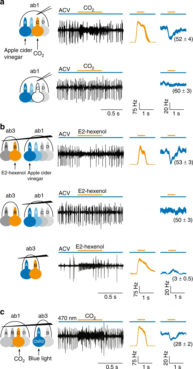
Fig. 1
Direct electrical interaction drives lateral inhibition between ORNs. a The sustained response of ab1A and ab1B was cross-inhibited by the transient activation of ab1C. Top: ab1A/B responded (large sp...
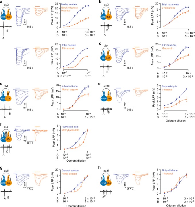
Fig. 2
Comparison of the field responses of grouped neurons. a u2013 f Doseu2212response relationships of grouped ORNs that have distinct extracellular spike amplitudes. a Left: Spontaneous activity of ab2A ...
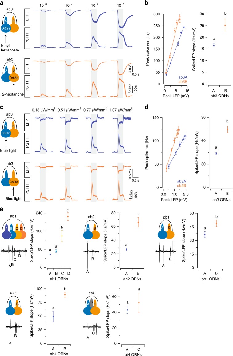
Fig. 3
Comparison of the spiking properties of grouped neurons. a ab3 ORNs were selectively activated by their respective private odorants. a Average LFP responses and the corresponding spike responses are s...
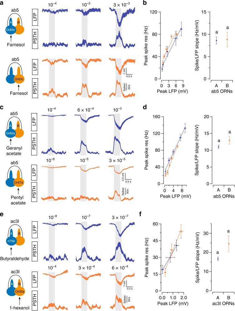
Fig. 4
Spike-LFP analysis in grouped ORNs of similar spike amplitudes. a , b Or83c was ectopically expressed in either ab5A or ab5B using the GAL4-UAS system. ORNs were selectively activated by the odorant, ...
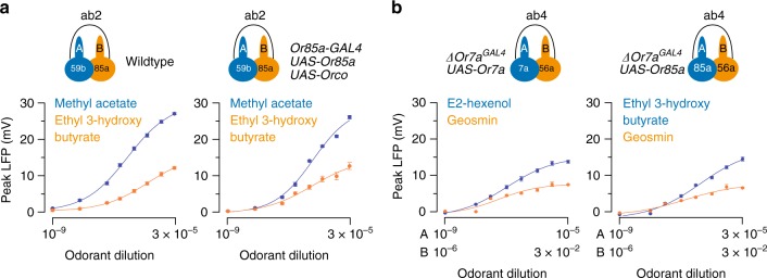
Fig. 5
Overexpressing or swapping odorant receptors does not change the maximal LFP responses of an ORN. a Receptor overexpression in the ab2B ORNs. ab2A responded to methyl acetate and ab2B to ethyl 3-hydro...
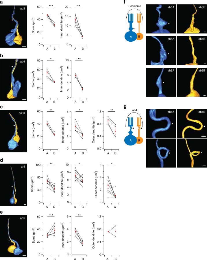
Fig. 6
Systematic morphometric analysis of grouped ORNs. a u2013 e Volumes of the soma, inner and outer dendrites of the paired ORNs in five sensillum types. (Left) Sample 3D reconstruction based on SBEM ima...
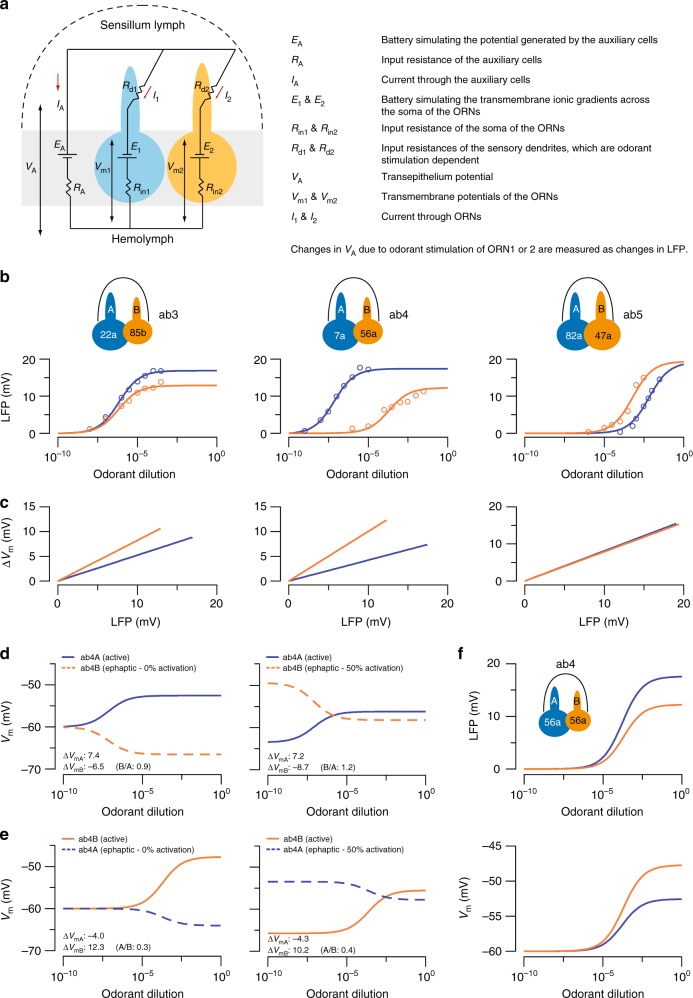
Fig. 7
An electric circuit model for compartmentalized ORNs. a Passive electric circuit model of a sensillum consisting of two ORNs and an auxiliary cell (gray rectangle). b Simultaneous fitting of the LFP r...
Figure images are served from the NIH/NLM PubMed Central Open Access Subset or Europe PMC; copyright remains with the publishers and authors.
💬 Discussion
0 commentsNo comments yet. Be the first to start a discussion!
Leave a Comment