Abstract
AbstractDense reconstruction of synaptic connectivity requires high-resolution electron microscopy images of entire brains and tools to efficiently trace neuronal wires across the volume. To generate such a resource, we sectioned and imaged a larval zebrafish brain by serial block-face electron microscopy at a voxel size of 14 × 14 × 25 nm3. We segmented the resulting dataset with the flood-filling network algorithm, automated the detection of chemical synapses and validated the results by comparisons to transmission electron microscopic images and light-microscopic reconstructions. Neurons and their connections are stored in the form of a queryable and expandable digital address book. We reconstructed a network of 208 neurons involved in visual motion processing, most of them located in the pretectum, which had been functionally characterized in the same specimen by two-photon calcium imaging. Moreover, we mapped all 407 presynaptic and postsynaptic partners of two superficial interneurons in the tectum. The resource developed here serves as a foundation for synaptic-resolution circuit analyses in the zebrafish nervous system.
🔬 Techniques
🧬 Organisms
💻 Software
✨ Fluorophores
🧪 Sample Preparation
🏭 Microscope Brands
🧪 Reagent Suppliers
🔴 Lasers
💻 Software Details
💻 Code & Software
Aligner for large scale serial section image data
PyKNOSSOS is a software tool for the visualization and annotation of 3D image data and was developed for high-throughput image...
Marching Cubes & Mesh Simplification on multi-label 3D images.
💾 Data Repositories
🏛️ Research Organizations (ROR)
Affiliated research institutions:
📋 Methods
Animal husbandry
All animal procedures conformed to the guidelines of the Max Planck Society and the Regierung Oberbayern (protocol number 55.2-1-54-2532-101-12). 2P Ca 2+ imaging We performed Ca 2+ imaging in Tg(elavl3:GCaMP5G)a4598 zebrafish larvae expressing GCaMP5G in almost all neurons at 5 dpf. A few hours before imaging, we fed the larvae paramecia and used only those that consumed paramecia for subsequent imaging. Before imaging, we paralyzed larvae by injecting α-bungarotoxin intraspinally (2 mg ml −1 alpha-bungarotoxin (Invitrogen, B1601), FastRed 10% v/v, 1× Danieau’s solution). We used a movable objective microscope (Sutter Instruments) with a Ti:sapphire (Ti:Sa) laser (Chameleon Ultra II, Coherent) to record GCaMP signals (920 nm; roughly 10 mW after the objective) with a ×20 objective (Olympus, numerical aperture 1.0) and used ScanImage software 53 for image acquisition. We presented visual stimuli to the fish using a custom-built red LED arena (four flat panels covering 360° around the fish; no grating presentation in 30° in front of the fish corresponding to the binocular field). The visual stimulus consisted of vertically oriented gratings moving horizontally in eight phases (gratings in motion for 6 s at spatial frequency of 0.033 cycles per degree and temporal frequency of 2 cycles per s, interspersed with 4 s stationary gratings). Four of the eight phases were monocular, and four were binocular: (1) left nasalward, (2) left temporalward, (3) right temporalward, (4) right nasalward, (5) backward, (6) forward, (7) clockwise and (8) counterclockwise. The sequence of eight phases repeated three times. We recorded a volume centered around the pretectum with roughly 15 z -planes separated by 5 µm. The videos in each z -plane had a size of 512 × 512 pixels (pixel size of 0.385 µm) at a frame rate of 1.74 Hz. Analysis of 2P Ca 2+ -imaging data We processed GCaMP5G signals with a custom-made routine written in MATLAB 25 . Briefly, we focused on 11 most frequent response types in the pretectum and generated a map of correlated pixels for each corresponding regressor. From these regressor maps, we drew regions of interest to detect correlated cells. We cross-checked each of the identified cells with all the regressor maps for overlap. If the same cell was detected in multiple regressor maps, we assigned it the regressor that gave the highest correlation coefficient value. EM sample preparation After 2P microscopy, we anesthetized the animal in 0.016% tricaine in Ringer solution modified for extracellular space preservation (63 mM NaCl, 63 mM cesium gluconate, 2.5 mM KCl, 25 mM NaHCO 3 , 1.25 mM NaH 2 PO 4 , 25 mM glucose, 2 mM CaCl 2 and 1 mM MgCl 2 ) 17 , based on the principle of extracellular space preservation by cell-impermeable solutes 54 . We removed the eyes with a piece of lasso-shaped tungsten wire and removed the skin covering the brain dorsally by first making a small incision caudal and dorsal of the brain using the electrochemically etched tip of a tungsten wire and then, through this incision, inserting the tungsten wire tip under the skin and carefully pulling upward and rostrally, pulling away the skin without touching the brain. We carefully removed any remaining skin flaps with forceps. Finally, we chemically fixed the larva with 2% glutaraldehyde and stained it with the reduced osmium/thiocarbohydrazide/osmium stain, aqueous uranyl acetate and lead aspartate 8 . To make the sample sufficiently conductive to allow imaging even the superficial, plastic-adjacent areas of the brain, we dispersed Carbon Black (2.5% w/v, Ketjenblack, AkzoNobel) in the epoxy 55 .
Show full methods section
Animal husbandry
All animal procedures conformed to the guidelines of the Max Planck Society and the Regierung Oberbayern (protocol number 55.2-1-54-2532-101-12). 2P Ca 2+ imaging We performed Ca 2+ imaging in Tg(elavl3:GCaMP5G)a4598 zebrafish larvae expressing GCaMP5G in almost all neurons at 5 dpf. A few hours before imaging, we fed the larvae paramecia and used only those that consumed paramecia for subsequent imaging. Before imaging, we paralyzed larvae by injecting α-bungarotoxin intraspinally (2 mg ml −1 alpha-bungarotoxin (Invitrogen, B1601), FastRed 10% v/v, 1× Danieau’s solution). We used a movable objective microscope (Sutter Instruments) with a Ti:sapphire (Ti:Sa) laser (Chameleon Ultra II, Coherent) to record GCaMP signals (920 nm; roughly 10 mW after the objective) with a ×20 objective (Olympus, numerical aperture 1.0) and used ScanImage software 53 for image acquisition. We presented visual stimuli to the fish using a custom-built red LED arena (four flat panels covering 360° around the fish; no grating presentation in 30° in front of the fish corresponding to the binocular field). The visual stimulus consisted of vertically oriented gratings moving horizontally in eight phases (gratings in motion for 6 s at spatial frequency of 0.033 cycles per degree and temporal frequency of 2 cycles per s, interspersed with 4 s stationary gratings). Four of the eight phases were monocular, and four were binocular: (1) left nasalward, (2) left temporalward, (3) right temporalward, (4) right nasalward, (5) backward, (6) forward, (7) clockwise and (8) counterclockwise. The sequence of eight phases repeated three times. We recorded a volume centered around the pretectum with roughly 15 z -planes separated by 5 µm. The videos in each z -plane had a size of 512 × 512 pixels (pixel size of 0.385 µm) at a frame rate of 1.74 Hz. Analysis of 2P Ca 2+ -imaging data We processed GCaMP5G signals with a custom-made routine written in MATLAB 25 . Briefly, we focused on 11 most frequent response types in the pretectum and generated a map of correlated pixels for each corresponding regressor. From these regressor maps, we drew regions of interest to detect correlated cells. We cross-checked each of the identified cells with all the regressor maps for overlap. If the same cell was detected in multiple regressor maps, we assigned it the regressor that gave the highest correlation coefficient value. EM sample preparation After 2P microscopy, we anesthetized the animal in 0.016% tricaine in Ringer solution modified for extracellular space preservation (63 mM NaCl, 63 mM cesium gluconate, 2.5 mM KCl, 25 mM NaHCO 3 , 1.25 mM NaH 2 PO 4 , 25 mM glucose, 2 mM CaCl 2 and 1 mM MgCl 2 ) 17 , based on the principle of extracellular space preservation by cell-impermeable solutes 54 . We removed the eyes with a piece of lasso-shaped tungsten wire and removed the skin covering the brain dorsally by first making a small incision caudal and dorsal of the brain using the electrochemically etched tip of a tungsten wire and then, through this incision, inserting the tungsten wire tip under the skin and carefully pulling upward and rostrally, pulling away the skin without touching the brain. We carefully removed any remaining skin flaps with forceps. Finally, we chemically fixed the larva with 2% glutaraldehyde and stained it with the reduced osmium/thiocarbohydrazide/osmium stain, aqueous uranyl acetate and lead aspartate 8 . To make the sample sufficiently conductive to allow imaging even the superficial, plastic-adjacent areas of the brain, we dispersed Carbon Black (2.5% w/v, Ketjenblack, AkzoNobel) in the epoxy 55 .
SBEM data acquisition
We embedded the sample using a custom-designed mold and holder that held the sample in a reproducible position and orientation (Extended Data Fig. 9 ). We then performed X-ray micro-CT imaging of the sample embedded onto the custom holder at 4 µm voxel edge length (SCANCO Medical AG). To generate the EM tile mosaic, we manually segmented the brain tissue in the micro-CT dataset and fit a transformation from the micro-CT coordinate system into that of the SBEM microtome stage motors. By performing dynamic, precomputed X-ray targeted tiling, only 58% of the cuboid bounding box of the brain was scanned. We performed SBEM acquisition on a Zeiss Ultra Plus scanning electron microscope equipped with a Fibics scan generator. Piezo scanning was used, that is the SBEM stage was smoothly moved along the long axis of the scan, while the electron beam scanned the short axis. This resulted in a tile pattern consisting of elongated images (ranging from 4,615 to 25,000 pixels in length, with an average of 16,206 pixels) stacked horizontally, covering the entire brain with the exception of the retinae (Fig. 1d,e ). The ability to extend the FOV to cover the entire brain along one axis reduced the number of FOV positioning moves from 1.3 × 10 6 to 235,581, saving 46 days in ringdown time, similar to the method described previously 56 . In addition to the piezo-scanned image tiles, a single, low-resolution (200 × 200 nm 2 ) overview image was captured per slice with usual electron beam scanning. The microscope was operated by scripted control of the Zeiss SmartSEM v.5 and Fibics ATLAS v.4 software. We used a GV10x downstream asher (ibss Group, Inc.) to clear the detector diode every 2–3 days. To ensure that no sections were lost due to potential thermic shifts in sample position caused by the asher, we retracted and reapproached the sample every time the downstream asher was activated. To map the individual image tiles into a single, consistent 3D space, we used the Aligner package 57 ( https://github.com/billkarsh/Alignment_Projects ), which optimizes an affine transformation for each image tile. To allow for greater flexibility in the alignment, we cut the individual image tiles into shorter pieces of 500 pixels, with 44 pixels overlap, in length along the piezo-scanned ( y ) axis before registration. Alignment of vEM and 2P image stacks To unambiguously match corresponding neurons between the EM and 2P stacks, we devised the sequential transformation steps as follows. First, we manually identified unique landmark points that were visible in both stacks, such as blood vessel branch points, which we subsequently used for calculating transformations using the BigWarp plugin in Fiji 58 . We identified a total of 1,623 corresponding points representing individual somata in the region where the imaged optic-flow responsive cells were located. We divided the pretectal region into smaller regions (‘blocks’) of size 42 × 28 × 2 pixels and the transformation for each block was calculated separately, based on corresponding points located in a surround of that block. Such local affine transformations were calculated for and applied to 3,426 individual blocks on the left side and 3,676 blocks on the right side of the brain. Manual neuron reconstruction and synapse identification Professional annotators of the neuron reconstruction service ariadne.ai ag ( https://www.ariadne.ai ) manually reconstructed the neurons and annotated the synapses. Starting from seed points in somata, the annotators reconstructed the skeleton of the neurons by following their neurites within the 3D EM volume using the open-source neuron reconstruction tools Knossos 33 ( https://knossos.app ) and PyKNOSSOS 13 ( https://github.com/adwanner/PyKNOSSOS ). The annotators manually identified and tagged neurite branch points to revisit and extend them at a later point. We generated consensus skeletons from 3–5 independent reconstructions 13 . The annotators labeled synapses manually using PyKNOSSOS in ‘flight’ mode 13 , where the EM data are displayed in a virtual reslice perpendicular to the local direction of the neurite. They followed the skeletonized axon of every neuron along precalculated paths and annotated all output synapses as described previously 11 . In brief, a synapse was inferred when (1) axonal and dendritic neurite membrane surfaces were parallel and directly apposed, (2) a vesicle cloud was seen in the axon with vesicles in close proximity to the axonal membrane opposite of the dendrite and (3) a thickening or darkening, potentially very faint, of the postsynaptic neurite membrane was observed. In addition, the annotators assigned a subjective confidence level to each synapse. Two independent human annotators performed synapse annotation. If the postsynaptic partner was among the reconstructed cells, this was labeled as such. If a synapse location was found by only one of the two independent annotators, a third expert annotator (F.S.) made the final decision. We measured neurite diameters in the set of skeletonized cells by randomly sampling 200 locations from axons and dendrites each, and keeping fragments of the skeleton within a radius of 750 nm around these locations. The fragments were loaded into PyKNOSSOS and displayed in ‘flight’ mode, allowing a local measurement of the neurite diameter. Morphological characterization of pretectal neurons We compared the targeting of anatomical areas between simple and complex pretectal cells by counting for every cell the number of branch points intersecting one of the region annotations from the light-level atlas registered to our EM dataset. We used branch points instead of all skeleton points to not count parts of the axons and dendrites that only pass through a region. We normalized the branch point counts to the total number of branch points in each category.
Synapse size measurement
We measured synapse sizes in our SBEM dataset by taking a random sample of 100 synaptic contact locations automatically detected in each one of AF6, optic tectum, thalamus and ventral hindbrain, as defined by the mapzebrain region annotations mapped to the SBEM dataset. We manually reviewed these 400 locations to make sure that they precisely represented exactly one synaptic contact and corrected them if necessary. We then calculated contact areas from surface meshes of those contact annotations generated by the zmesh python library ( https://github.com/seung-lab/zmesh ). To enable a comparison to data derived from single two-dimensional (2D) sections, we sliced the 3D contact area objects along each one of the three cardinal directions, spaced by the resolution of the dataset and measured the length of the 2D profile exposed in each section. For high-resolution synapse size measurement, we used a single 35-nm slice of a sample prepared identically to the one used for our SBEM dataset, which we imaged on a JEOL JEM-1230 transmission electron microscope, equipped with a Gatan Orius SC1000 digital camera, at 12,000-fold magnification (pixel size 4.1 × 4.1 nm 2 ) at 80 kV. We measured synaptic contact lengths by sampling 1.5 × 1.5 µm 2 subregions of the tectal neuropil randomly and annotating all intersecting synaptic contacts, until 100 synapses had been measured. Registration to standard brain We trained a 2D U-Net 59 to distinguish soma and neuropil regions in the vEM dataset (Fig. 3b ). In parallel, we obtained a soma and neuropil map in the standard brain coordinate system by thresholding and summing the elavl3:H2B-GCaMP6s (for cell nuclei) and the elavl3:lynTag-RFP (for neuropil) reference brain channels (Fig. 3a ). This allowed us to calculate a diffeomorphic transformation to map these two datasets using the dipy 60 ( https://dipy.org/ ) registration toolkit, which compensates for the complex deformations that the sample underwent during EM preparation.
Tissue classification
Tissue classification models 1 and 2 used the architecture and training hyperparameters described in previous work 22 . Model 1 operated on 28 × 28 × 25 nm 3 data and was trained on manually annotated labels of neuropil (35 megavoxels, MVx), soma (13 MVx) and a class containing blood vessels and ventricles (4 MVx). Model 2 operated on 56 × 56 × 100 nm 3 data and was trained on manually annotated labels of neuropil (114 MVx) and nonneuropil (33 MVx). The annotations for both networks were made independently. Model 3 operated on 56 × 56 × 100 nm 3 data and was trained on binary labels of nucleus (20 MVx) versus not-nucleus (15 MVx). The network architecture was a stack of 16 3D valid-mode convolutions with 32 feature maps, ReLU activation and additive skip connections around every two convolutions, with the exception of the first two. The output of the convolution stack was processed by a point-wise convolution with two feature maps representing the class logits. We trained this network using cross-entropy loss with asynchronous stochastic gradient descent at a learning rate of 10 −3 , batch size of 16 and eight NVIDIA V100 workers. Examples were sampled with equal frequency from every class during training. We binarized the results of model 3, set any voxels predicted as ‘nonneuropil’ or ‘soma’ by model 1 or 2 to 0, and computed the 3D connected components of the results to form an initial soma segmentation. We then applied morphological erosion with radius of 5 to reduce false mergers, and recomputed the 3D connected components. Objects with a volume of more than 1,000 pixels (corresponding to the volume of a sphere with a radius of around 700 nm) were retained as automatically detected soma candidates. We detected defocused regions by filtering the in-plane CLAHE-normalized images with a Gaussian with sigma of 1, followed by a discrete Laplacian filter. For every voxel, we computed the standard deviation of the filtered image within a 21 × 21 region centered at that voxel. We downsampled the results 128× in-plane with area-averaging, and labeled voxels with values
📊 Figures

Fig. 1
Pretectal 2P calcium imaging and whole-brain larval SBEM dataset acquisition.
a , Illustrative larval zebrafish head at 5u2009dpf, brain highlighted in red. b , Wire-frame representation of a 5u2009dpf zebrafish brain, slice stack represents location of the 2P calcium imaged vo...
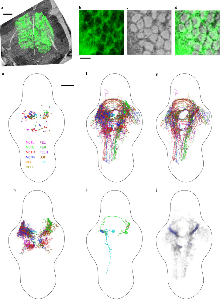
Fig. 2
Mapping and EM-based reconstruction of functionally characterized pretectal neurons.
a , Single plane of GCaMP5G fluorescence registered to SBEM dataset. b u2013 d , Zoomed view of data in a , showing GCaMP5G ( b ) and scanning EM image ( c ) individually and as overlay ( d ). e u2013...
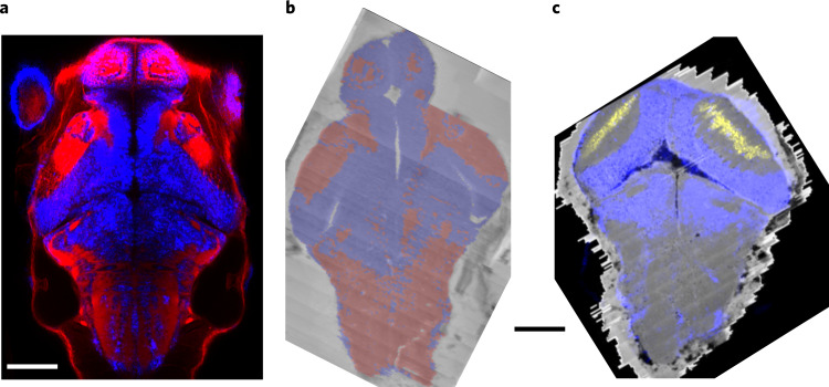
Fig. 3
Registration of LM atlas dataset and vEM stack.
a , elavl3:lynTag-RFP (red) and elavl3:H2B-GCaMP6s (false-colored in blue) fluorescence stacks, registered into a common coordinate system. Dorsal view. b , Soma (blue) and neuropil (red) prediction o...

Fig. 4
Automated neurite segmentation.
a , Dorsal view of the vEM dataset with a multicolored overlay of the base segmentation. b , Close-up examples (one out of at least ten) of the segmentation in, from top left to bottom right, the tect...

Fig. 5
Reconstruction of a SIN and its partners.
a , Dorsal view of the selected SIN1. Input (blue) and output (green) synapses are indicated. b , Annotated (upper panel) and raw data (lower panel) for closely neighboring input (blue) and output (gr...
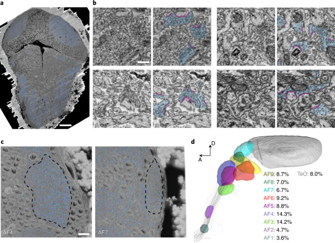
Fig. 6
Automatic detection of synaptic contacts.
a , Dorsal view of the vEM dataset, vesicle clouds labeled in blue. b , Close-up examples of automatically segmented vesicle clouds (blue) and synaptic clefts (magenta) in thalamus (Th), pretectum (pr...
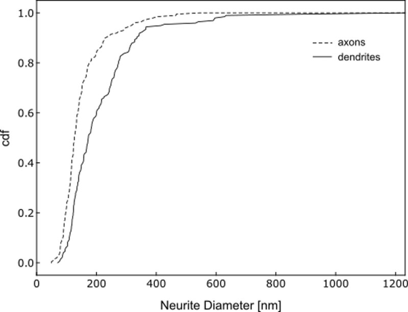
Extended Data Fig. 1
Neurite diameter distribution.
Neurite diameter distribution for pretectal cells (cumulative density function, cdf), measured perpendicular to the main neurite axis in axons and dendrites, at 200 randomly sampled locations in each.

Extended Data Fig. 2
Between-hemisphere comparison of reconstructed pretectal cell morphology.
Fraction of skeleton branch points, taken over all cells, present in different anatomical areas for dendrites of simple (MoNL, MoNR, MoTL and MoTR) and complex (FEL, FER, BEL, BER, FELR, FSP and BSP) ...
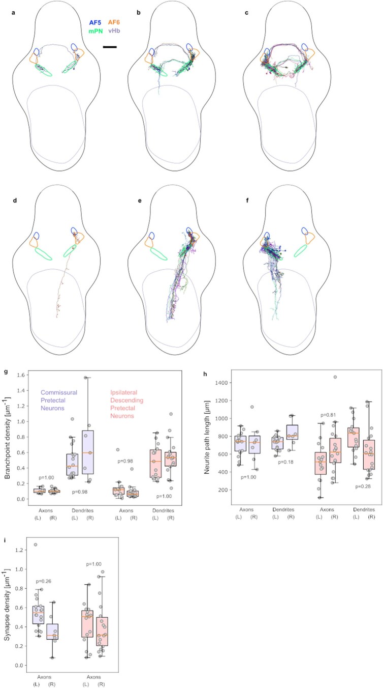
Extended Data Fig. 3
Bilaterally symmetric reconstructions of two morphologically defined pretectal cell types.
Individual example of a commissural pretectal interneuron ( a ) and all neurons of this type with somata on the right ( b ) and left ( c ) side of the brain. d - f . Like a-c , for ipsilateral descend...
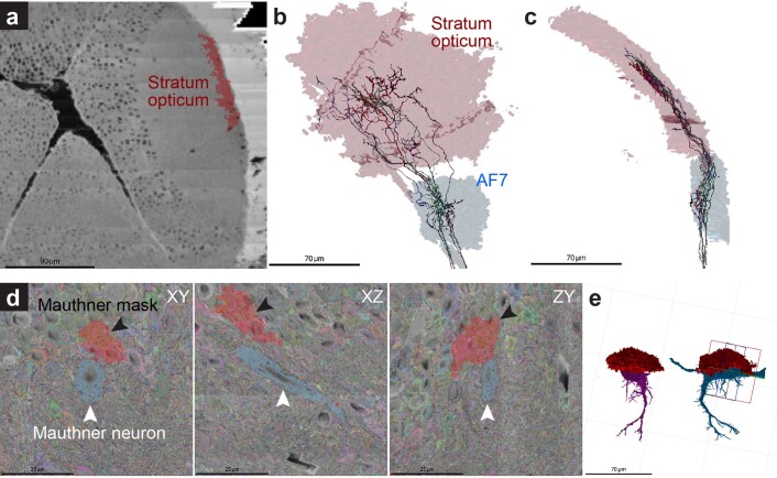
Extended Data Fig. 4
LM-to-EM registration match precision.
Examples for the accuracy of registrations. a - c : Retinal ganglion cell axons (nu2009=u20097), which have been traced in the EM dataset and which project both to the tectal stratum opticum (SO) and ...
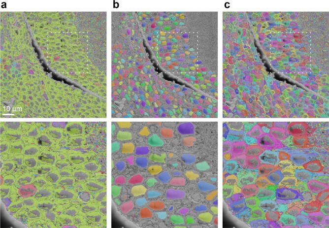
Extended Data Fig. 5
Splitting of merged somata with nuclei segmentation.
a . Initial segmentation with prolific soma-soma mergers, b . Nucleus segmentation, c . Initial segmentation split with nucleus segmentation in ( b ).
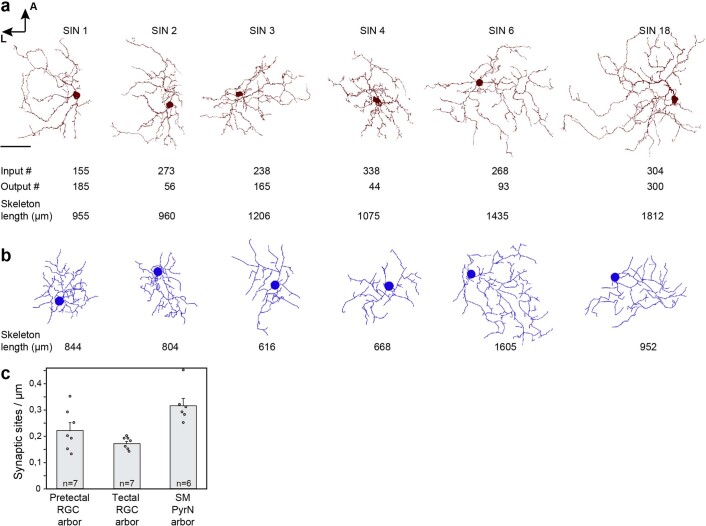
Extended Data Fig. 6
Synapse density and neurite path length comparisons between LM and EM.
a - b . Comparison of reconstructed SINs from our EM dataset ( a ) and from our LM mapzebrain atlas ( b ). The number of input and output synapses is shown below each cell in ( a ) and the neurite pat...
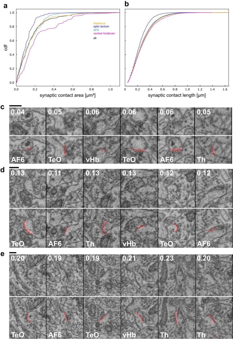
Extended Data Fig. 7
Size of synaptic contacts.
a . Distribution of synaptic contact areas in different brain areas (nu2009=u2009100 in each area). b . For the same synaptic contacts as in a, distribution of contact lengths as exposed in each inter...
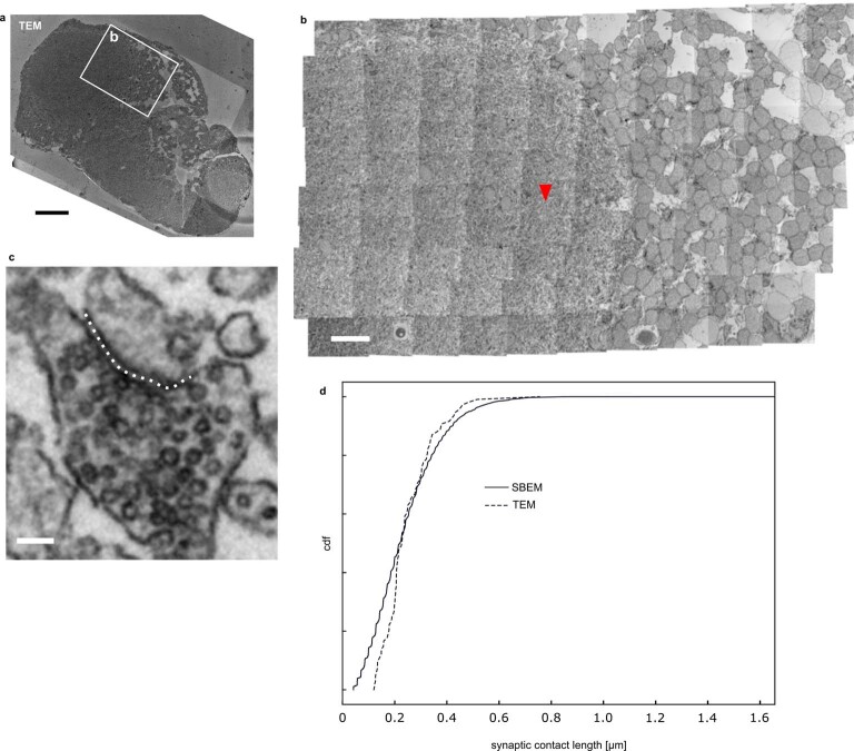
Extended Data Fig. 8
Comparison of synaptic contact lengths in TEM image of optic tectum.
a . Overview of 35u2009nm section of a 5 dpf larval zebrafish prepared identically to the sample used for SBEM. b . Close-up tile mosaic in optic tectum neuropil. Arrowhead points at synapse in ( c )....
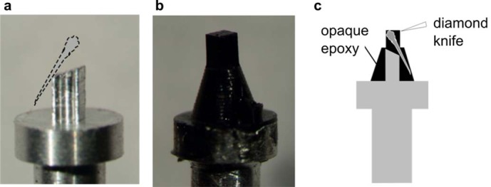
Extended Data Fig. 9
Custom sample holder for reproducible larval zebrafish positioning.
a . Aluminum stub for fish embedding, b . Carbon black epoxy, including fish, cast on the sample holder, c . Schematic cross-section.
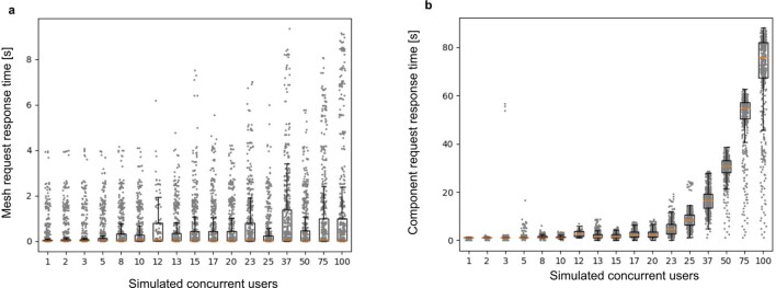
Extended Data Fig. 10
Simulation of proofreading server performance under different concurrent user loads.
a . Response time to request of meshes for cells (either complete or currently undergoing proofreading) and ( b ) to the request of agglomeration graph connected component containing a given supervoxe...
Figure images are served from the NIH/NLM PubMed Central Open Access Subset or Europe PMC; copyright remains with the publishers and authors.
💬 Discussion
0 commentsNo comments yet. Be the first to start a discussion!
Leave a Comment