Abstract
Animals can learn causal relationships between pairs of stimuli separated in time and this ability depends on the hippocampus. Such learning is believed to emerge from alterations in network connectivity, but large-scale connectivity is difficult to measure directly, especially during learning. Here, we show that area CA1 cells converge to time-locked firing sequences that bridge the two stimuli paired during training, and this phenomenon is coupled to a reorganization of network correlations. Using two-photon calcium imaging of mouse hippocampal neurons we find that co-time-tuned neurons exhibit enhanced spontaneous activity correlations that increase just prior to learning. While time-tuned cells are not spatially organized, spontaneously correlated cells do fall into distinct spatial clusters that change as a result of learning. We propose that the spatial re-organization of correlation clusters reflects global network connectivity changes that are responsible for the emergence of the sequentially-timed activity of cell-groups underlying the learned behavior. DOI: http://dx.doi.org/10.7554/eLife.01982.001.
🔬 Techniques
✨ Fluorophores
🧪 Sample Preparation
🏭 Microscope Brands
🧪 Reagent Suppliers
🔴 Lasers
📷 Detectors
💻 Software Details
📋 Protocols
💻 Code & Software
💾 Data Repositories
🏛️ Research Organizations (ROR)
Affiliated research institutions:
📋 Methods
Mice and surgical procedure
All experimental procedures were approved by the National Centre for Biological Sciences Institutional Animal Ethics Committee (Protocol number USB–19–1/2011), in accordance with the guidelines of the Government of India (animal facility CPCSEA registration number 109/1999/CPCSEA) and equivalent guidelines of the Society for Neuroscience. All recordings and behavioral experiments were carried out on male, 30 to 45 day old C57BL/6 mice. Data acquired from a total of 35 mice is included here. A total of 18 mice were trace conditioned, and 17 mice pseudo-conditioned. Of the 18 trace conditioned mice, 9 learned the task to criterion and the other 9 failed to learn. Imaging data was acquired for 14 of the trace conditioned mice. Of these, 6 were learners and 8 were non-learners. Of the 17 pseudo-conditioned mice, imaging data was acquired for 6 mice ( Figure 2—figure supplement 1B ).
Surgical Procedure
Surgery was carried out on a mouse anaesthetized using isoflurane (Abbott, North Chicago, IL, USA) gas anesthesia (3% induction dose and 2% initial maintenance dose (in 95% O 2 , 5%CO 2 ), gradually reduced over a ∼3 hr long procedure). Temperature was maintained using a heating-pad (TR-200, Fine Science Tools, Canada). Dexamethasone 5 mg/kg body weight was injected sub-cutaneously to minimize swelling and bleeding prior to the surgery. The mouse was then head-fixed (Item 51547; Stoelting, Wood Dale, IL, USA) and a custom designed brass head-bar was affixed to the skull using skull-screws (83,438; Micro-Mark, Berkeley Heights, NJ, USA) and dental acrylic. The dorsal hippocampal surface (ipsi-lateral to the side of tone and air-puff delivery) was exposed through a craniotomy (2.0 mm posterior to bregma, 1.5 mm lateral to the mid-line [ipsi-lateral to the side of stimulus delivery]; diameter ∼ 1–1.5 mm) after gently aspirating away over-lying cortex to expose the external capsule ( Dombeck et al., 2007 ). Exposed brain-matter was constantly irrigated with cortex buffer (CB; in mM: NaCl–125, KCl–5, glucose–10, HEPES–10, CaCl2–2 and MgCl2–2. pH set to 7.35 with NaOH) ( Holtmaat et al., 2005 ). A fluorescent indicator of calcium (O6807; Oregon Green BAPTA-1 AM ester, Molecular Probes - Life Technologies, Grand Island, NY, USA) was bolus loaded by pressure injection into the hippocampus, at a depth of ∼100 µm. Pressure injections were delivered using glass pipettes with tip impedances of 2–3 Mohms and pressure pulses of 5–10 psi for 3 to 5 min (Picospritzer-III, Parker-Hannifin, Cleveland, OH, USA). Dye solution was prepared by solubilizing 50 µg of dye (one vial) in 5 µl of a detergent (P-3000MP; 20% Pluronic acid, Invitrogen - Life Technologies), and then diluting down to 1 µg/µl by adding 45 µl of CB. The gap left behind by aspirated cortex was then filled by pouring molten, low-melting agarose solution (A9414; 5% in CB, Sigma, St. Louis, MO, USA) into the craniotomy and covering with a 5 mm, circular cover-slip (CS-5R; Warner Instruments, Hamden, CT, USA). The cover-slip was then fixed in place with dental acrylic. A fragment from a freshly shattered Neodymium magnet was affixed to the left, upper-eyelid using cyano-acrylate glue. Dexamethasone (5 (± 2) µg/g body weight) was injected sub-cutaneously to minimize swelling and bleeding at the beginning of the surgery. Fortwin (Pentazoncine, 5 µg/g body weight) was administered sub-cutaneously at the end of the surgery, as an analgesic. The mouse was then released and given 95% O 2 to breathe until vigorous toe-pinch responses were seen and was then transferred to a closed cage with food and water for 1.5–2 hr, to recover before imaging began. OGB-1 dye, once loaded into neurons, allows imaging for a limited period before clearance from neurons ( Stosiek et al., 2003 ). This limited the viability of the imaging preparation to a few hours, corresponding to a single behavioral session. Behavioral training 1.5 to 2 hr after recovery from anesthesia, mice were head-fixed on a custom-designed clamp (gift from the Albeanu Lab, Cold Spring Habor Laboratory, New York, NY, USA) and mounted onto the stage of a custom-built, two-photon microscope. Left eyelid blink responses were recorded using a custom-made magnetometer ( Koekkoek et al., 2002 ) positioned close to (1–3 mm away) the neodymium magnet fragment glued to the eyelid and was left un-disturbed throughout the experiment. The magnetometer was constructed using a magneto-resistive sensor (HMC1051Z; Honeywell, Linden, NJ, USA), whose output was further amplified (SR560; Stanford Research Systems) and digitized at 10 KHz using a data acquisition card (PCI-6221; National Instruments, Austin, TX, USA). The tone, conditioned stimulus was delivered using a speaker positioned to the left of the mouse. The stimulus was a pure tone of frequency 9.5 KHz, delivered at an intensity of 80–90 dB at the microscope stage and of 350 ms duration. In a pre-training session, only tones were delivered for 30 trials. Blink responses were acquired for 5 s prior to tone onset and terminated 10 s after tone onset. The inter-trial interval was randomized between 15 and 30 s, making the total duration between tone-presentations 30 to 45 s. Thereafter, a single trace conditioning session of 50 trials was carried out. On training trials a 100 ms air-puff (aversive, un-conditioned stimulus), was delivered 250 ms (trace interval) after the end of the tone. Pressurized air at 5 psi was passed through a nozzle of tip-diameter 1–1.5 mm positioned ∼1–2 cm away and aimed at the mouse’s left eye. Air-flow was switched on and off with a computer-controlled electronic, solenoid valve (EV mouse valve, Clippard, Cinncinati, OH, USA). Every fifth trial was a probe trial (on which no puff was delivered) however as these amounted to only 10 probe trials per mouse, data from these trials have not been used for any specific analysis. Only one training session of 50 trials was carried out per mouse. Longer sessions were seen to cause blinking fatigue and discomfort to the mice. Additional sessions over multiple days were not possible due to the acute nature of the imaging preparation (‘Materials and methods: Mice and surgical procedure’). All trained mice were imaged, irrespective of usability of imaging data, while training was carried out. Microscope scan-mirrors continued to oscillate during the inter-trial interval, to remove auditory cues signaling the beginning or end of a trial. Awake, two photon calcium imaging of area CA1 cells Hippocampal area CA1 cells were imaged in parallel with eye-blink acquisition and training. We used a custom-built two-photon microscope, built around a Tsunami, Ti-Sapphire, 80 MHz pulsed laser (Spectra Physics, Mountain View, CA, USA) tuned to 810 nm for excitation with a water dipping objective lens (5CFI75 LWD 16x, NA 0.8, Nikon, Japan). Emitted fluorescent light was detected using an analog GaAsP PMT (H7422P-40; Hamamatsu, Japan). The amplified signal was binned over 2 µs pixel times. Imaging and training were carried out in complete darkness.
Show full methods section
Mice and surgical procedure
All experimental procedures were approved by the National Centre for Biological Sciences Institutional Animal Ethics Committee (Protocol number USB–19–1/2011), in accordance with the guidelines of the Government of India (animal facility CPCSEA registration number 109/1999/CPCSEA) and equivalent guidelines of the Society for Neuroscience. All recordings and behavioral experiments were carried out on male, 30 to 45 day old C57BL/6 mice. Data acquired from a total of 35 mice is included here. A total of 18 mice were trace conditioned, and 17 mice pseudo-conditioned. Of the 18 trace conditioned mice, 9 learned the task to criterion and the other 9 failed to learn. Imaging data was acquired for 14 of the trace conditioned mice. Of these, 6 were learners and 8 were non-learners. Of the 17 pseudo-conditioned mice, imaging data was acquired for 6 mice ( Figure 2—figure supplement 1B ).
Surgical Procedure
Surgery was carried out on a mouse anaesthetized using isoflurane (Abbott, North Chicago, IL, USA) gas anesthesia (3% induction dose and 2% initial maintenance dose (in 95% O 2 , 5%CO 2 ), gradually reduced over a ∼3 hr long procedure). Temperature was maintained using a heating-pad (TR-200, Fine Science Tools, Canada). Dexamethasone 5 mg/kg body weight was injected sub-cutaneously to minimize swelling and bleeding prior to the surgery. The mouse was then head-fixed (Item 51547; Stoelting, Wood Dale, IL, USA) and a custom designed brass head-bar was affixed to the skull using skull-screws (83,438; Micro-Mark, Berkeley Heights, NJ, USA) and dental acrylic. The dorsal hippocampal surface (ipsi-lateral to the side of tone and air-puff delivery) was exposed through a craniotomy (2.0 mm posterior to bregma, 1.5 mm lateral to the mid-line [ipsi-lateral to the side of stimulus delivery]; diameter ∼ 1–1.5 mm) after gently aspirating away over-lying cortex to expose the external capsule ( Dombeck et al., 2007 ). Exposed brain-matter was constantly irrigated with cortex buffer (CB; in mM: NaCl–125, KCl–5, glucose–10, HEPES–10, CaCl2–2 and MgCl2–2. pH set to 7.35 with NaOH) ( Holtmaat et al., 2005 ). A fluorescent indicator of calcium (O6807; Oregon Green BAPTA-1 AM ester, Molecular Probes - Life Technologies, Grand Island, NY, USA) was bolus loaded by pressure injection into the hippocampus, at a depth of ∼100 µm. Pressure injections were delivered using glass pipettes with tip impedances of 2–3 Mohms and pressure pulses of 5–10 psi for 3 to 5 min (Picospritzer-III, Parker-Hannifin, Cleveland, OH, USA). Dye solution was prepared by solubilizing 50 µg of dye (one vial) in 5 µl of a detergent (P-3000MP; 20% Pluronic acid, Invitrogen - Life Technologies), and then diluting down to 1 µg/µl by adding 45 µl of CB. The gap left behind by aspirated cortex was then filled by pouring molten, low-melting agarose solution (A9414; 5% in CB, Sigma, St. Louis, MO, USA) into the craniotomy and covering with a 5 mm, circular cover-slip (CS-5R; Warner Instruments, Hamden, CT, USA). The cover-slip was then fixed in place with dental acrylic. A fragment from a freshly shattered Neodymium magnet was affixed to the left, upper-eyelid using cyano-acrylate glue. Dexamethasone (5 (± 2) µg/g body weight) was injected sub-cutaneously to minimize swelling and bleeding at the beginning of the surgery. Fortwin (Pentazoncine, 5 µg/g body weight) was administered sub-cutaneously at the end of the surgery, as an analgesic. The mouse was then released and given 95% O 2 to breathe until vigorous toe-pinch responses were seen and was then transferred to a closed cage with food and water for 1.5–2 hr, to recover before imaging began. OGB-1 dye, once loaded into neurons, allows imaging for a limited period before clearance from neurons ( Stosiek et al., 2003 ). This limited the viability of the imaging preparation to a few hours, corresponding to a single behavioral session. Behavioral training 1.5 to 2 hr after recovery from anesthesia, mice were head-fixed on a custom-designed clamp (gift from the Albeanu Lab, Cold Spring Habor Laboratory, New York, NY, USA) and mounted onto the stage of a custom-built, two-photon microscope. Left eyelid blink responses were recorded using a custom-made magnetometer ( Koekkoek et al., 2002 ) positioned close to (1–3 mm away) the neodymium magnet fragment glued to the eyelid and was left un-disturbed throughout the experiment. The magnetometer was constructed using a magneto-resistive sensor (HMC1051Z; Honeywell, Linden, NJ, USA), whose output was further amplified (SR560; Stanford Research Systems) and digitized at 10 KHz using a data acquisition card (PCI-6221; National Instruments, Austin, TX, USA). The tone, conditioned stimulus was delivered using a speaker positioned to the left of the mouse. The stimulus was a pure tone of frequency 9.5 KHz, delivered at an intensity of 80–90 dB at the microscope stage and of 350 ms duration. In a pre-training session, only tones were delivered for 30 trials. Blink responses were acquired for 5 s prior to tone onset and terminated 10 s after tone onset. The inter-trial interval was randomized between 15 and 30 s, making the total duration between tone-presentations 30 to 45 s. Thereafter, a single trace conditioning session of 50 trials was carried out. On training trials a 100 ms air-puff (aversive, un-conditioned stimulus), was delivered 250 ms (trace interval) after the end of the tone. Pressurized air at 5 psi was passed through a nozzle of tip-diameter 1–1.5 mm positioned ∼1–2 cm away and aimed at the mouse’s left eye. Air-flow was switched on and off with a computer-controlled electronic, solenoid valve (EV mouse valve, Clippard, Cinncinati, OH, USA). Every fifth trial was a probe trial (on which no puff was delivered) however as these amounted to only 10 probe trials per mouse, data from these trials have not been used for any specific analysis. Only one training session of 50 trials was carried out per mouse. Longer sessions were seen to cause blinking fatigue and discomfort to the mice. Additional sessions over multiple days were not possible due to the acute nature of the imaging preparation (‘Materials and methods: Mice and surgical procedure’). All trained mice were imaged, irrespective of usability of imaging data, while training was carried out. Microscope scan-mirrors continued to oscillate during the inter-trial interval, to remove auditory cues signaling the beginning or end of a trial. Awake, two photon calcium imaging of area CA1 cells Hippocampal area CA1 cells were imaged in parallel with eye-blink acquisition and training. We used a custom-built two-photon microscope, built around a Tsunami, Ti-Sapphire, 80 MHz pulsed laser (Spectra Physics, Mountain View, CA, USA) tuned to 810 nm for excitation with a water dipping objective lens (5CFI75 LWD 16x, NA 0.8, Nikon, Japan). Emitted fluorescent light was detected using an analog GaAsP PMT (H7422P-40; Hamamatsu, Japan). The amplified signal was binned over 2 µs pixel times. Imaging and training were carried out in complete darkness.
Data analysis
All analysis was carried out using custom-written programs (Matlab, Mathworks, Natick, MA, USA), unless otherwise mentioned. Matlab code for the behavioral learning curves analysis ( Wirth et al., 2003 ; Smith et al., 2004 ) and meta k-means analysis ( Ozden et al., 2008 ; Dombeck et al., 2009 ) is available with the authors of the studies to first use it. Code for the main analyses carried out for this study is available for download at https://github.com/mehrabmodi/CA1-sequences-data-analysis-code.git .
Behavioral analysis
Magnetometer trace baseline was calculated as the median of values recorded in a 2.4 s time window just prior to tone stimulus delivery. The entire trace was baseline-subtracted using this value. Blink response to tone was calculated by summing data values acquired from tone onset to air-puff onset (600 ms in total). Significant or conditioned blink responses (CR) were identified using a threshold given by, (1) threshold = µ ( blink pre ) + 2σ ( blink pre ) where blink pre is the area under the pre-training blink response curves in the time interval between tone onset and puff onset. Using this threshold, each trial was classified as either a blink (1) or a non-blink (0) trial, yielding a binary response vector for each mouse. CRs were identified in a 600 ms time-window after tone onset. Hence, the probability of blink responses by chance was calculated as below. (2) p chance = 1 / ( n time windows ) = 0.11 Here, p chance is the probability of a well-timed CR by chance and n time windows is the number of 600 ms time windows before puff onset (5600/600 = 9.33). We then used a previously described expectation maximization algorithm to calculate learning curves for each mouse, as well as the learning trial if the mouse was identified as a learner ( Smith et al., 2004 ). For the purposes of analysis, the mean ‘learning-trial’ across trained learners was assigned to all pseudo-conditioned mice. As an independent analysis of behavioral performance, we also calculated a performance score (PS) for each mouse. PS was defined as the ratio of CR frequency to spontaneous blink frequency. For the identification of spontaneous blinks, four 600 ms time-windows (2400 ms totally) before tone onset were considered. The same criterion for significant blinks was applied to these time windows and the fraction of windows (4 × 50 = 200 total windows) containing significant blinks was calculated as the spontaneous blink fraction.
Image analysis
An averaged image from the first five frames of the first trial was used to manually draw regions of interest (ROIs) around cell-bodies. An averaged image from the first five frames of each trial was then used as a reference image for that trial. Each frame in the trial was aligned to this reference image using the TurboReg plugin for ImageJ ( Thevenaz et al., 1998 ) to correct for movement of the imaged field during the trial. This registration method does not correct for within-frame motion. For each frame, cell intensity was calculated as the mean intensity of pixels within its ROI. Normalized, background-subtracted ΔF/F traces were calculated from these according to the equation, (3) ( Δ F F ) i = F i F b a s e l i n e − 1 where F i is cell fluorescence on frame- i and F baseline is the median fluorescence intensity of the cell on that trial. Only 4 s of data around the time of tone delivery were considered for this analysis, wherein the baseline was considered to be stable. Two metrics of cell activity during a 4 s long, spontaneous activity period (5 s away from any stimulus) were used to test for stability of imaging datasets. The summed area under the curve and the number of peaks detected were both calculated for the first and last 25% of trials. Datasets from mice showing statistically significant differences (two sample t test, p4 s away from tone or puff delivery from each considered trial. The traces for a cell were stitched together for groups of trials and correlation coefficients were calculated for each pair of these, extended traces. In this way, noise correlations were computed for all appropriate cell pairs in each dataset. Trial-groups were considered as described in Figure 4A, and 6A,B . Note that for most analyses involving spontaneous activity correlations, cells were not discarded on the basis of their reliability scores as in the case of time-tuning analyses. The only exception is the analysis for Figure 4—figure supplement 1B . Here, neurons were classified into two groups, one with high activity timing reliability scores, and the other with low activity timing reliability scores. Spontaneous activity correlations were then calculated for pairs of neurons within each group that shared the same activity peak timing.
Clustering analysis
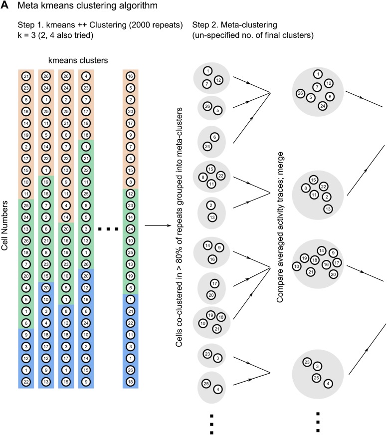
Meta k-means was employed to sort neurons into groups, so as to maximize within group correlations while minimizing across group correlations ( Ozden et al., 2008 ). Briefly, the k means ++ algorithm ( Arthur and Vassilvitskii, 2007 ) was initialized with k = 3 and was run 2000 times to generate clusters, after which cell-pairs falling into the same k-means ++ cluster for >80% of iterations were placed into ‘meta-clusters’. We also initialized k-means ++ with k = 2 and k = 4, and similar results were obtained. These meta-clusters were then iteratively combined using pair-wise correlation coefficient as a criterion, as described previously ( Dombeck et al., 2009 ) to yield the final clusters. Since the final clusters are formed by iterative pooling of meta-clusters, the number of clusters does not need to be pre-specified. The number of clusters obtained ranged from 2 to 8, while the k-value used to initialize k-means ++ in the reported data was 3. Grouping or cluster similarity score The cluster similarity score was calculated for pairs of cell correlation clusters, with an aim to characterize how similar the two clusters were. First, the proportion of neurons belonging in common to both clusters was calculated, followed by calculating the overlap seen by chance, when random neurons were assigned to equal sized clusters. This is because overlap expected by chance depends on the numbers and sizes of clusters. The ratio of these two overlap measures was defined as the similarity score. In order to match clusters across trial sets, all possible combinations of cluster pairing in the two datasets were considered, and the one with the highest overlap proportion was used to calculate the similarity scores.
Statistical testing with multiple comparisons
When making comparisons between more than two samples, we used the Tukey-Kramer honest significant difference test in conjunction with a one-way analysis of variance. The test calculates 99% confidence intervals around the mean of each sample, and reports significant differences between any pair of samples if the intervals do not overlap. The calculation of intervals accounts for the increased chances of type-1 errors due to multiple comparisons. Since 99% confidence intervals were calculated, the chance of error is smaller than 1%. Hence, p values were reported as
📊 Figures
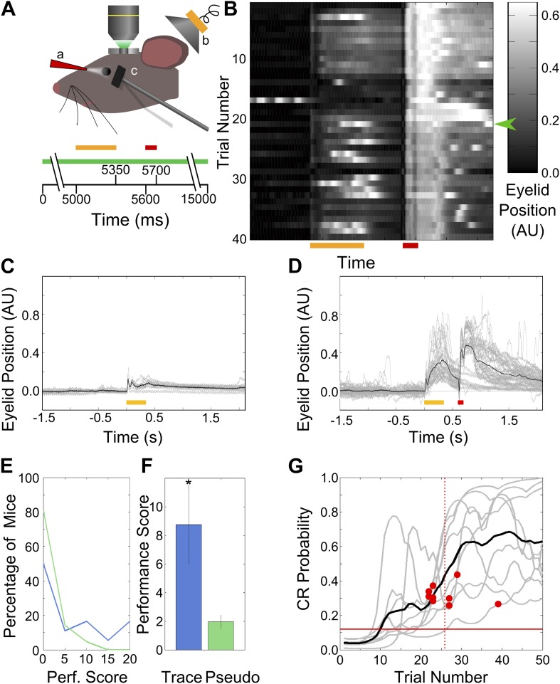
Figure 1.
Behavior: trace eye-blink conditioning of mice.
( A ) Cartoon schematic of experimental system. Two-photon calcium imaging was carried out in area CA1 of the dorsal hippocampus in a head-fixed mouse which underwent trace eyeblink conditioning. A sp...
Video 1.
Mouse Behavior.
Video of mouse eyeblink behavior acquired at 100 frames per second (fps) and played back at 10 fps (i.e. 0.1x speed). A yellow spot in the bottom-right corner indicates when tone is being delivered, a...
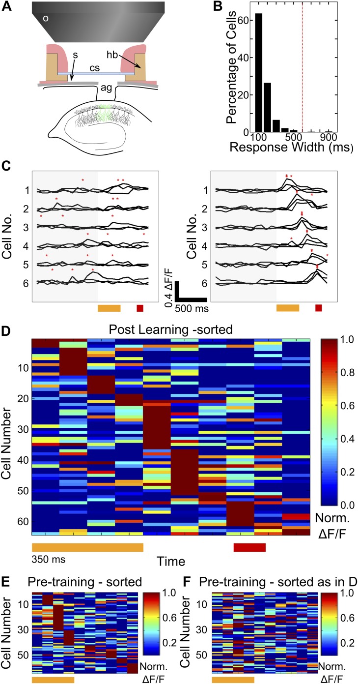
Figure 2.
Two-photon imaging of calcium-responses in area CA1 neurons from awake mice.
( A ) Schematic of the imaging preparation. ou2013objective lens, su2013skull, csu2013cover slip, hbu2013head bar, agu2013agarose. ( B ) Histogram of neuron response widths in ms, calculated as the ti...
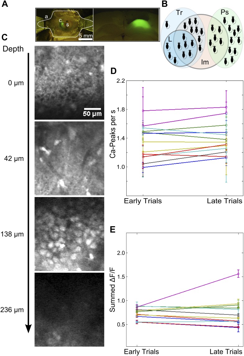
Figure 2u2014figure supplement 1.
Imaging preparation and calcium response data.
( A ) Left: Top-view of a head-fixed, awake mouse. a: white outline of custom-designed head bar affixed to the dorsal surface of the skull using skull-screws and dental acrylic. s: exposed skull. c: c...
Video 2.
Calcium responses.
Video showing a time-series of images of a single field of view of area CA1 cells. Brighter colors in the gray-scale indicate higher fluorescence intensities. Flashes visible are calcium responses. DO...
Video 3.
z-stack of dye-loaded hippocampal tissue.
Video showing optical sections through a typical, dye-loaded imaging preparation of the dorsal hippocampus. Optical sections were acquired beginning at the dorsal hippocampal surface and moving ventra...
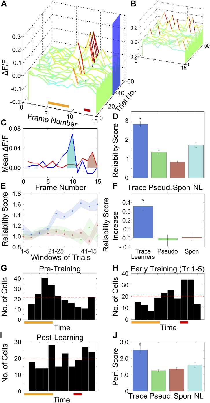
Figure 3.
After training, area CA1 cells show reliably timed, sequential calcium responses.
( A ) Calcium response traces for an example neuron, aligned to the time of stimulus delivery (tone and puff indicated by yellow and red bars at bottom respectively). Warmer colors in the traces indic...
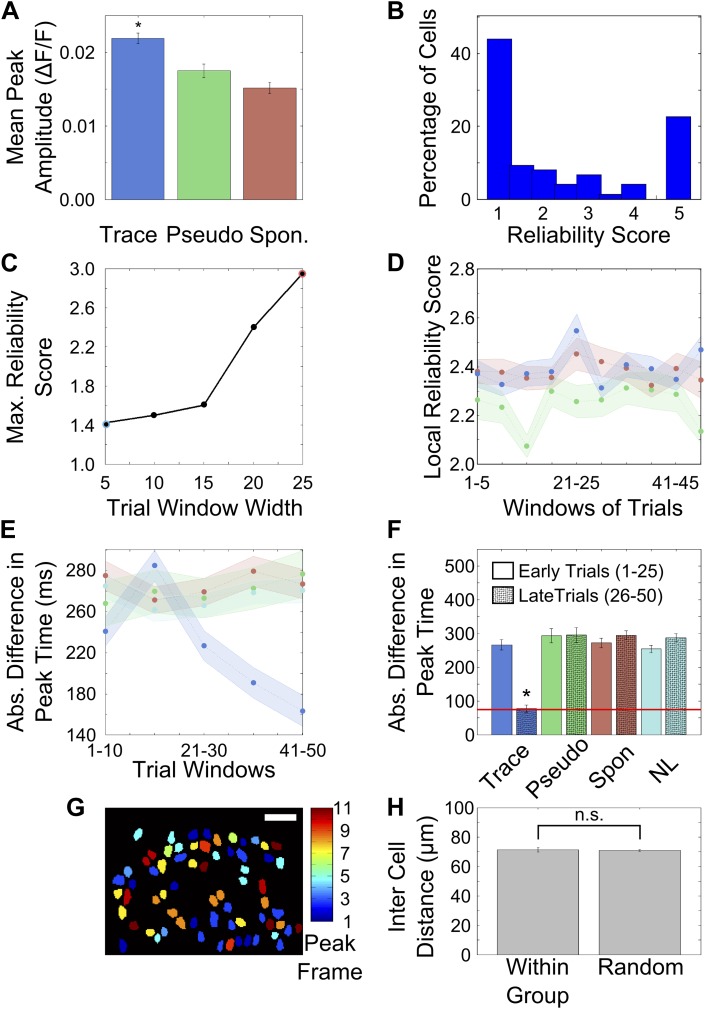
Figure 3u2014figure supplement 1.
Activity peak times change during learning.
( A ) Peak heights in trial-averaged u0394F/F traces are greater for cells from trace conditioned mice than controls. u0394F/F traces from tone onset to air-puff onset were averaged across all trials ...
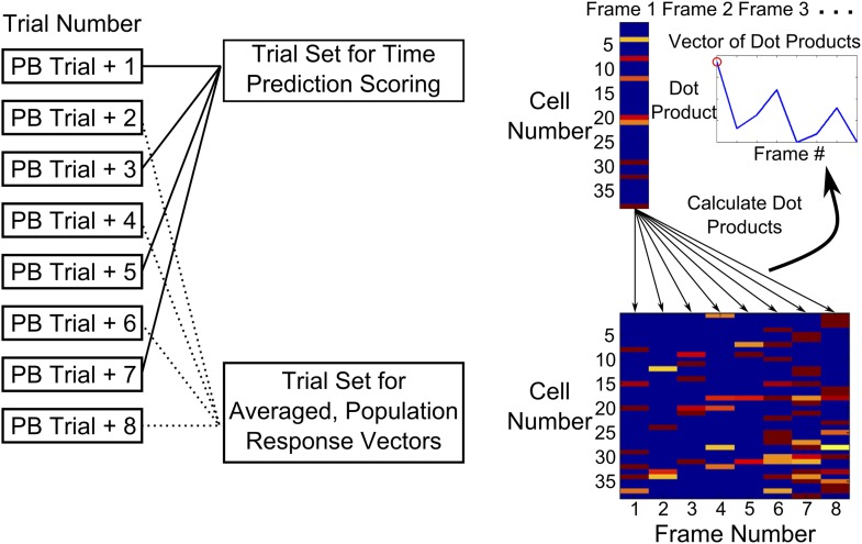
Figure 3u2014figure supplement 2.
Time-decoder algorithm.
Schematic explaining the use of a template matching time decoder. Trials after peak behavioral trial were alternately split into two groupsu2014one training set averaged to obtain a template of expect...
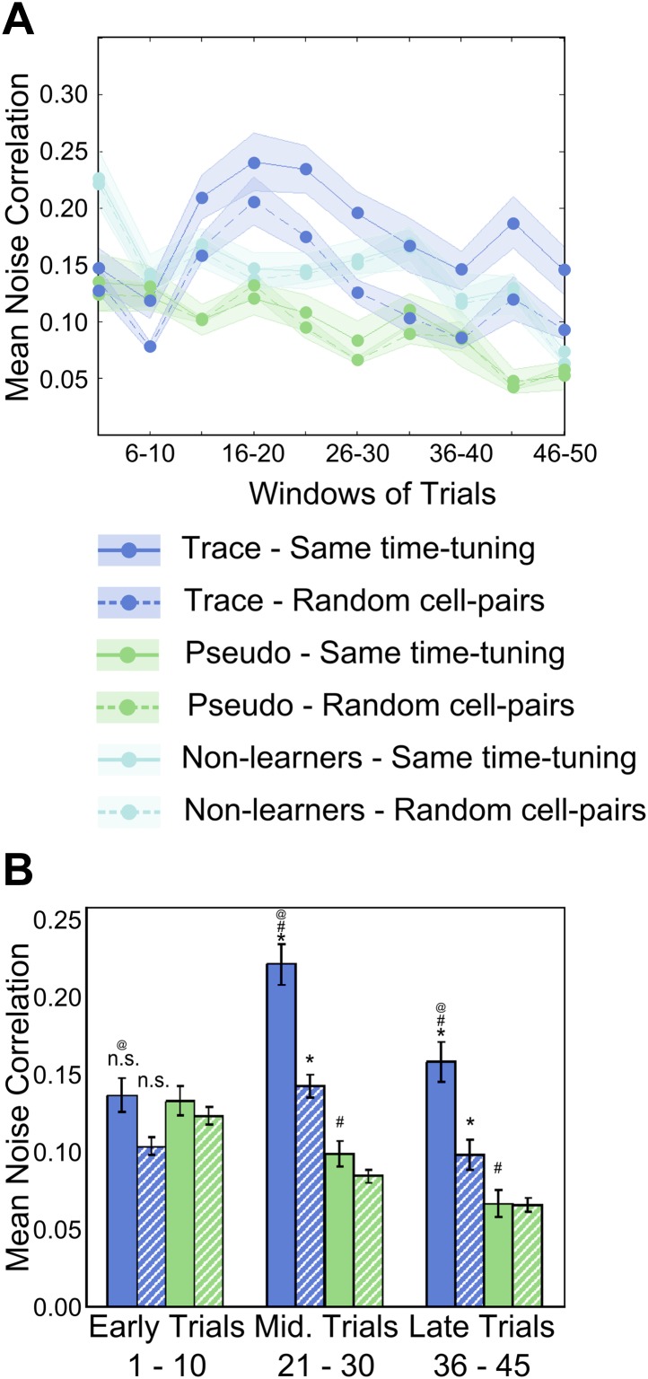
Figure 4.
Area CA1 cell noise-correlations increase transiently during training.
( A ) Average neuron-pair noise correlations plotted as a function of training trials for task learner mice (blue curves), pseudo-conditioned mice (green curves) and non-learners (cyan curves). Solid ...
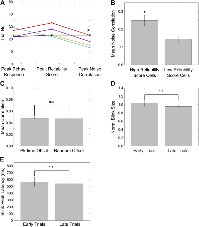
Figure 4u2014figure supplement 1.
Peaks of CR rate curve, CA1 activity timing reliability and NC; characterization of NC changes during learning.
( A ) Plots for individual mice, showing the trial number (or middle of trial-bin) of the training session when the learning trials, peaks in mean reliability scores of time-locked activity and mean s...
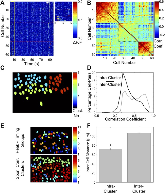
Figure 5.
Correlated neurons are spatially clustered.
( A ) Neurons within clusters show within-group, correlated activity. Spontaneous, u0394F/F calcium activity traces for neurons from an example dataset. Neurons are sorted as per clusters identified b...
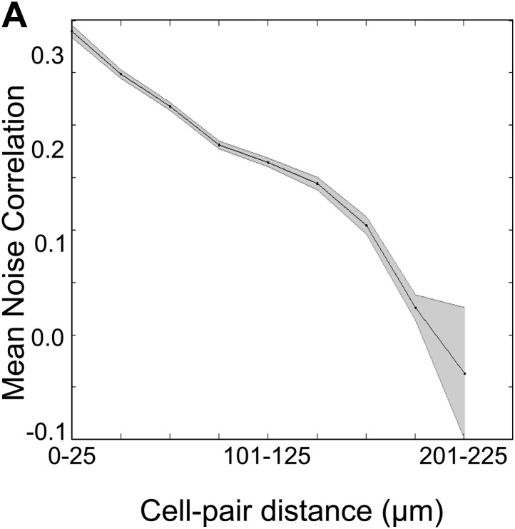
Figure 5u2014figure supplement 1.
Spontaneous activity correlations fall with increasing inter-cell distance.
Mean of the spontaneous activity correlations for all cell-pairs plotted against the binned distances between these cell-pairs. The shaded area represents SEM. Correlation coefficient = u22120.178, p&...
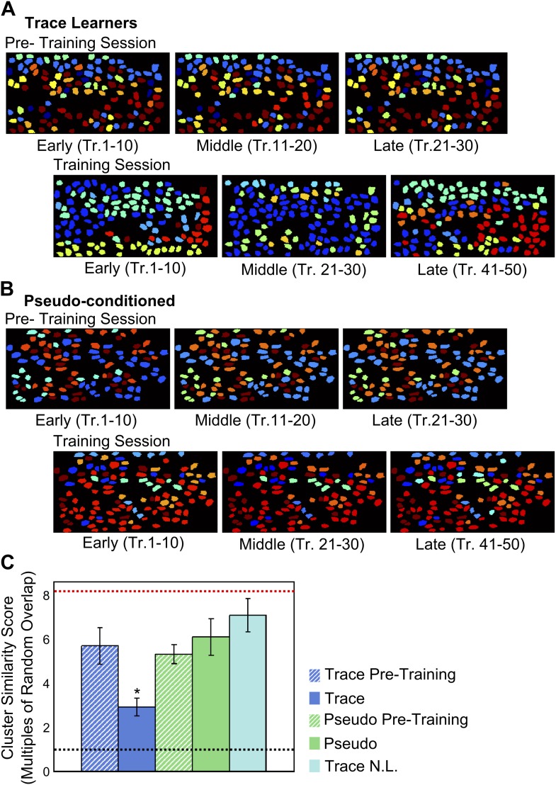
Figure 6.
Correlated neuron-groups are spatially re-distributed during trace conditioning.
( A and B ) Sample trace-conditioned ( A ) and pseudo-conditioned ( B ) mouse neuron-clusters, identified in early (left), middle (center) and late (right) trials, for pre-training (top) as well as tr...
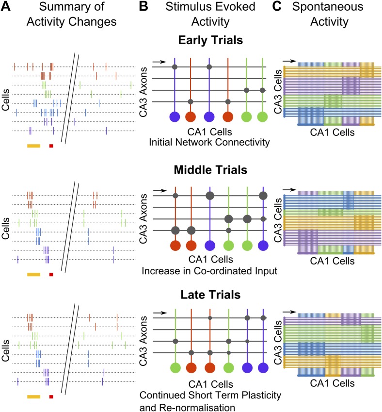
Figure 7.
Summary and model schematics.
( A ) Schematic summarizing findings: early in the session (top), neuron activity peaks are tuned to stimuli. Spontaneous activity is largely un-correlated. By the middle of the session (center), time...
Author response image 1.
Schematic describing how the meta k-means clustering algorithm works.
Author response image 2.
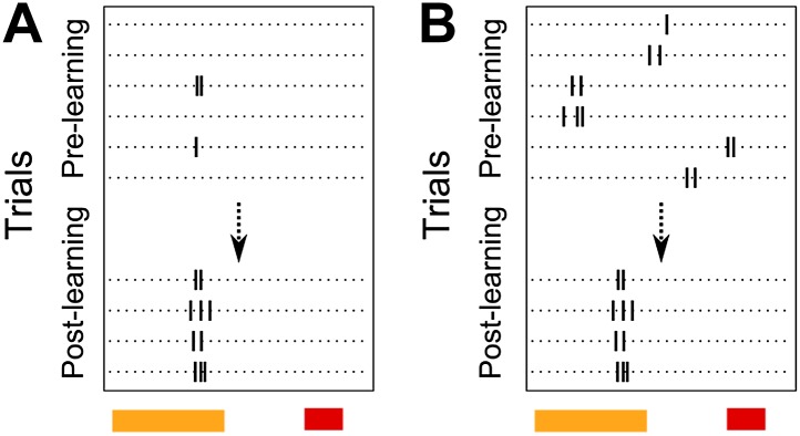
Schematic diagram depicting two possible patterns of learning related changes in timing of activity peaks. A Activity peak timing is fixed from the beginning of the session, only reliability of trial ...
Author response image 3.
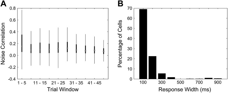
A Mean noise correlations for non-learners are high in the first trial bin. This is not due to the presence of a few outliers. This panel is a box and whisker plot for the noise correlation data corre...
Figure images are served from the NIH/NLM PubMed Central Open Access Subset or Europe PMC; copyright remains with the publishers and authors.
💬 Discussion
0 commentsNo comments yet. Be the first to start a discussion!
Leave a Comment