Abstract
Selective Plane Illumination Microscopy (SPIM) is an imaging technique particularly suited for long term in-vivo analysis of transparent specimens, able to visualize small organs or entire organisms, at cellular and eventually even subcellular resolution. Here we report the application of SPIM in Calcium imaging based on Förster Resonance Energy Transfer (FRET). Transgenic Arabidopsis plants expressing the genetically encoded-FRET-based Ca(2+) probe Cameleon, in the cytosol or nucleus, were used to demonstrate that SPIM enables ratiometric fluorescence imaging at high spatial and temporal resolution, both at tissue and single cell level. The SPIM-FRET technique enabled us to follow nuclear and cytosolic Ca(2+) dynamics in Arabidopsis root tip cells, deep inside the organ, in response to different stimuli. A relevant physiological phenomenon, namely Ca(2+) signal percolation, predicted in previous studies, has been directly visualized.
🔬 Techniques
🔭 Microscopes
🧬 Organisms
💻 Software
✨ Fluorophores
🏭 Microscope Brands
📷 Detectors
💻 Software Details
🏛️ Research Organizations (ROR)
Affiliated research institutions:
📋 Methods
SPIM apparatus The microscope is a modified version of the OpenSPIM project [30] , and it is similar to a single illumination arm SPIM [31] . A single mode fiber coupled laser at 442 nm (MDL-III-442, CNI) is collimated and used for SPIM illumination. An automatic shutter switches the beam on and off via computer control. A cylindrical lens focuses the light in a horizontal plane and a 1× telescope images the focal plane of the cylindrical lens in the back focal plane of the illumination 10× water dipping microscope objective (UMPLFLN 10XW, Olympus). As a result, a vertical light-sheet is created on the sample in the front focal plane of this objective. A slit placed in the center of the telescope confines the excitation light-sheet within the imaged area. The height of the light-sheet is 600 µm and its thickness is about 3 µm (beam waist in the focal plane of the illumination objective). Typical illumination power at the sample was between 10 and 50 µW. We didn't observe any photo-bleaching (during continuous illumination for more than 5 minutes) for illumination powers below 15 µW. The detection unit consists in a 20× water dipping microscope objective (UMPLFLN 20XW, Olympus), a tube lens (U-TLU-1-2, Olympus), and a dual sensor CCD camera (Orca D2, Hamamatsu Photonics K.K.). The illumination and the detection microscope objectives are precisely aligned at 90° in the imaging chamber, which is filled with a water-based solution. The detector consists of a dual-CCD system in which the two sensors are positioned at 90° after a dichroic filter (at 510 nm). One of the two sensors can be rotated and translated to correct focus and alignment in order to produce high contrast images. In addition to the dichroic filter, two band-pass filters (centered at 483 and 542 nm) are used to detect CFP and cpVenus (FRET) signals simultaneously. A white-LED illuminator in transmitted light configuration is used during the alignment of the sample to minimize the exposure to the laser light.
Show full methods section
SPIM apparatus The microscope is a modified version of the OpenSPIM project [30] , and it is similar to a single illumination arm SPIM [31] . A single mode fiber coupled laser at 442 nm (MDL-III-442, CNI) is collimated and used for SPIM illumination. An automatic shutter switches the beam on and off via computer control. A cylindrical lens focuses the light in a horizontal plane and a 1× telescope images the focal plane of the cylindrical lens in the back focal plane of the illumination 10× water dipping microscope objective (UMPLFLN 10XW, Olympus). As a result, a vertical light-sheet is created on the sample in the front focal plane of this objective. A slit placed in the center of the telescope confines the excitation light-sheet within the imaged area. The height of the light-sheet is 600 µm and its thickness is about 3 µm (beam waist in the focal plane of the illumination objective). Typical illumination power at the sample was between 10 and 50 µW. We didn't observe any photo-bleaching (during continuous illumination for more than 5 minutes) for illumination powers below 15 µW. The detection unit consists in a 20× water dipping microscope objective (UMPLFLN 20XW, Olympus), a tube lens (U-TLU-1-2, Olympus), and a dual sensor CCD camera (Orca D2, Hamamatsu Photonics K.K.). The illumination and the detection microscope objectives are precisely aligned at 90° in the imaging chamber, which is filled with a water-based solution. The detector consists of a dual-CCD system in which the two sensors are positioned at 90° after a dichroic filter (at 510 nm). One of the two sensors can be rotated and translated to correct focus and alignment in order to produce high contrast images. In addition to the dichroic filter, two band-pass filters (centered at 483 and 542 nm) are used to detect CFP and cpVenus (FRET) signals simultaneously. A white-LED illuminator in transmitted light configuration is used during the alignment of the sample to minimize the exposure to the laser light.
Sample preparation
The sample consists of 12–14 day-old transgenic Arabidopsis seedlings expressing the cytosolic (NES-YC3.6) or nuclear (NLS-YC3.6) localized Cameleon YC3.6. The generation of these lines was previously reported in Ref. [19] in which the full description of the targeting strategies is reported. The seeds are surface sterilized by vapor-phase sterilization and directly placed, with a toothpick, over a conical plastic holder (typically a 10 µL pipette tip) [32] . The holder is filled with half strength Murashige and Skoog medium (MS, M0222 elements including Vitamins, Duchefa, http://www.duchefa-biochemie.nl/ ) [33] supplemented with 0.1% sucrose, 2.34 mM MES with a final pH of the media to 6.0±0.1 with 0.5 M KOH and 0.8% of micro agar (Duchefa). The plastic holders are then transferred to a transparent plastic box filled with sterile half strength MS solution for hydroponic culture and placed in a growth chamber under 16/8 h cycles of white light at 22°C. The hydroponic system allows the seedling roots to grow, following the positive gravitropism, first into the agar and subsequently directly in hydroponic solution when they reach the bottom hole of the holder. Once the root comes out the hole of the plastic holder, the specimen is transferred to the SPIM-FRET setup into the imaging chamber filled with the desired solution (for our Ca 2+ dynamic analyses a 10 mM MES, 5 mM KCl, 10 mM CaCl 2 , pH 5.8 adjusted with TRIS-BASE solution was employed). This procedure prevents any kind of damage or major stress to the root and maintains the seedling vertical. For the analysis of spatiotemporal dynamics of the [Ca 2+ ] rise, a volume of 120 µL (100X) glutamate (L-Glu) or external ATP (eATP) was directly added to one corner of the imaging chamber (filled with 12 mL of imaging solution). The final concentration of the stimuli was 1 mM and 0.1 mM for L-Glu and eATP respectively. The stock ATP solution was diluted in a TRIS buffer (pH 5.8) in order to prevent any pH change of the imaging solution.
Imaging procedure
In the course of SPIM acquisition the root was imaged simultaneously by the 2 CCDs of the dual-sensor camera (Orca D2, Hamamatsu Photonics K.K.) and automatically translated with steps of 1 to 10 µm to create a 3D reconstruction of a large tissue volume by generating multiple image stacks. The shutter, the translation stage and the camera were controlled using Micro-Manager ( www.micro-manager.org ). This software enables the user to easily program the scanning of the sample over the light sheet and time-lapse acquisition parameters at the beginning of each experiment. The exposure time for each plane was typically 50–500 ms. Two different types of acquisitions were carried out: i) two-dimensional analysis, in which a single plane was imaged with continuous illumination and multiple acquisitions lasting 60–300 s; ii) three-dimensional analysis, in which several planes (typically 10–20) were acquired successively: every 5–10 s the acquisition of the entire stack was repeated. The fluorescence intensity was determined over Regions Of Interests (ROIs) corresponding to large root tip areas, single cells or nuclei. Background subtraction was performed in each channel before FRET ratio calculation by selecting a ROI outside the sample. The FRET ratio (R) was calculated and visualized using the Ratio Plus Plugin for Fiji ( http://fiji.sc/ ) or NisElement (Nikon). For time course experiments the change in the FRET ratio (ΔR) was normalized to the initial value (R 0 ) and plotted versus time (ΔR/R 0 ).
Imaging procedure
In the course of SPIM acquisition the root was imaged simultaneously by the 2 CCDs of the dual-sensor camera (Orca D2, Hamamatsu Photonics K.K.) and automatically translated with steps of 1 to 10 µm to create a 3D reconstruction of a large tissue volume by generating multiple image stacks. The shutter, the translation stage and the camera were controlled using Micro-Manager ( www.micro-manager.org ). This software enables the user to easily program the scanning of the sample over the light sheet and time-lapse acquisition parameters at the beginning of each experiment. The exposure time for each plane was typically 50–500 ms. Two different types of acquisitions were carried out: i) two-dimensional analysis, in which a single plane was imaged with continuous illumination and multiple acquisitions lasting 60–300 s; ii) three-dimensional analysis, in which several planes (typically 10–20) were acquired successively: every 5–10 s the acquisition of the entire stack was repeated. The fluorescence intensity was determined over Regions Of Interests (ROIs) corresponding to large root tip areas, single cells or nuclei. Background subtraction was performed in each channel before FRET ratio calculation by selecting a ROI outside the sample. The FRET ratio (R) was calculated and visualized using the Ratio Plus Plugin for Fiji ( http://fiji.sc/ ) or NisElement (Nikon). For time course experiments the change in the FRET ratio (ΔR) was normalized to the initial value (R 0 ) and plotted versus time (ΔR/R 0 ).
Supporting Information Figure S1 Sagittal (A–C) and two transverse sections (D–I) of the specimen (Arabidopsis expressing the nuclear localized Cameleon) for CFP signal, cpVenus and FRET ratio. The sagittal sections are acquired within approximately one third of the sample thickness. The transverse sections are obtained scanning the entire sample within the light sheet. Scale bar is 50 µm. (TIF) Click here for additional data file. Figure S2 Statistical analysis of the response amplitude and duration, in root tip of Arabidopsis seedlings expressing the nuclear or cytosolic localized Cameleon, for 0.1 mM eATP and 1 mM L-Glu stimuli. (A) Mean value of the FRET ratio changes measured on the peak of the response (ΔR max /R 0 ). (B) Mean value of the FRET ratio changes measured 40 s after the stimulus (ΔR t40 /R 0 ). The eATP response is still active at long times while the L-Glu response is depleted. Values are means ± SE (n = 6). p-values were calculated by Student's t test. (TIF) Click here for additional data file. Figure S3 Comparison of different microscopy modalities for measuring eATP-induced Ca 2+ dynamics in root tip of Arabidopsis seedlings expressing the cytosolic localized Cameleon. Selected FRET ratios images of the root tip at different time points from the sensing (Pre) of the eATP stimulus acquired with: (A) Wide-field microscopy with a 20× detection objective as described in Ref. [20] ; (B) CLSM analysis. The images were acquired with a 63× water immersion objective as described in Ref. [41] ; (C) SPIM microscopy. The images were acquired with a 20× objective as described in Material and methods. Scale bar is 50 µm. Background subtraction was not applied to these experiments. (TIF) Click here for additional data file. Movie S1 Three-dimensional (3D) reconstruction of the primary root tip of Arabidopsis thaliana (CFP fluorescence signal) expressing the nuclear localized Cameleon. (MP4) Click here for additional data file. Movie S2 Three-dimensional (3D) reconstruction of a lateral root primordium of Arabidopsis thaliana (CFP fluorescence signal) expressing the nuclear localized Cameleon. (MP4) Click here for additional data file. Movie S3 Three-dimensional (3D) reconstruction of the root mature zone of Arabidopsis thaliana (CFP fluorescence signal) expressing the nuclear localized Cameleon. (MP4) Click here for additional data file. Movie S4 Time series of nuclear FRET ratio images of an Arabidopsis seedling root tip expressing the nuclear localized Cameleon challenged with 1 mM L-Glu. The movie plays 4 times at real-time. (AVI) Click here for additional data file. Movie S5 Time series of nuclear FRET ratio images of an Arabidopsis seedling root tip expressing the nuclear localized Cameleon challenged with 0.1 mM eATP. The movie plays 4 times at real-time. (AVI) Click here for additional data file. Movie S6 Time series of cytosolic FRET ratio images of an Arabidopsis seedling root tip expressing the cytosolic localized Cameleon challenged with 1 mM L-Glu. The movie plays 4 times at real-time. (AVI) Click here for additional data file. Movie S7 Time series of cytosolic FRET ratio images of an Arabidopsis seedling root tip expressing the cytosolic localized Cameleon challenged with 0.1 mM eATP. The movie plays 4 times at real-time. (AVI) Click here for additional data file. Movie S8 Time lapse 3D reconstruction of nuclear FRET ratio of an Arabidopsis seedling root tip expressing the nuclear localized Cameleon challenged with 0.1 mM eATP. The movie plays 20 times at real-time. (AVI) Click here for additional data file. Movie S9 Time lapse 3D reconstruction of cytosolic FRET ratio of an Arabidopsis seedling root tip expressing the cytosolic localized Cameleon challenged with 0.1 mM eATP. The movie plays 20 times at real-time. (AVI) Click here for additional data file.
📊 Figures
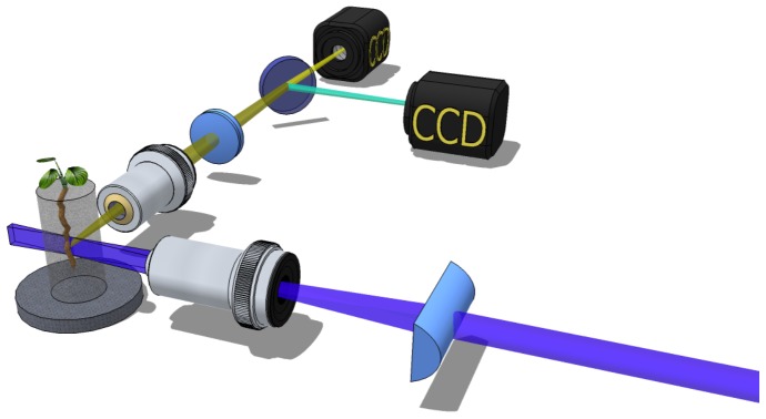
Figure 1
Schematic of the SPIM-FRET setup: a cylindrical lens in combination with a microscope objective create a light-sheet on the sample orthogonal to the detection axis.
Two CCDs are used to image the CFP (Fluorescence) and cpVenus (FRET) signals. Note that for the simultaneous acquisition of the two channels, several configurations are possible: i) two independent ca...
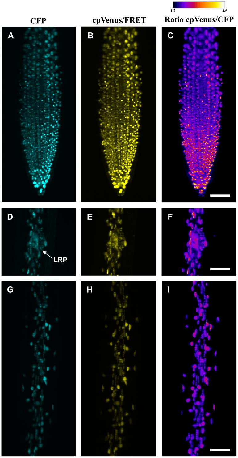
Figure 2
Maximum intensity projections of the stacks obtained for CFP (A,D,G), cpVenus/FRET (B,E,H) and Ratio between the two channels (C,F,I) in different regions of the Arabidopsis thaliana root (primary root tip, lateral root primordium and root mature zone) expressing the nuclear localized Cameleon.
LRP: lateral root primordium. Scale bar is 50 u00b5m.
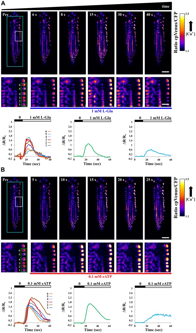
Figure 3
Single plane FRET ratio in root tip of Arabidopsis seedlings expressing the nuclear localized Cameleon, measured at different times in the course of 1-Glu (A) and 0.1 mM eATP (B) stimuli.
(A) First row: FRET ratio images at different time points from the sensing (Pre) of the L-Glu stimulus. Second row: close up (white rectangle in the top-left image) of the FRET ratios including 6 sele...
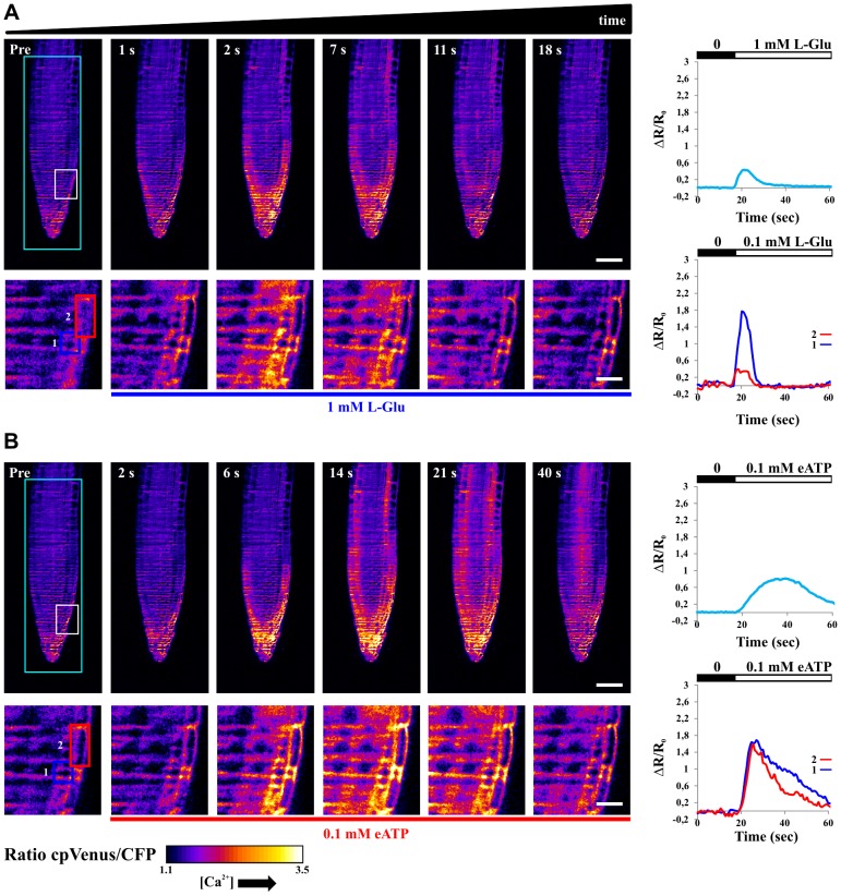
Figure 4
Single plane FRET ratio in root tip of Arabidopsis seedlings expressing the cytosolic localized Cameleon, measured at different times in the course of 1-Glu (A) and 0.1 mM eATP (B) stimuli.
(A) Upper images: FRET ratio measured at different time points from the sensing (Pre) of the L-Glu stimulus. Lower images: close up (white rectangle in the top-let image) of the same selected FRET rat...
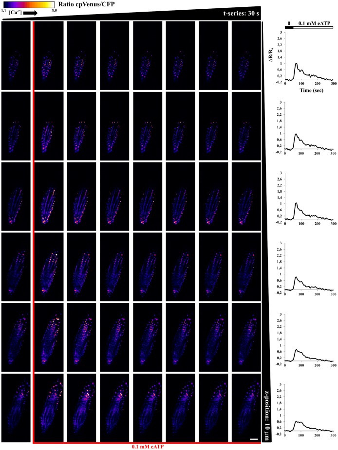
Figure 5
FRET ratio imaged in space and time, with 10 u00b5m steps (columns) and every 30 s (rows), in root tip of Arabidopsis seedlings expressing the nuclear localized Cameleon, in the course of 0.1 mM eATP stimulus.
Graphs on the right hand side show temporal evolution of the averaged FRET ratio for each single selected plane. Scale bar is 50 u00b5m.
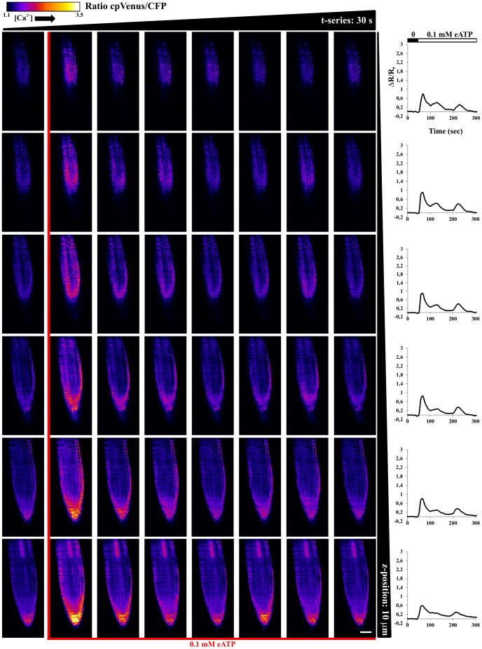
Figure 6
FRET ratio imaged in space and time, with 10 u00b5m steps (columns) and every 30 s (rows), in root tip of Arabidopsis seedlings expressing the cytosolic localized Cameleon, in the course of 0.1 mM eATP stimulus.
Graphs on the right hand side report temporal evolution of the average FRET ratio for each single selected plane. Scale bar is 50 u00b5m.
Figure images are served from the NIH/NLM PubMed Central Open Access Subset or Europe PMC; copyright remains with the publishers and authors.
💬 Discussion
0 commentsNo comments yet. Be the first to start a discussion!
Leave a Comment