Abstract
Brains regulate behavioral responses with distinct timings. Here we investigate the cellular and molecular mechanisms underlying the timing of decision-making during olfactory navigation in Caenorhabditis elegans. We find that, based on subtle changes in odor concentrations, the animals appear to choose the appropriate migratory direction from multiple trials as a form of behavioral decision-making. Through optophysiological, mathematical and genetic analyses of neural activity under virtual odor gradients, we further find that odor concentration information is temporally integrated for a decision by a gradual increase in intracellular calcium concentration ([Ca2+]i), which occurs via L-type voltage-gated calcium channels in a pair of olfactory neurons. In contrast, for a reflex-like behavioral response, [Ca2+]i rapidly increases via multiple types of calcium channels in a pair of nociceptive neurons. Thus, the timing of neuronal responses is determined by cell type-dependent involvement of calcium channels, which may serve as a cellular basis for decision-making.
🔬 Techniques
🧬 Organisms
✨ Fluorophores
🧪 Sample Preparation
🏭 Microscope Brands
📷 Detectors
🎨 Filters
💻 Software Details
📋 Protocols
💾 Data Repositories
🏛️ Research Organizations (ROR)
Affiliated research institutions:
📋 Methods
Strains
The techniques used for culturing and handling C. elegans were essentially as described previously ( Brenner, 1974 ). The C. elegans wild-type Bristol strain N2, RRID: WB-STRAIN:JD21 cca-1(ad1650) , RRID: WB-STRAIN:MT1212 egl-19(n582) , RRID: WB-STRAIN:JT73 itr-1(sa73) , RRID: WB-STRAIN:CX3222 odr-3(n1605) , RRID: WB-STRAIN:CX2205 odr-3(n2150) , RRID: WB-STRAIN:CB55 unc-2(e55) , RRID: WB-STRAIN:MT7929 unc-13(e51) , RRID: WB-STRAIN:DA509 unc-31(e928), and RRID: WB-STRAIN:CB540 unc-68(e540) were obtained from the Caenorhabditis Genetics Center (University of Minnesota, USA). In all the behavioral and physiological experiments, young adult hermaphrodites were used. Multi-worm tracking and analysis of 2-nonanone avoidance on a 9 cm plate Quantitative analysis of the 2-nonanone avoidance of wild-type animals in the 9 cm agar plate was carried out as previously described ( Kimura et al., 2010 ; Yamazoe-Umemoto et al., 2015 ). In brief, several adult animals per assay were transferred to the center of a 9 cm NGM agar plate either directly from a standard 6 cm nematode growth medium (NGM) plate with the food bacteria OP-50 (‘fed’) or after a 1 hr starvation on the NGM plate without OP-50 (‘starved’). In the following analysis, we used a data set that is a mixture of 50 fed and 50 starved animals. Although we did not find a significant difference between fed and starved animals in 2-nonanone avoidance ( Kimura et al., 2010 ), the feeding state (fed or starved) could affect some aspects of C. elegans ' behavior ( Bargmann, 2006 ) and we wanted to focus on feeding state-independent behavioral aspects of the animals. Two μL of 30% 2-nonanone (diluted in EtOH) were put in two spots on the surface of the agar plate ( Figures 1A and 2A ), and images of the animals during the avoidance behavior were captured at 1 Hz for 12 min by our multi-worm tracking system with a high-resolution camera in a fixed position ( Kawazoe et al., 2013 ; Yamazoe-Umemoto et al., 2015 ). In this study, we used a CMOS camera CSB4000F-10 (Toshiba Teli Corp., Japan) equipped with a C mount adaptor and a Nikkor 50 mm f/1.2 lens (Nikon Corp., Japan). Because the camera captures the entire area of the 9 cm plate with a resolution of 2008 × 2044 pixels, an animal of length ~1 mm and width ~0.05 mm is depicted in ~25 pixels. x−y coordinates of the centroids of the animals in each image were measured by Move-tr/2D software (Library Inc., Japan), and were further analysed by Excel2010 (Microsoft) or R (The R Project). Because the animals did not initiate avoidance during the first 2 min on average ( Kimura et al., 2010 ) ( Figures 1A and 2B and Figure 2—figure supplement 1E ), data between 121–720 s were used for the analysis ( Tanimoto et al., 2017 ). Definition of pirouettes and runs A pirouette is a period of frequent turns and migrations whose duration is shorter than a threshold value ( Pierce-Shimomura et al., 1999 ). The animal's behavioral state in one second was classified as a turn if the absolute value of angle change in migratory vector of the animal's centroid from the previous second ( i.e., during 1 s) was larger than 90° or if the migratory velocity was smaller than 0.1 mm/s in the following frames after the large angle change. According to this definition, the reverse and the omega turn ( Gray et al., 2005 ) were recognized as turns. A distribution of turn intervals ( i.e., migratory durations) during 2-nonanone avoidance was well-fitted by a sum of two exponentials for shorter and longer intervals ( Figure 1—figure supplement 1A ). A period at which the numbers of the short and long intervals were equal was 13.1 s and determined as t crit according to the original definition ( Pierce-Shimomura et al., 1999 ). Migrations whose turn interval was longer than t crit were classified as runs, and migrations shorter than t crit as well as turns were classified in pirouettes. Bearings at the initiation of and during runs The directions of animal migrations for 1 s were defined in terms of the bearing, B, with respect to the 2-nonanone gradient, where B = 0° indicates migration directly away from the odor source ( i.e., down the gradient) and B = ±180° indicates migration directly toward the odor source ( i.e., up the gradient). Bearing at run initiation in salt-taxis by the previous study was calculated from the results of taxis toward NH 4 Cl (56.0%) and biotin (55.2%) in Figure 9 of the report ( Pierce-Shimomura et al., 1999 ).
Show full methods section
Strains
The techniques used for culturing and handling C. elegans were essentially as described previously ( Brenner, 1974 ). The C. elegans wild-type Bristol strain N2, RRID: WB-STRAIN:JD21 cca-1(ad1650) , RRID: WB-STRAIN:MT1212 egl-19(n582) , RRID: WB-STRAIN:JT73 itr-1(sa73) , RRID: WB-STRAIN:CX3222 odr-3(n1605) , RRID: WB-STRAIN:CX2205 odr-3(n2150) , RRID: WB-STRAIN:CB55 unc-2(e55) , RRID: WB-STRAIN:MT7929 unc-13(e51) , RRID: WB-STRAIN:DA509 unc-31(e928), and RRID: WB-STRAIN:CB540 unc-68(e540) were obtained from the Caenorhabditis Genetics Center (University of Minnesota, USA). In all the behavioral and physiological experiments, young adult hermaphrodites were used. Multi-worm tracking and analysis of 2-nonanone avoidance on a 9 cm plate Quantitative analysis of the 2-nonanone avoidance of wild-type animals in the 9 cm agar plate was carried out as previously described ( Kimura et al., 2010 ; Yamazoe-Umemoto et al., 2015 ). In brief, several adult animals per assay were transferred to the center of a 9 cm NGM agar plate either directly from a standard 6 cm nematode growth medium (NGM) plate with the food bacteria OP-50 (‘fed’) or after a 1 hr starvation on the NGM plate without OP-50 (‘starved’). In the following analysis, we used a data set that is a mixture of 50 fed and 50 starved animals. Although we did not find a significant difference between fed and starved animals in 2-nonanone avoidance ( Kimura et al., 2010 ), the feeding state (fed or starved) could affect some aspects of C. elegans ' behavior ( Bargmann, 2006 ) and we wanted to focus on feeding state-independent behavioral aspects of the animals. Two μL of 30% 2-nonanone (diluted in EtOH) were put in two spots on the surface of the agar plate ( Figures 1A and 2A ), and images of the animals during the avoidance behavior were captured at 1 Hz for 12 min by our multi-worm tracking system with a high-resolution camera in a fixed position ( Kawazoe et al., 2013 ; Yamazoe-Umemoto et al., 2015 ). In this study, we used a CMOS camera CSB4000F-10 (Toshiba Teli Corp., Japan) equipped with a C mount adaptor and a Nikkor 50 mm f/1.2 lens (Nikon Corp., Japan). Because the camera captures the entire area of the 9 cm plate with a resolution of 2008 × 2044 pixels, an animal of length ~1 mm and width ~0.05 mm is depicted in ~25 pixels. x−y coordinates of the centroids of the animals in each image were measured by Move-tr/2D software (Library Inc., Japan), and were further analysed by Excel2010 (Microsoft) or R (The R Project). Because the animals did not initiate avoidance during the first 2 min on average ( Kimura et al., 2010 ) ( Figures 1A and 2B and Figure 2—figure supplement 1E ), data between 121–720 s were used for the analysis ( Tanimoto et al., 2017 ). Definition of pirouettes and runs A pirouette is a period of frequent turns and migrations whose duration is shorter than a threshold value ( Pierce-Shimomura et al., 1999 ). The animal's behavioral state in one second was classified as a turn if the absolute value of angle change in migratory vector of the animal's centroid from the previous second ( i.e., during 1 s) was larger than 90° or if the migratory velocity was smaller than 0.1 mm/s in the following frames after the large angle change. According to this definition, the reverse and the omega turn ( Gray et al., 2005 ) were recognized as turns. A distribution of turn intervals ( i.e., migratory durations) during 2-nonanone avoidance was well-fitted by a sum of two exponentials for shorter and longer intervals ( Figure 1—figure supplement 1A ). A period at which the numbers of the short and long intervals were equal was 13.1 s and determined as t crit according to the original definition ( Pierce-Shimomura et al., 1999 ). Migrations whose turn interval was longer than t crit were classified as runs, and migrations shorter than t crit as well as turns were classified in pirouettes. Bearings at the initiation of and during runs The directions of animal migrations for 1 s were defined in terms of the bearing, B, with respect to the 2-nonanone gradient, where B = 0° indicates migration directly away from the odor source ( i.e., down the gradient) and B = ±180° indicates migration directly toward the odor source ( i.e., up the gradient). Bearing at run initiation in salt-taxis by the previous study was calculated from the results of taxis toward NH 4 Cl (56.0%) and biotin (55.2%) in Figure 9 of the report ( Pierce-Shimomura et al., 1999 ).
Calibration curve for 2-nonanone measurement
Calibration curve for 2-nonanone measurement is described in more detail at Bio-protocol ( Yamazoe-Umemoto et al., 2018 ). To measure local concentrations of gaseous 2-nonanone in the assay plate, we used a gas chromatograph (GC) with a sensitive semiconductor detector, SGVA-N2, which was optimized for 2-nonanone detection (FIS Inc., Japan). To make a calibration curve for the measurement, 0.36, 1.07, 3.56, 35.6, 59.4, 97.2, and 200 μL of liquid 2-nonanone (Wako Pure Chemical, Japan) were vaporized in a 50 L tank DT-T1 (FIS Inc.), each corresponding to 0.04, 0.12, 0.4, 4.0, 6.8, 11.1, and 22.9 μM in the gas phase, respectively. After the volatilization period, 0.2 mL of the gas was sampled with a 2 mL plastic syringe with a needle from an outlet of the tank and was immediately injected into the GC. The volatilization periods were determined for each amount of the liquid to maximize the 2-nonanone signal. Synthetic air Alphagaz 1 (Air Liquide, Japan) was used as a carrier gas. With 260 s retention time, a single large peak of signal intensity (mV) was detected as 2-nonanone signal ( Figure 2—figure supplement 1B ). The experiments were repeated 3–4 times for each concentration. The correlations between the peak height of the signal and the gaseous 2-nonanone concentration in a log-log plot were well-fitted by two simple regression lines for lower and higher concentrations ( Figure 2—figure supplement 1C ; R 2 >0.999 for both). In general, for semiconductor detectors, the correlation between the peak height of the signal and signal concentration in a log-log plot are well-fitted by two simple regression lines for lower and higher concentrations. Measuring odor gradient by gas chromatograph Measuring odor gradient by gas chromatograph is described in more detail at Bio-protocol ( Yamazoe-Umemoto et al., 2018 ). For the odor sampling, a hole of 1 mm in diameter was made through the bottom of the plastic plate and the agar. Because the molecular weight of 2-nonanone (FW 142.2) is larger as a volatile compound, it did not leak easily from such a small hole. 1, 3, 6, 9 and 12 min after placing the odor at the two spots, a 2 mL plastic syringe, which is the same type as the one used in the calibration, was inserted into the plate through the hole from the bottom, and 0.2 mL of the gas phase was sampled ( Figure 2—figure supplement 1A ). Each plate was used only once to avoid disturbance of the gradient by the sampling. The sampled gas was immediately injected into the GC for measurement. The concentration of 2-nonanone was calculated from the height of the signal peak according to the regression line for the calibration. For each data point, the measurements were repeated 7–9 times and median and quartile was calculated for the fitting. Fitting the odor gradient and calculation of C worm Fitting the odor gradient and calculation of C worm are described in more detail at Bio-protocol ( Yamazoe-Umemoto et al., 2018 ). The least squares method was used to fit the measured concentration. In the closed plate, the odor concentration asymptotically approaches a constant value. Therefore the measured concentrations were fitted to a phenomenological curve with two exponential saturation functions: C(x, y, t ) = a ( r 1 )(1-exp(- b ( r 1 ) t )) + a ( r 2 )(1-exp(- b ( r 2 ) t )). r 1 and r 2 are the distances from the position ( x, y ) on the agar to the two odor sources. The asymptotic concentration a ( r ) and the increasing rate b ( r ) are functions of the distance r such as a ( r )= a 0 exp(- a 1 r - a 2 r 2 ) and b ( r )= b 0 exp(- b 1 r - b 2 r 2 ). The assumption that C ( x, y, t ) is given by the sum of the two independent functions is valid for the low concentration regions x > 0. The fitting parameters a 0 = 20.68 μM, a 1 = 0.7355 cm −1 , a 2 = −0.05408 cm −2 , b 0 = 0.8384 min −1 , b 1 = 0.7835 cm −1 and b 2 = −0.05761 cm −2 were determined by the Levenberg-Marquardt method ( Press et al., 1992 ). We consider the measured and the fitted odor gradient as reliable because it is consistent with the fact that the amount of 2-nonanone at the source was apparently reduced by 20–30% after 12 min and with a theoretically calculated simulation ( Yamazoe-Umemoto et al., 2015 ). The 2-nonanone concentration at a given temporal and spatial point of an animal’s centroid was calculated from the fitting curve and was designated as C worm . Turning rate shown in Figure 2D was determined as the relationship between the dC worm /dt during one second of migration and the probability of turning in the next second.
Molecular biology and germline transformation
For the cell-specific expression of mCherry ( Shaner et al., 2004 ), GCaMP3 ( Tian et al., 2009 ), ChR2(C128S) ( Berndt et al., 2009 ) and Arch ( Chow et al., 2010 ), str-1 ( Troemel et al., 1997 ) or srd-23 promoter ( Colosimo et al., 2004 ) was used for AWB-expression, and sra-6 promoter ( Troemel et al., 1995 ) was used for ASH-expression. Germline transformation was performed using microinjection ( Mello et al., 1991 ). The plasmids and strains used in this study are listed in Supplementary file 2 and 3 . In Figures 3 , 4 and 6B and Figure 6—figure supplement 1 , multiple transgenic lines were used for each type of experiment, and the different lines produced similar results. The representative transgenes ( i.e. , extra chromosomal arrays) were used for genetic analyses in Figures 6A and 7 .
Behavioral tracking with the integrated microscope system
For the OOSaCaBeN ( O lfactory and O ptogenetic S timulation a ssociated with Ca lcium imaging on Be having N ematode, or OSB2) system, we integrated an auto-tracking microscope system for calcium imaging and optogenetic manipulation with an odor-delivery subsystem ( Busch et al., 2012 ; Tanimoto et al., 2016 ). Briefly, a wild-type C. elegans (N2) on a NGM plate was placed on a motorized stage HV-STU02 (HawkVision, Japan) combined with an upright microscope and illuminated with infrared light. Bright field images of the animal were acquired by a charge-coupled device (CCD) camera at 200 Hz to regulate the motorized stage for maintaining the region-of-interest (ROI) of a freely moving animal in the center of the view field of the microscope (‘ROI-tracking’, Video 2 ) ( Maru et al., 2010 ). A ROI was set around the head neuropil. The system also allowed us to maintain the centroid of a whole animal in the center of the view field (‘centroid-tracking’, Video 4 ). ROI-tracking was used for calcium imaging with a 20× objective lens, and centroid-tracking was used for wild-type behavioral analyses and optogenetic behavioral analyses with a 10× objective lens. The behaving animal was continuously exposed to an odor flowing from two syringe pumps ( Video 3 ), which changed the odor concentration according to a predefined program. Odor delivery For odor delivery, 4 μM of 2-nonanone was sampled from the 50 L vaporizing tank with a 25 ml Gastight Syringe (Hamilton, USA). Two such syringes were set on a syringe pump HV-SSP01 (HawkVision, Japan) that was controlled by the same program for the auto-tracking. Adapting the gas delivery strategy described previously ( Busch et al., 2012 ), one pump was used for 2-nonanone and the other one was for air. The pump speeds were programmed to deliver a constant gas flow of 8 mL/min from the end of the tube, but with varying combinations from each pump to make the temporal gradient of 2-nonanone concentration. For example, when the pump speed of 2-nonanone syringes was changed from 2 ml/min to 5 ml/min, the air syringes went from 6 ml/min to 3 ml/min during the same period. The programs of the pump speeds were designed so that the magnitude of dC/dt was similar to that which animals experienced during the odor avoidance assay in the plate ( Figure 2 ). The actual concentration of 2-nonanone was monitored at the end of the tube by the same type of semiconductor sensor as the one in the gas chromatograph (GC), and the values were recorded with a PC via a digital multimeter MAS345 (Mastech, Hong Kong) before and after the behavioral assays for each day. The sensor was calibrated every day with a similar method as the GC, with calibration concentrations of 0.5, 1, 2, and 4 μM. We consider that the measured odor concentrations ( Figures 3 , 4 , 6 and 7 ) closely matched to the actual odor concentration that the animals experienced during the odor avoidance behavior ( Figures 1 and 2 ) because of the following reasons. (1) The tube end was always maintained at ~1 mm from the freely-moving animal during tracking, and the entire body of an animal was exposed to essentially uniform odor flow without significant diffusion and/or turbulence ( Figure 3—figure supplement 1A and Video 3 ). (2) With the flow (8 ml/min), the animals exhibit robust behavioral response reproducibly through multiple trials ( Figures 3 and 4 ) while the flow itself did not affect the animal's behavior. (3) The animals likely sense the odor concentration in air phase but not in water phase ( i.e., agar surface) because of the high hydrophobicity of 2-nonanone (a nine carbon ketone).
Quantitative behavioral experiments on the OSB2 system
The behavior of animals was calculated from records of displacement of the auto-tracking stage and from the position of the ROI or centroid of the view field. For ROI-tracking, the trajectory of an animal’s behavior was wavier than for centroid tracking because the ROI was usually set around the animal's head, which moves in a sinusoidal pattern ( Video 2 ). To compensate for the wavy pattern, the x − y coordinates for ROI-tracking were calculated as a moving-average for ±10 frames at 10 Hz ( i.e., ±1 s). This gave similar results to centroid-tracking on the quantitative behavioral analysis. The migratory trajectory from either of the tracking methods was sampled at each second (1 Hz), and a change in the migratory vector for 1 s larger than 90° was recognized as a turn. In the Figures, ensemble averages in each 10 s bin are shown. In Figure 4A and B , we investigated the time when the turning rate changed based on the rate of increase or decrease in odor concentration. In order to investigate the timing, it was necessary to finely set the time window. However, since a turn is an uncommon occurrence (a turning rate of 0.1 is once in 10 s), narrowing the time window increased the variation. In order to obtain the same number of turns as the 60 s using a time window of 10 s, six times as much sampling had to be performed. Furthermore, even more samples were required for performing multiple tests. Therefore, we used the prediction interval, a criterion in the field of statistical inference. The 99% prediction interval is an interval in which future data will fall with 99% probability, if it obeys the same probability distribution as the previously observed data (in this case, odor-zero or odor-plateau phase). A 100(1-α)% prediction interval on a single future observation ( X n + 1 ) from a normal distribution is given by the following formula: x ¯ − t α 2 , n − 1 s 1 + 1 n ≤ X n + 1 ≤ x ¯ + t α 2 , n − 1 s 1 + 1 n where x ¯ is the sample mean, n is the number of previously observed data, t α / 2 , n − 1 is the 100(1-α/2) percentage point of a t -distribution with n − 1 degrees of freedom, and s is the sample standard deviation ( Montgomery and Runger, 2002 ). Using this criterion, we analyzed ‘timing when the unexpected value appears for the first time’ in Figure 4A and B .
Calcium imaging
The details of calcium imaging with the OSB system were previously described ( Tanimoto et al., 2016 ). In brief, the sample was exposed to excitation light from a MiLSS (Multi-independent Light Stimulation System, Aska Company, Japan) ( Sakai et al., 2013 ). The images for GCaMP and mCherry were split and simultaneously captured side-by-side on an EM-CCD camera ImagEM with W-View system (Hamamatsu, Japan). Images were taken at a 32.6 ms exposure time and 100 ms sampling interval with 2 × 2 binning. The cell body was tracked off-line with another custom-made program for the centering ( Video 2 ), and signal intensities of particular regions were measured by ImageJ (NIH). The data from frames where the cell body was not centered were omitted. The signal intensity of the background was subtracted from that of the cell body, and the value was moving-averaged for ±1 frames and further analysed. The average of fluorescence intensity of GCaMP during 1 min before the odor increment or decrement was defined as the baseline F 0 . Because ∆F/F 0 of GCaMP and the ratio between fluorescence intensities of GCaMP and mCherry (GCaMP/mCherry: R ) exhibited similar tendencies, and because and the noise level was smaller in ∆F/F 0 than in R , the data of ∆F/F 0 were used in the figures. In Figure 7 , ∆R was used because the mutations in itr-1 or unc-68 could affect the baseline as well as the response calcium levels of the neurons. Also in Figure 7 , the animals were immobilized with the acetylcholine receptor agonist levamisole for high-throughput analysis, in which multiple animals were stimulated and imaged simultaneously. Even with the levamisole treatment, the responses of AWB and ASH neurons in the naive wild-type animals were essentially similar to those in the freely moving animals ( Figure 4A and B ).
Optogenetic analysis
Animals were raised in the presence or absence of ATR according to the previous report ( Kawazoe et al., 2013 ), and transferred to an NGM plate on the OSB2 system and maintained under the objective lens by auto-tracking. For ChR2(C128S) experiments in the absence of a 2-nonanone stimulus ( Figure 3D ), after 1 min without light stimulation, the animal was transiently illuminated with blue light (3 s) for activation through BP460-495 and DM505 with ND25 (~0.8 mW/mm 2 ). Turning rates of 30–60 s and 65–95 s were calculated as before or after the blue light illumination, respectively. The turns of 60–65 s were not included in the calculation because blue light illumination (60–63 s) appeared to somewhat affect the animals’ locomotion for a few seconds ( Ward et al., 2008 ). For Arch experiments in the presence of a 2-nonanone stimulus ( Figures 3F and 4C ), green light was delivered through BP530-550 and DM570 at ~1.0 mW/mm 2 , and turning rates were calculated. The optical filters were from Olympus. Mathematical modeling of neuronal responses For the time-differential models of neuronal responses, the following time-differential equation was used: X ( t ) = k d C ( t ) d t where X ( t ) is neuronal response, k is the conversion factor, and C ( t ) is the measured odor concentration. The d C ( t ) / d t was calculated as the central difference of C ( t ) . This equation indicates that the neuronal response X ( t ) responds to the odor gradient d C ( t ) / d t at each time. The value of k was determined by the least squares method to fit X ( t ) to the measured Δ F / F 0 in response to the odor gradients. For the time-integral models of neuronal responses, the following leaky integrator equation was used: d X ( t ) d t = k I ( t ) − 1 τ X ( t ) where external input was given by temporal odor change; I ( t ) = d C ( t ) / d t . τ is the time constant of leaky integration. k and τ were determined by the least squares method to fit X ( t ) to the measured Δ F / F 0 responded to the odor gradients. This differential equation was numerically integrated by the Euler method with a time-step of 1 s. The initial value was X ( t ) = 0 which corresponds to Δ F / F 0 = 0 in the basal state. For odr-3 mutants, on the other hand, external input was I ( t ) = − ( C ( t ) − C ( t − Δ t ) ) / Δ t in the leaky integrator equation, and the values k , τ , and Δ t were determined to fit X ( t ) to the measured Δ F / F 0 of odr-3 . Estimation of intracellular calcium concentration in Figure 4—figure supplement 2 was conducted as follows: Since the relationship between fluorescence signals and calcium concentration is non-linear, a change in the neuronal activity to stimulation is properly evaluated, not by the fluorescence intensity of the calcium indicator, but by the calcium concentration itself. Taking the non-linear relationship into account, intracellular calcium concentration [Ca 2+ ] was estimated by the Hill equation; ( F − F m i n ) / ( F m a x − F m i n ) = [ C a 2 + ] h / ( [ C a 2 + ] h + K d h ) . The F is the measured fluorescence intensity, F m i n and F m a x are the fluorescence intensities under Ca 2+ -free and Ca 2+ -saturated conditions, respectively. The h is the Hill coefficient and K d is the dissociation constant. For GCaMP3, the values of h and K d were reported previously ( Akerboom et al., 2012 ). In each experiment, Ca 2+ response to stimulation is expressed as the ratio of the fluorescence response to the basal fluorescence intensity F 0 , Δ F / F 0 = ( F − F 0 ) / F 0 . By solving the Hill equation for [Ca 2+ ] in terms of the fluorescence intensities, the following equation to calculate the intracellular calcium concentration from the measured ratio Δ F / F 0 was obtained: [ C a 2 + ] = K d ( 1 + Δ F / F 0 − f m i n f m a x − 1 − Δ F / F 0 ) 1 / h where f m i n = F m i n / F 0 and f m a x = F m a x / F 0 are the minimum and maximum fluorescence intensities relative to F 0 , respectively. For GCaMP3, f m a x = 12 f m i n since the dynamic range F m a x / F m i n ( i.e., f m a x / f m i n ) is reported to be ~12 fold ( Tian et al., 2009 ). The time delay of fluorescence response to a calcium concentration change was not taken into account since the temporal resolution of the odor concentration measurement was of the second order, while the association and dissociation time constants of GCaMP3 are of the sub-second order ( Tian et al., 2009 ). When X ( t ) corresponds to the calcium concentration, the basal value of X ( t ) in the steady state is not zero since the intracellular calcium concentration is not reduced to zero even in the basal state. Therefore, the leaky integrator equation was generalized as follows: d X ( t ) d t = k I ( t ) − 1 τ ( X ( t ) − X b a s e ) where X b a s e corresponds to the basal calcium concentration in the steady state and takes a positive value. For AWB and ASH neurons, unknown model parameters k , τ , f m i n and X b a s e were determined by the least squares method to fit X ( t ) calculated by the generalized leaky integrator equation to the calcium concentrations estimated from Δ F / F 0 . Similar estimation of non-linear property of GCaMP3 has been reported previously ( Kato et al., 2014 ). The time-differential and time-integral models reasonably approximated the neural responses under the conditions used in this study. However, with stronger odor concentration changes, input saturation may need to be considered, in which case the input could be put through a logistic sigmoid function for example. The values of the fitting parameters are shown in Tables 1 , 2 , 3 and 4 .
Computer simulation of 2-nonanone avoidance behavior
The previous algorithms ( Iino and Yoshida, 2009 ; Yamazoe-Umemoto et al., 2015 ) were modified as follows to simulate 2-nonanone avoidance behavior ( Figure 5 ). The parameters for simulation were based on the migratory statistics of real wild-type animals and contained no free parameters unless otherwise indicated. The model animal moved at a speed of 0.14 mm/s. In the low-turning state, the model animal moved forward with fluctuations in migratory direction, which was randomly chosen from the Gaussian distribution of −0.065 ± 5.14° (mean ± SD). The odor signal periodically fluctuated because of the sinusoidal movement of the animal. The position of animal’s anterior end, where the sensory endings of ASH and AWB neurons are located, was calculated as a sine curve along the animal’s track. The amplitude and frequency of the sine curve was 0.1 mm and 0.5 Hz, respectively ( Kimura et al., 2004 ; Shen et al., 2012 ). The track of the anterior end was used for the calculation of C worm . A turn occurred based on the pirouette initiation rate of 0.0326/ (0.200 + exp(−231 × dC/dt ))+0.0260, which is relatively constant (~0.03 s −1 ) when dC/dt 0; The dC/dt -dependency in the pirouette initiation rate was determined from the probability of pirouette initiation after 2 s of the step for real animals. The turning duration was 3 s. After a turn, the model animal was in the high-turning state and initiated a migration, whose deviation in direction from the direction just before the turn was randomly chosen from a pool of the measured values in real animals. In the high-turning state, the model animals turned at a constant rate of 0.2 s −1 , which results in ~95% of migratory duration shorter than the threshold value t crit (13.1 s). Therefore, in the high-turning state, most of the migrations were classified as pirouettes. When the model animals happened to migrate down the gradient and experienced dC/dt
📊 Figures
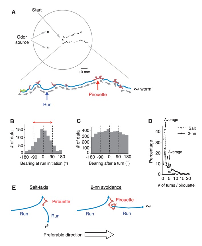
Figure 1.
C.elegans selectively initiates runs away from the odor source.
( A ) Examples of the tracks of 2 animals during 12 min of 2-nonanone avoidance assay, overlaid on a schematic drawing of a 9 cm plate. One of the tracks is magnified below. In the magnified view, pir...
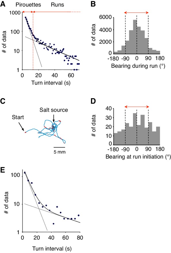
Figure 1u2014figure supplement 1.
Differences between 2-nonanone avoidance behavior and salt-taxis of C.elegans .
( A ) Pirouettes and runs were classified by the length of turn interval ( i.e., migratory durations). A distribution of turn intervals during the odor avoidance was fitted by the sum of two exponenti...
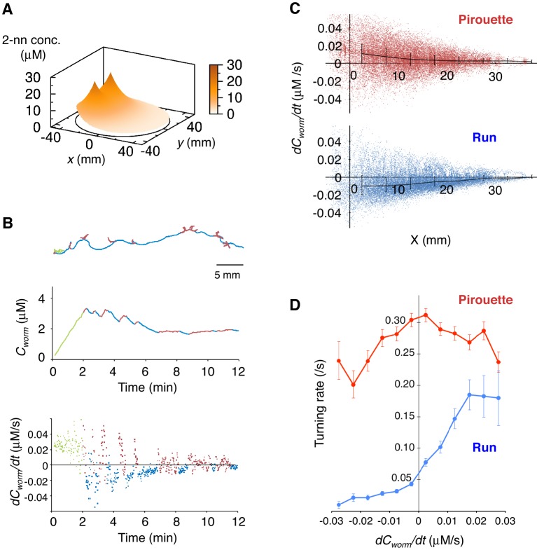
Figure 2.
Pirouettes and runs are distinct behavioral states, which are associated with positive and negative dC worm /dt , respectively.
( A ) Fitted odor gradient over the assay plate at 12 min, based on the actual measurements shown in Figure 2u2014figure supplement 1D . ( B ) (Top) Same with the magnified view of an animal's traject...
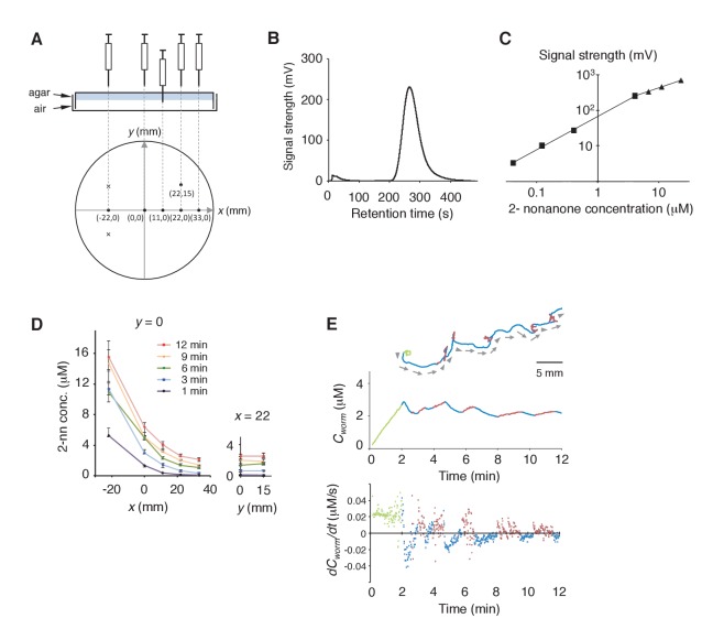
Figure 2u2014figure supplement 1.
Measurement of the gaseous 2-nonanone gradient in the plate assay paradigm.
( A ) A schematic cross-section (upper panel) and top view (lower panel) of gas sampling. The plate is placed upside-down. In the lower panel, crosses indicate positions of the odor source and dots in...
Video 1.
Time-course changes in the fitted 2-nonanone concentration.
Although the odor sources were two circles ofu00a0~5 mm diameter in the real experiment, they were treated as points in the simulation. DOI: http://dx.doi.org/10.7554/eLife.21629.007
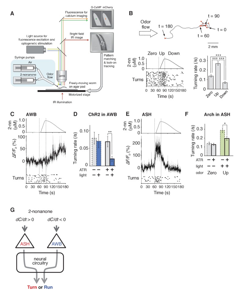
Figure 3.
AWB and ASH sensory neuron pairs regulate turning rate in response to dC/dt of 2-nonanone.
( A ) Schematic drawing of the OSB2 system. ( B ) Behavioral response to temporal changes in the 2-nonanone concentration. (Top) Track of a wild-type animal. The first 60 s (gray) is a period of no od...
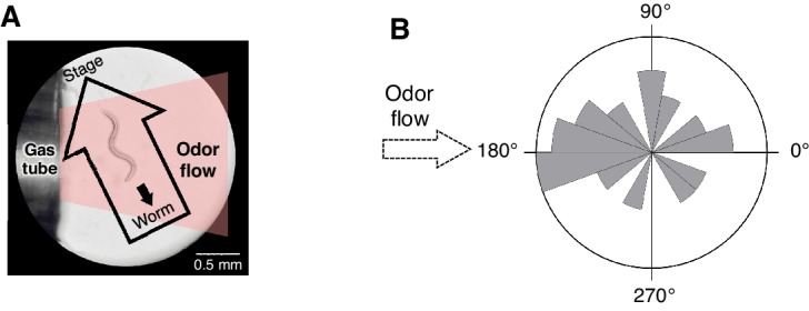
Figure 3u2014figure supplement 1.
Spatial arrangement of the odor stimulation and behavioral response in the OSB2 system.
( A ) Arrangement of the odor flow on the OSB2 system. The end of the tube was positionedu00a0~1 mm from the animal, and odor flow covered the entire body of the animal. Visualization was obtained fro...
Video 2.
A demonstration video for calcium imaging with the OSB2 system.
(Left) The bright field images for the tracking and the fluorescence images for calcium imaging were acquired simultaneously but separately in the tracking and calcium imaging subsystems, respectively...
Video 3.
Visualization of the odor flow on the OSB2 system.
The view was from the ocular lens of the microscope. The tube end was on the left and the flow was from the left to the right, which was visualized by fog produced by Wizard Stick (Zero Toys, USA). Co...
Video 4.
Optogenetic activation of AWB neurons.
After 60 s without any stimulus, a transgenic animal expressing the bistable variant of channelrhodopsin, ChR2(C128S), was illuminated with blue light for 3 s to cause sustained AWB activation, and th...
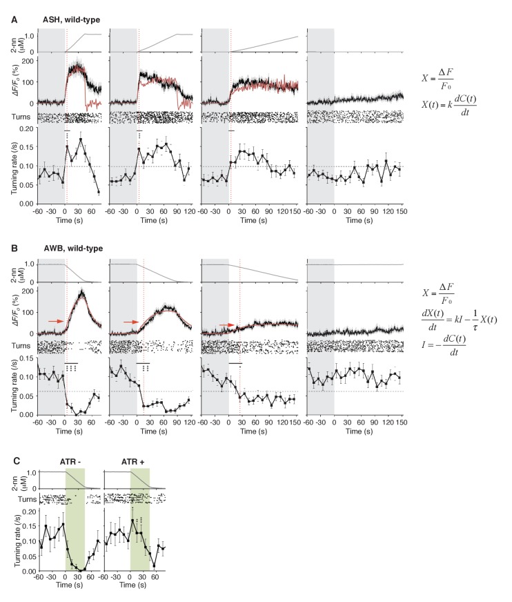
Figure 4.
ASH neurons are activated according to dC/dt for initiating turns, and AWB neurons are activated according to the leaky integration of the negative dC/dt for suppressing turns with a dC/dt -dependent delay.
( A ) ASH responses (middle panels) and turns (lower panels) in response to odor concentration increases from 0 to 1 u03bcM in 45 s (left most; nu00a0=u00a032), 90 s (middle left; nu00a0=u00a039), 180...
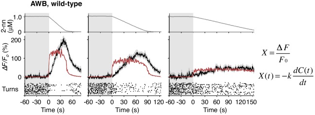
Figure 4u2014figure supplement 1.
AWB responses were not fitted sufficiently by time-differential equations.
The AWB responses are the same as those in Figure 4B . k are described in Table 3 . DOI: http://dx.doi.org/10.7554/eLife.21629.014
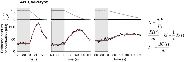
Figure 4u2014figure supplement 2.
Estimated intracellular calcium concentrations in AWB neurons calculated from measured u0394F/F 0 in Figure 4B .
Estimated calcium concentration changes (black lines) in response to odor decreases from 1 to 0 u03bcM in 45 s (left), 90 s (center), and 180 s (right) were also well-fitted by a leaky integrator equa...
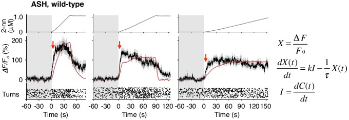
Figure 4u2014figure supplement 3.
ASH responses were partially fitted by the time-integral equations.
The ASH responses are the same as those in Figure 4A . Red arrows indicate the same timing with the red vertical dotted lines in Figure 4A . The parameters and goodness of fit are described in Table 3...
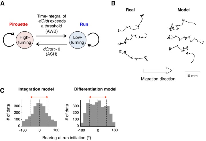
Figure 5.
A computer model reproduced the directional choice in the odor avoidance task in a temporal integration-dependent manner.
( A ) Model of the behavioral transition in 2-nonanone avoidance. During a pirouette, a model animal frequently repeated turns and short migrations. When a model animal initiated a migration away from...
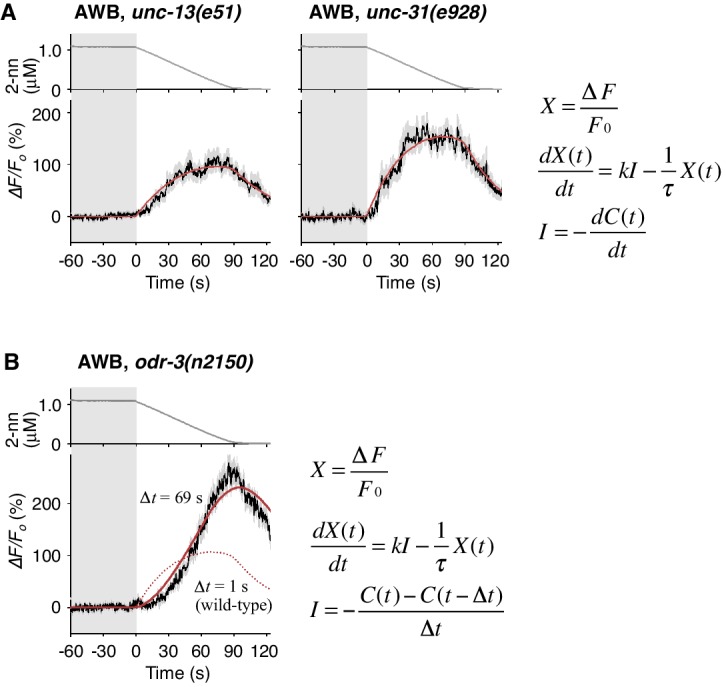
Figure 6.
Cell-autonomous computations in AWB neurons.
( A ) The AWB responses of unc-13 (left) and unc-31 (right) mutants to the odor decreases, which are the same as those shown in the middle left panel of Figure 4B , were essentially similar to those o...
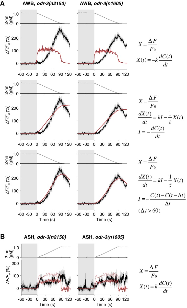
Figure 6u2014figure supplement 1.
Responses of AWB and ASH neurons in odr-3 mutants.
( A ) AWB responses in odr-3(n2150) (left panels; the same data as Figure 6B ) or odr-3(n1605) (right panels; nu00a0=u00a028) mutants were fitted by the right-most equations. When fitting with the lea...
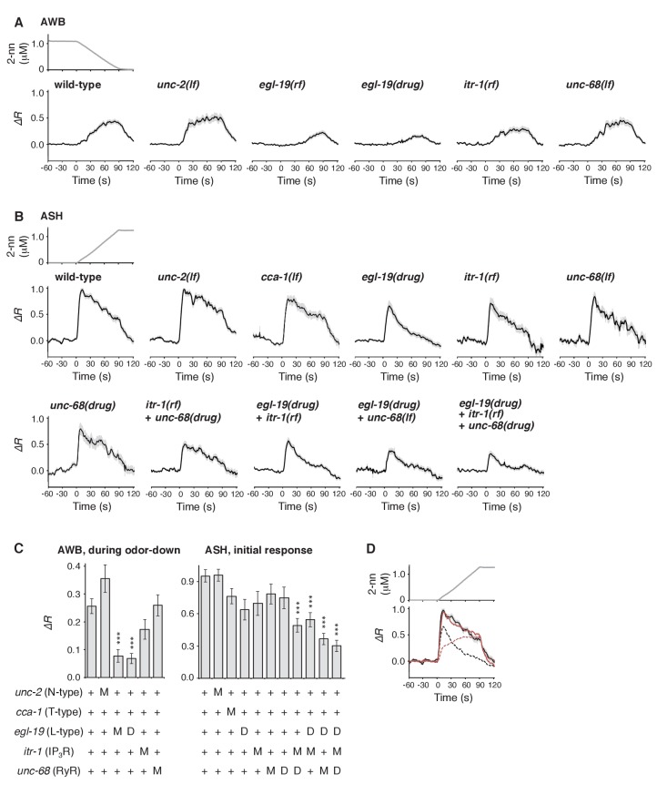
Figure 7.
Calcium channels are involved in the dynamic regulation of [Ca 2+ ] i in a cell type-dependent manner.
( A and B ) Responses of AWB (panel A) or ASH (panel B) neurons in strains with genetic and/or pharmacological suppression of N/P/Q-type VGCC UNC-2, T-type VGCC CCA-1, L-type VGCC EGL-19, IP 3 R ITR-1...
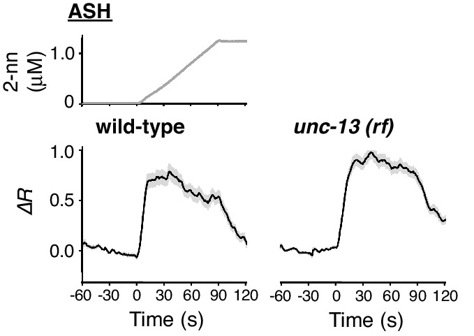
Figure 7u2014figure supplement 1.
ASH response does not depend on synaptic transmission.
ASH responses in wild-type (left; nu00a0=u00a035) and unc-13(e51) (right; nu00a0=u00a044) animals, analysed in parallel, are shown. DOI: http://dx.doi.org/10.7554/eLife.21629.025
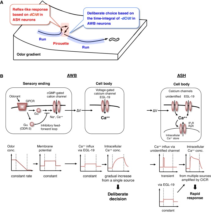
Figure 8.
Physiological and molecular models of decision-making by C. elegans during odor avoidance.
( A ) Computations of ASH and AWB neurons during odor avoidance behavior. ( B ) Model of the molecular mechanisms for temporal computation of odor information in AWB and ASH neurons. (Left) In AWB neu...
Figure images are served from the NIH/NLM PubMed Central Open Access Subset or Europe PMC; copyright remains with the publishers and authors.
💬 Discussion
0 commentsNo comments yet. Be the first to start a discussion!
Leave a Comment