Abstract
Radial spokes (RSs) are ubiquitous components in the 9 + 2 axoneme thought to be mechanochemical transducers involved in local control of dynein-driven microtubule sliding. They are composed of >23 polypeptides, whose interactions and placement must be deciphered to understand RS function. In this paper, we show the detailed three-dimensional (3D) structure of RS in situ in Chlamydomonas reinhardtii flagella and Tetrahymena thermophila cilia that we obtained using cryoelectron tomography (cryo-ET). We clarify similarities and differences between the three spoke species, RS1, RS2, and RS3, in T. thermophila and in C. reinhardtii and show that part of RS3 is conserved in C. reinhardtii, which only has two species of complete RSs. By analyzing C. reinhardtii mutants, we identified the specific location of subsets of RS proteins (RSPs). Our 3D reconstructions show a twofold symmetry, suggesting that fully assembled RSs are produced by dimerization. Based on our cryo-ET data, we propose models of subdomain organization within the RS as well as interactions between RSPs and with other axonemal components.
🔬 Techniques
🔭 Microscopes
🧬 Organisms
💻 Software
🧪 Sample Preparation
🏭 Microscope Brands
💻 Software Details
💾 Data Repositories
🏛️ Research Organizations (ROR)
Affiliated research institutions:
📋 Methods
Cell culture and flagella isolation The C. reinhardtii 137c
WT and pf1 , pf24 , and pf14 mutant strains used in this study ( Table I ) were obtained from the Chlamydomonas Genetics Center. WT and mutant strains were cultured in TAP (Tris-acetate-phosphate) medium ( Gorman and Levine, 1965 ). Data from the C. reinhardtii ida4 mutant were obtained from a previous study ( Bui et al., 2008 ). T. thermophila WT cells obtained from the Tetrahymena Stock Center were used and cultured in proteose peptone medium ( Orias et al., 2000 ). Flagella and cilia from both organisms were isolated using the dibucaine method to induce deflagellation ( Witman, 1986 ). The flagella were sedimented at 5,200 g for 20 min at 4°C, demembranated with 30 mM Hepes, pH 7.4, 5 mM MgSO 4 , 1 mM DTT, 0.5 mM EDTA, 25 mM KCl, and 0.8% NP-40, and sedimented again at 5,200 g for 60 min at 4°C. The pellet of axonemes was resuspended in 30 mM Hepes, pH 7.4, 5 mM MgSO 4 , 1 mM DTT, 0.5 mM EDTA, and 25 mM KCl and stored at 0°C before plunge freezing. Quick plunge freezing and cryo-ET The specimen was frozen with liquid ethane at liquid nitrogen temperature using a vitrification device (Vitrobot; FEI) and grids (Quantifoil Micro Tools GmbH) with holey carbon support film (200 mesh copper grid; R2/2; Quantifoil Micro Tools GmbH). 10-nm gold colloidal particles were applied on the grids during sample preparation and used later as fiducial markers for tomographic reconstruction. The grids with frozen-hydrated samples were transferred to a cryoholder (626; Gatan) cooled by liquid nitrogen. Images were collected as described previously ( Ishikawa et al., 2007 ; Bui et al., 2008 , 2009 ; Movassagh et al., 2010 ) using a transmission electron microscope (Tecnai F20; FEI) equipped with a field emission gun, an energy filter (GIF Tridiem; Gatan), and a 2,048 × 2,048 charge-coupled device camera (UltraScan 1000; Gatan) at the accelerating voltage of 200 kV, a magnification of 19,303×, and an under focus of 3–5 µm. Tomographic image series from −60 to 60°, with 2° tilt increments, were acquired using Explore3D software (FEI). Images were collected with a 0.1–0.2-s exposure time and energy filter width of 20 V. To select round-shaped flagella embedded in ice and to avoid deformation caused by compression (flattening), we carefully chose axonemes having a diameter of 220 nm (measured on single images) and later screened in 3D ( Bui et al., 2009 ).
Show full methods section
Cell culture and flagella isolation The C. reinhardtii 137c
WT and pf1 , pf24 , and pf14 mutant strains used in this study ( Table I ) were obtained from the Chlamydomonas Genetics Center. WT and mutant strains were cultured in TAP (Tris-acetate-phosphate) medium ( Gorman and Levine, 1965 ). Data from the C. reinhardtii ida4 mutant were obtained from a previous study ( Bui et al., 2008 ). T. thermophila WT cells obtained from the Tetrahymena Stock Center were used and cultured in proteose peptone medium ( Orias et al., 2000 ). Flagella and cilia from both organisms were isolated using the dibucaine method to induce deflagellation ( Witman, 1986 ). The flagella were sedimented at 5,200 g for 20 min at 4°C, demembranated with 30 mM Hepes, pH 7.4, 5 mM MgSO 4 , 1 mM DTT, 0.5 mM EDTA, 25 mM KCl, and 0.8% NP-40, and sedimented again at 5,200 g for 60 min at 4°C. The pellet of axonemes was resuspended in 30 mM Hepes, pH 7.4, 5 mM MgSO 4 , 1 mM DTT, 0.5 mM EDTA, and 25 mM KCl and stored at 0°C before plunge freezing. Quick plunge freezing and cryo-ET The specimen was frozen with liquid ethane at liquid nitrogen temperature using a vitrification device (Vitrobot; FEI) and grids (Quantifoil Micro Tools GmbH) with holey carbon support film (200 mesh copper grid; R2/2; Quantifoil Micro Tools GmbH). 10-nm gold colloidal particles were applied on the grids during sample preparation and used later as fiducial markers for tomographic reconstruction. The grids with frozen-hydrated samples were transferred to a cryoholder (626; Gatan) cooled by liquid nitrogen. Images were collected as described previously ( Ishikawa et al., 2007 ; Bui et al., 2008 , 2009 ; Movassagh et al., 2010 ) using a transmission electron microscope (Tecnai F20; FEI) equipped with a field emission gun, an energy filter (GIF Tridiem; Gatan), and a 2,048 × 2,048 charge-coupled device camera (UltraScan 1000; Gatan) at the accelerating voltage of 200 kV, a magnification of 19,303×, and an under focus of 3–5 µm. Tomographic image series from −60 to 60°, with 2° tilt increments, were acquired using Explore3D software (FEI). Images were collected with a 0.1–0.2-s exposure time and energy filter width of 20 V. To select round-shaped flagella embedded in ice and to avoid deformation caused by compression (flattening), we carefully chose axonemes having a diameter of 220 nm (measured on single images) and later screened in 3D ( Bui et al., 2009 ).
Image analysis
Tomograms were reconstructed by IMOD ( Mastronarde, 1997 ) with fiducial marker alignment and R-weighted back projection. Subtomograms with pixel dimensions of 200 × 200 × 200 (∼137 nm in each dimension) were boxed out with a roughly 96-nm period from the original tomogram by Bsoft ( Heymann, 2001 ) and aligned along the microtubule by SPIDER ( Frank et al., 1996 ) followed by intermicrotubule alignment ( Bui et al., 2008 ). Averages were always deconvoluted by the total contribution of the missing wedge to keep data sampling isotropic as described in Bui et al. (2008) . In brief, the deconvolution was performed by dividing the Fourier transformation of the averaged map by the weight from the contributions of missing wedges from all the original subtomograms, which have different orientations. Surface rendering was performed using the University of California, San Francisco Chimera software ( Pettersen et al., 2004 ) after masking, denoising by a band-pass filter, and contrast inversion. The difference maps were generated using University of California, San Francisco Chimera ( Pettersen et al., 2004 ). The resolution of the reconstructions was measured using even/odd Fourier shell correlation between independent copies of the volume using the 0.5 criterion. Mass estimations of the head, neck, and stalk of the RS complex were calculated using the average density of 1.43 g/cm 3 for proteins ( Quillin and Matthews, 2000 ) and after normalizing the isosurface-rendering threshold to the mass of microtubules. The density maps of RS1 and RS2 were deposited in the EM Data Bank (accession no. EMD-1941). Online supplemental material Fig. S1 shows the Fourier shell correlation curve used to evaluate the resolution (in angstroms) of the 3D reconstruction shown in Fig. 1 and Fig. 2 . Fig. S2 shows details of the interactions of the C. reinhardtii RS2 with the A-microtubule and the dynein c tail. Fig. S3 shows the connection of the T. thermophila RS3 with the head of dynein g/b. Video 1 shows the surface rendering of averaged axonemal 96-nm repeats from WT C. reinhardtii (the RSs are colored in yellow). Video 2 shows the surface rendering of the RS domains based on C. reinhardtii mutant analysis. Online supplemental material is available at http://www.jcb.org/cgi/content/full/jcb.201106125/DC1 .
Online supplemental material Fig. S1 shows the Fourier shell correlation curve used to evaluate the resolution (in angstroms) of the 3D reconstruction shown in Fig. 1 and Fig. 2 . Fig. S2 shows details of the interactions of the C. reinhardtii RS2 with the A-microtubule and the dynein c tail. Fig. S3 shows the connection of the T. thermophila RS3 with the head of dynein g/b. Video 1 shows the surface rendering of averaged axonemal 96-nm repeats from WT C. reinhardtii (the RSs are colored in yellow). Video 2 shows the surface rendering of the RS domains based on C. reinhardtii mutant analysis. Online supplemental material is available at http://www.jcb.org/cgi/content/full/jcb.201106125/DC1 .
📊 Figures
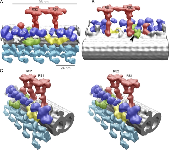
Figure 1.
Overall 3D architecture of the C. reinhardtii axonemal microtubule doublet (96-nm repeat). These surface renderings of 3D structure were averaged from 2,400 subtomograms and include the microtubule do...
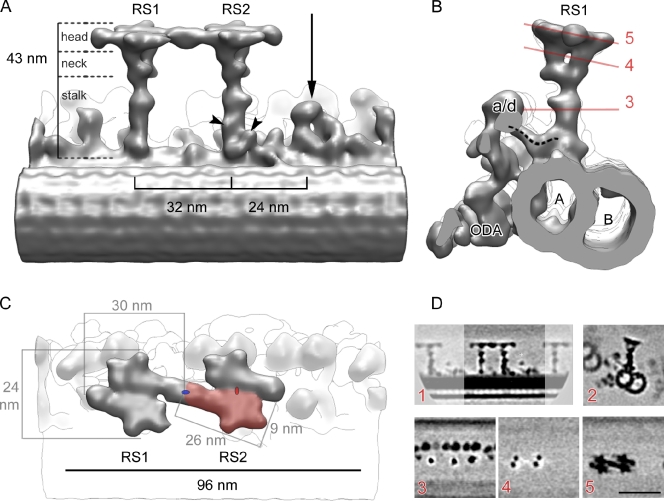
Figure 2.
3D reconstruction of WT RSs in C. reinhardtii. (Au2013C) Surface renderings of tomographic reconstruction after 3D subtomogram averaging. (A) Longitudinal view showing the B-microtubule (foreground), ...
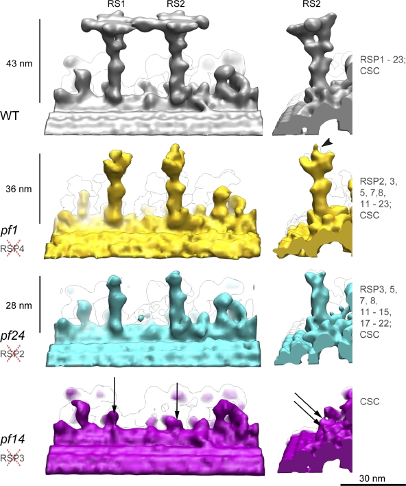
Figure 3.
Comparison of the 3D structure of RSs from three mutants and WT cells. (left) The proximal end is to the left. (right) The same model but oriented so that the distal end of the axoneme points toward t...
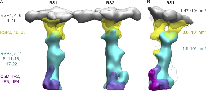
Figure 4.
RS domains. Differential maps show the boundaries between the various domains of the RS structure (gray, heads; yellow, necks; blue, stalks; purple, adaptor protein complexes). (A) Longitudinal view w...
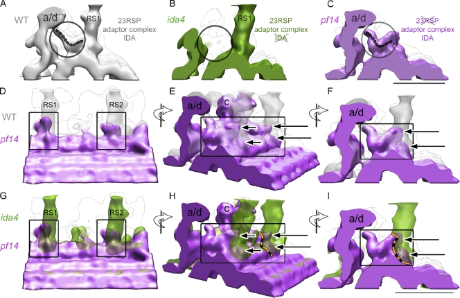
Figure 5.
Localization of adaptor complexes at the RS bases in C. reinhardtii . (A) Portion of the WT reconstruction showing the RS1 stalk, IDA a/d, and dynein a/d tail (encircled). The dashed gray line traces ...
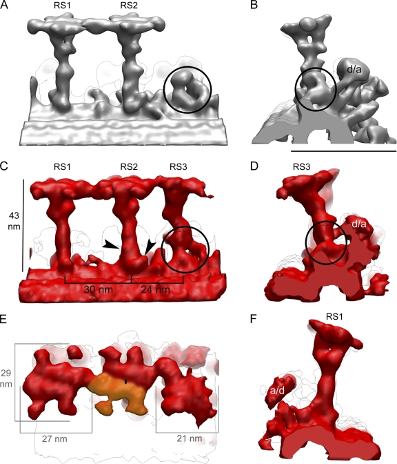
Figure 6.
3D structure of RSs in T. thermophila and RS3 in C. reinhardtii . (A and B) Longitudinal (proximal end of the axoneme to the left; A) and side (as seen from the distal end; B) views of the WT C. reinh...
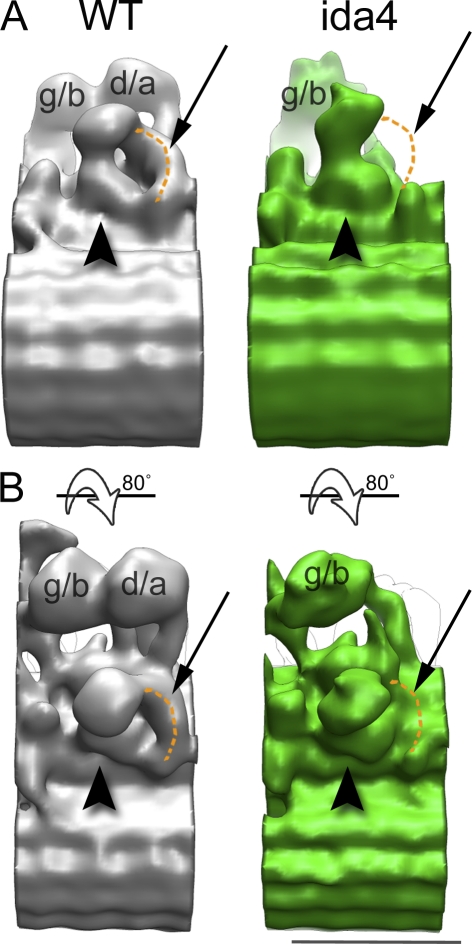
Figure 7.
RS3 and the tail of IDA d/a. 3D reconstruction of RS3 stumps from WT (gray; left) and ida4 (green; right) flagella. (A) View from the adjacent doublet microtubules. The proximal end of the axoneme is ...
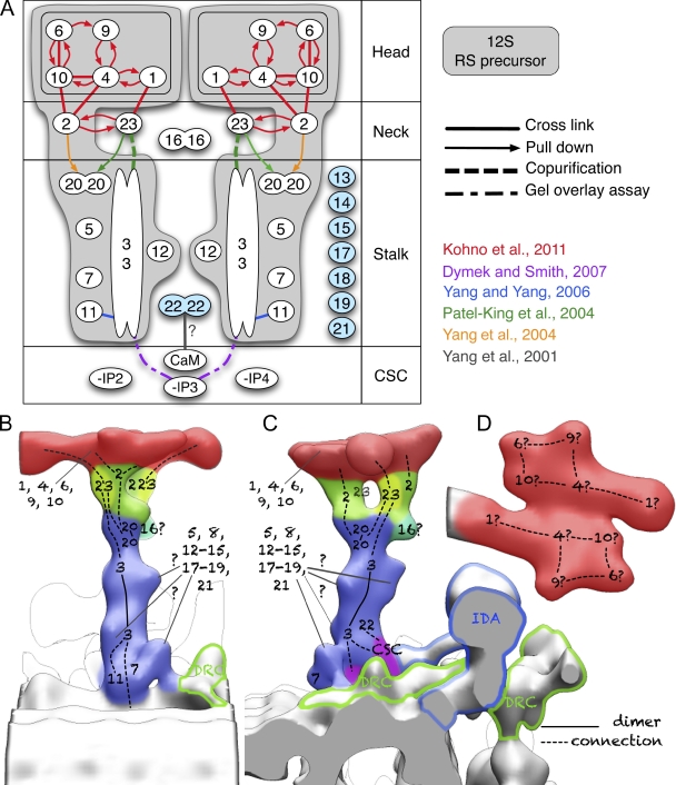
Figure 8.
Model for RS structure. (A) The diagram summarizes current knowledge about the protein composition and the stoichiometry of one ideal RS. Assignment of the 23 RSPs to the four domains (head, neck, sta...
Figure images are served from the NIH/NLM PubMed Central Open Access Subset or Europe PMC; copyright remains with the publishers and authors.
💬 Discussion
0 commentsNo comments yet. Be the first to start a discussion!
Leave a Comment