Abstract
Abstract The promise of single-objective light-sheet microscopy is to combine the convenience of standard single-objective microscopes with the speed, coverage, resolution and gentleness of light-sheet microscopes. We present DaXi, a single-objective light-sheet microscope design based on oblique plane illumination that achieves: (1) a wider field of view and high-resolution imaging via a custom remote focusing objective; (2) fast volumetric imaging over larger volumes without compromising image quality or necessitating tiled acquisition; (3) fuller image coverage for large samples via multi-view imaging and (4) higher throughput multi-well imaging via remote coverslip placement. Our instrument achieves a resolution of 450 nm laterally and 2 μm axially over an imaging volume of 3,000 × 800 × 300 μm. We demonstrate the speed, field of view, resolution and versatility of our instrument by imaging various systems, including Drosophila egg chamber development, zebrafish whole-brain activity and zebrafish embryonic development – up to nine embryos at a time.
🔬 Techniques
🧬 Organisms
💻 Software
✨ Fluorophores
🧪 Sample Preparation
🏭 Microscope Brands
🧪 Reagent Suppliers
📷 Detectors
🎨 Filters
💻 Software Details
💻 Code & Software
Dataset EXploration & Processing
Hierarchical Graph Analysis
python functions for simulating optical transfer functions
💾 Data Repositories
🏛️ Research Organizations (ROR)
Affiliated research institutions:
📋 Methods
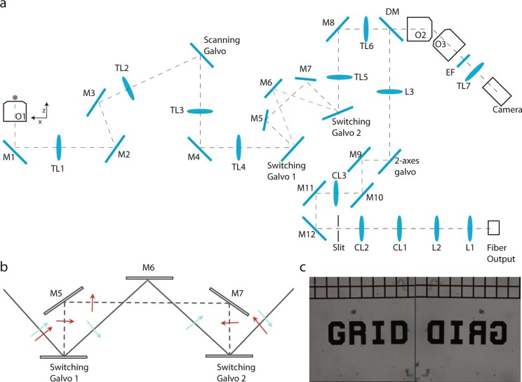
Microscope description Extended Data Fig. 1 shows the detailed optical setup. A primary objective (O 1 , Olympus XLUMPLFLN 20XW NA1.0, water) is used to both generate an oblique light sheet in the sample and to collect the fluorescence. A series of tube lenses (TL1 to TL6) conjugate the pupils of O 1 and O 2 so that an intermediate image of the sample at O 1 is formed at the secondary objective O 2 (Olympus UPLXAPO20X). The intermediate image has a uniform magnification of 1:33, equal to the refractive index ratio of the medium of O 1 versus that of O 2 , making the optical train aberration-free over a reasonable volume 20 , 35 . A custom tertiary objective O 3 (AMS-AGY v.2.0, Supplementary Figs. 5 – 7 and Supplementary Note 3 ) is oriented by 45° with respect to O 2 . The fluorescence is filtered by either individual bandpass filters (Chroma ET525/50, ET605/70) or a quad-band filter (Chroma ZET405/488/561/640) and then detected by a scientific complementary metal-oxide semiconductor (sCMOS) camera (Hamamatsu ORCAFlash 4.0). The pixel size of the cameras at the sample space is 146 nm (TL7—Thorlabs AC300A) for PSF calibration and 265 nm (TL7—Thorlabs TTL165-A) or 440 nm (TL7—Thorlabs TTL100-A) for imaging so as to capture the desired field of view. Objective O 3 is mounted on a piezo stage (PI Fast PIFOC Z-Drive PD72Z1SAQ) so that its focus can be finely adjusted. Two switching galvo mirrors are used to create two views of the object in the sample space. By adjusting the angles of the two galvo mirrors, the light is reflected either by just one or by two reflective mirrors. The operating principle is similar to that of a Dove prism. Moreover, the switching module also changes the incident angle of the light sheet between +45° and −45° since the excitation light also passes through this module. Illumination and detection scanning. A galvo mirror (Cambridge Tech, 20 mm galvo, 6SD12205) is conjugated to the pupil planes of both O 1 and O 2 . Rotating the galvometer actuated mirror scans the oblique light sheet across the sample (along the x axis), with the incident angle kept at 45°. The galvo mirror also descans the intermediate image at the focal space of O 2 so that the intermediate image is always projected at the focal plane of O 3 . Using the galvometer for 3D scanning allows for faster imaging compared to stage scanning, but at the cost of a limited scan range of approximately 300 µm. A motorized stage (ASI MS-2000) is used to position the sample and to perform scanning for volumetric imaging. During acquisition of each frame, stage scanning is combined with galvo descanning to stabilize the imaging plane (coplanar light sheet and detection planes) relative to the sample. In the absence of relative motion between the sample and the imaging plane, no motion blur occurs. Stabilized light-sheet stage scanning allows for much longer ranges compared to galvometer-based scanning. It is only limited by the range of travel of the stage, in our case 75 mm. Illumination and detection planes remain fixed and optimally placed at the center of O 1 and O 2 native axes thus guaranteeing optimal light collection, minimal aberrations and thus optimal image quality. For long-term imaging, a water dispenser was built to automatically supply immersion water between the primary objective and the sample (Supplementary Fig. 3 ). The water dispenser consists of a micropump (part of a Leica Water Immersion Micro Dispenser), a microcapillary tip (Eppendorf Microloader) and a 3D-printed objective cap. An environmental chamber (Supplementary Fig. 4 ) was built around the sample to keep it at roughly 28 °C. Supplementary Notes 1 and 2 provide a more detailed description and alignment procedure, Supplementary Fig. 1 contains photos of the actual setup, Supplementary Fig. 2 has an image of the computer-aided design model of the microscope, Supplementary Video 8 shows an animation of the setup and Supplementary Table 5 contains a the list of components used to construct the microscope.
Show full methods section
Microscope description Extended Data Fig. 1 shows the detailed optical setup. A primary objective (O 1 , Olympus XLUMPLFLN 20XW NA1.0, water) is used to both generate an oblique light sheet in the sample and to collect the fluorescence. A series of tube lenses (TL1 to TL6) conjugate the pupils of O 1 and O 2 so that an intermediate image of the sample at O 1 is formed at the secondary objective O 2 (Olympus UPLXAPO20X). The intermediate image has a uniform magnification of 1:33, equal to the refractive index ratio of the medium of O 1 versus that of O 2 , making the optical train aberration-free over a reasonable volume 20 , 35 . A custom tertiary objective O 3 (AMS-AGY v.2.0, Supplementary Figs. 5 – 7 and Supplementary Note 3 ) is oriented by 45° with respect to O 2 . The fluorescence is filtered by either individual bandpass filters (Chroma ET525/50, ET605/70) or a quad-band filter (Chroma ZET405/488/561/640) and then detected by a scientific complementary metal-oxide semiconductor (sCMOS) camera (Hamamatsu ORCAFlash 4.0). The pixel size of the cameras at the sample space is 146 nm (TL7—Thorlabs AC300A) for PSF calibration and 265 nm (TL7—Thorlabs TTL165-A) or 440 nm (TL7—Thorlabs TTL100-A) for imaging so as to capture the desired field of view. Objective O 3 is mounted on a piezo stage (PI Fast PIFOC Z-Drive PD72Z1SAQ) so that its focus can be finely adjusted. Two switching galvo mirrors are used to create two views of the object in the sample space. By adjusting the angles of the two galvo mirrors, the light is reflected either by just one or by two reflective mirrors. The operating principle is similar to that of a Dove prism. Moreover, the switching module also changes the incident angle of the light sheet between +45° and −45° since the excitation light also passes through this module. Illumination and detection scanning. A galvo mirror (Cambridge Tech, 20 mm galvo, 6SD12205) is conjugated to the pupil planes of both O 1 and O 2 . Rotating the galvometer actuated mirror scans the oblique light sheet across the sample (along the x axis), with the incident angle kept at 45°. The galvo mirror also descans the intermediate image at the focal space of O 2 so that the intermediate image is always projected at the focal plane of O 3 . Using the galvometer for 3D scanning allows for faster imaging compared to stage scanning, but at the cost of a limited scan range of approximately 300 µm. A motorized stage (ASI MS-2000) is used to position the sample and to perform scanning for volumetric imaging. During acquisition of each frame, stage scanning is combined with galvo descanning to stabilize the imaging plane (coplanar light sheet and detection planes) relative to the sample. In the absence of relative motion between the sample and the imaging plane, no motion blur occurs. Stabilized light-sheet stage scanning allows for much longer ranges compared to galvometer-based scanning. It is only limited by the range of travel of the stage, in our case 75 mm. Illumination and detection planes remain fixed and optimally placed at the center of O 1 and O 2 native axes thus guaranteeing optimal light collection, minimal aberrations and thus optimal image quality. For long-term imaging, a water dispenser was built to automatically supply immersion water between the primary objective and the sample (Supplementary Fig. 3 ). The water dispenser consists of a micropump (part of a Leica Water Immersion Micro Dispenser), a microcapillary tip (Eppendorf Microloader) and a 3D-printed objective cap. An environmental chamber (Supplementary Fig. 4 ) was built around the sample to keep it at roughly 28 °C. Supplementary Notes 1 and 2 provide a more detailed description and alignment procedure, Supplementary Fig. 1 contains photos of the actual setup, Supplementary Fig. 2 has an image of the computer-aided design model of the microscope, Supplementary Video 8 shows an animation of the setup and Supplementary Table 5 contains a the list of components used to construct the microscope.
Optical setup characterization
The microscope’s PSF was measured using 100-nm green fluorescence beads. The beads are first embedded in agarose gel (0.5%) and then deposited on a glass coverslip (no. 1.5). The resulting images are then deskewed to the objective-aligned frame of reference ( xyz coordinates). The positions of the beads are then detected using by finding the local maxima and a cropped image of each bead is used for further analysis. To account for the tilted PSF with respect to the z axis, the cropped images are rotated in the xz plane so that the long axis of the PSF ( z ” axis) is along the z axis. The PSFs are then fitted with a one-dimensional Gaussian function along all three axes ( x ”, y and z ”). The values of the FWHM are then averaged from all fluorescence beads in the imaging volume.
Light-sheet incident angle adjustment and stripe reduction
A two-axis galvo mirrors (Cambridge 10 mm 6SD12056) are conjugated with the sample plane so that rotating the two mirrors results in a rotation of the excitation beam at the sample plane. In particular, the incident angle of the light sheet at the focal space of O 1 can be adjusted by one of the mirrors to 45° with respect to the optical axis. The effective excitation NA is estimated to be 0.08 at this incident angle. The effective excitation NA can be potentially increased, either through reducing the incident angle of the light sheet or using objectives with higher NA. Increasing excitation NA would allow generating a thinner light sheet to further improve the axial resolution but at the expense of field of view 36 – 38 . To reduce the stripe due to sample absorption and obstruction of the illumination light, the light sheet is swept continuously from −6° to 6° (Supplementary Fig. 14 ) in the illumination plane during the acquisition of each frame, using the other mirror of the two-axis galvo.
Microscope control software
The data acquisition and display is done by the open-source, freely available software Micro-Manager 2.0 Gamma 39 . A custom-developed micromanager script sets up the acquisition order and stores the hyperstack data in TIFF files. A NI DAQ system programmed using a Python module controls the timing of all devices during acquisition. The NI DAQ system consists of one compact chassis (cDAQ-9178), two analog control modules (NI 9263 4-Channel AO) and one digital control module (NI 9401 8-channel DIO). The Python module uses the NI-DAQmx Python API to program the DAQ system. It synchronizes the devices, including camera, motorized stage, galvo mirrors and lasers during data acquisition. Alternatively, one can also use Pycromanager 40 to perform data acquisition in the Python environment instead of the Java environment of Micro-Manager. The water dispenser is controlled by another Python module to supply water to the primary objective during long-term recordings. Image processing library: dataset exploration and processing All data processing is done using our open-source Python package dataset exploration and processing (dexp). This library performs a number of image processing tasks specific to light-sheet imaging including equalization, denoising, dehazing, registration, fusion, stabilization, deskewing and deconvolution. It leverages napari 41 for multi-dimensional visualization and 3D rendering, CuPy 42 for graphical processing unit- (GPU-) accelerated computing, Dask 43 for scalable array computing and zarr 44 as multi-dimensional data storage format.
Image processing pipeline
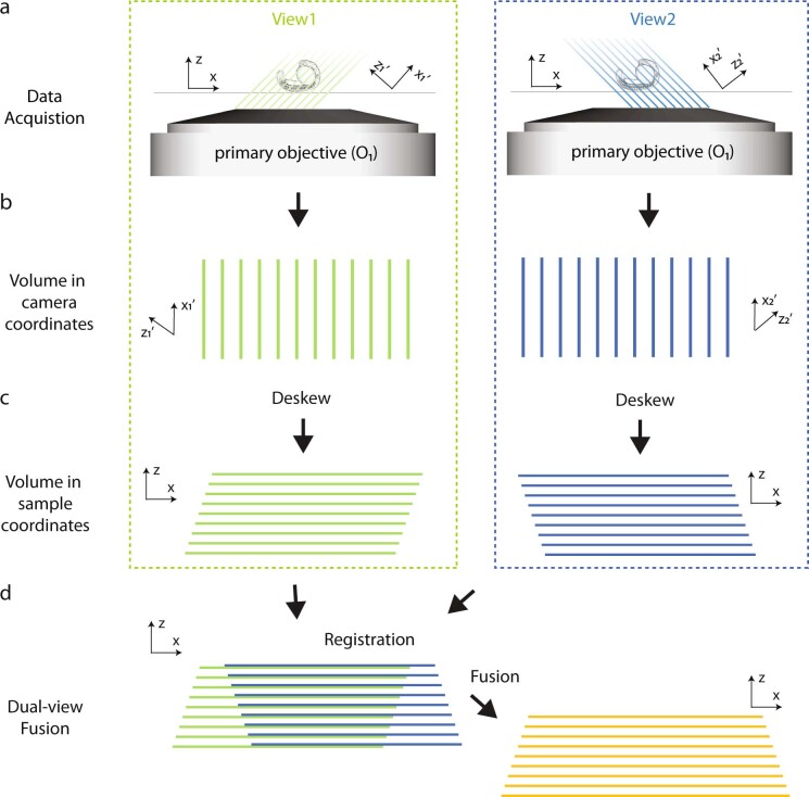
The multi-dimensional data are saved by Micro-Manager to local storage of the control PC in TIFF format. The TIFF files are then read out and converted to zarr format where typically a five- to tenfold data compression is achieved through lossless compression. The zarr datasets are then transferred to a local server equipped with 200 TB storage and 4 NVIDIA Tesla V100 SXM2 32 GB for further processing. The data processing pipeline is shown in Extended Data Fig. 10 . Each 3D stack from one of the views is deskewed to coverslip-based coordinates, that is the xyz coordinates (Supplementary Fig. 15 ). The images are then dehazed to remove large-scale background light caused by scattered illumination and out-of-focus light. The image from the second view is then registered to the first view using an iterative multi-scale warping approach (Supplementary Fig. 16 ). In each iteration, the images are divided into chunks along all three axes by a factor of 2 i where i is the current iteration number; corresponding chunks from both views are registered separately with a translation model to produce a translation vector; a vector field is then calculated based on all the translation vectors and the image of the second view is warped according to the vector field. This procedure repeats until the maximum number of iterations or the minimal size of the chunk is reached. In this work, the maximum iteration number was set to four and the minimal chunk size 32 × 32 × 32. This procedure results in a spline-interpolated vector field that is applied to the second view. After registration, images from the two views are fused by picking regions from one or the other image based on the local image quality 45 . The magnitude of the Sobel gradient was used as the metric to generate a blend map, based on which the two images are blended. Other fusion methods such as frequency domain fusion (discrete cosine transform, fast Fourier transform) are available in dexp. An illumination intensity correction is applied to the fused data to account for the Gaussian profile of the light sheet along the y axis. Each raw data per time point is around 8 GB (two views, roughly 1,000 × 1,024 × 2,048 × 2 voxels). An 8-hour continuous imaging session produces roughly 8 TB of raw data (roughly 1,000 time points). It takes roughly 1 min to process the data per time point per GPU and 4 h to process the whole dataset with four GPUs running in parallel. After all time points are processed, they are temporally stabilized to compensate minor drifts over time. Temporal stabilization Temporal stabilization is performed by computing for each time point, the relative displacement vector to its 2 × n neighbors, where n is typically chosen to be 7. The displacement vector between two 3D images is simply computed by phase correlation. Once all these relative shifts are obtained, we formulate and solve the linear system: R = M A in which A is the vector of ‘absolute’ positions of the sample, M is the band matrix that encodes the relationship between absolute and relative shifts and R is the vector of observed relative shifts. The goal is to recover the absolute positions A from the relative measurements R . A simple approach is to simply invert this linear system in a least-square sense. However, in practice the measurements that constitute R can be affected by noise, and so we use L 1 regularized inversion to obtain the best results. The code can be found at https://github.com/royerlab/dexp/blob/master/dexp/processing/registration/sequence.py.
Video rendering
Color max-projection rendering is done using code implemented as part of our dexp library ( https://github.com/royerlab/dexp ). Some of the more complex volume rendering videos involving rotations are done with napari-animation 41 ( https://github.com/royerlab/dexp ): an easy to use napari plugin ( https://napari.org/ ) capable of complex keyed animation.
Segmentation and tracking
The nuclei segmentation and tracking are computed jointly using the approach presented by Türetken et al. 46 . First, the 3D cell boundaries are predicted using a neural network 47 . The predicted cell boundaries are then fed to a hierarchical watershed algorithm from Higra 48 (github.com/higra/Higra), to generate an initial set of segments by accounting for partial occlusions and overlaps. Last, the tracking algorithm then picks the optimal segments that maximize the total integer programming cost 46 . We define the individual integer programming cost to connect the segments between adjacent time points as the intersection over union of their masks. The flow fields of the nine fish tails were produced by smoothing the tracklets with Savitzky–Golay filtering and coloring them with their track identifiers, which is correlated with the time point of their appearance. The tracks of the whole embryo were colored with the orientation of the flow field 49 .
Sample preparation
Zebrafish husbandry and experiments were conducted according to protocols approved by the UCSF Institutional Animal Care Use Committee. In the experiments, we used tg(h2afva:h2afva-mCherry (a gift from J. Huisken, Morgridge Institute for Research) and for the functional imaging of neuronal activity, we used tg(elevl3:GCaM6f) and tg(elavl3:H2B-GCaMP6s) 50 . The sample mounting geometry is shown in Supplementary Figs. 17 and 18 . First, zebrafish were dechorionated with a pair of sharp forceps underneath a binocular dissecting microscope and incubated for at least 5 min in a solution of fish water and tricaine (0:016%). Embryos were gently pipetted into a 0:1% solution of low gelling point agarose (Sigma, A0701) cooled at 37 °C. The embryos, together with approximately 1 ml of 0:1% agarose, were placed in a glass-bottomed petri dish (Stellar Scientific catalog no. 801001). Using a capillary needle, the embryo was gently positioned at the center of the dish and in the desired orientation: laterally in this case. When the agarose was solidified, the dish was flooded with fish water and 0:016% tricaine. All time-lapse experiments were done with a gentle flow of embryo medium water with 0.016% tricaine at 28 °C, using peristaltic pumps, allowing normal development of the embryo and meanwhile preventing embryo movement. However, occasionally it was possible to observe sudden embryo movements during recordings that resulted in image artifacts: for example, one in Supplementary Video 3 (at roughly 4 min of video time and roughly 63 min of experiment time) and multiple occasions in Supplementary Video 4 . For the calcium imaging experiment fish were embedded in 2% agarose (Sigma, A0701) and anesthetized in an external solution with tricaine (0.2 mg ml −1 ) at 5 dpf. For Drosophila fly imaging, the egg chambers were dissected and cultured as described previously 51 . D. melanogaster ovaries were removed from females 3 d after eclosion for observation. Fly stocks Usp10-Gal4 (BDSC-76169) and UAS-GFP.nls (BDSC-4776) were used. The egg chambers were then transferred to a glass-bottomed petri dish for imaging. The mounting was similar to that used for the zebrafish imaging, except that the egg chambers were immersed in imaging media (Schneider’s media supplied with 200 μg ml −1 insulin, 15% (vol/vol) FBS, 0.6× penicillin–streptomycin, pH 6.95–7.0.) rather than agarose solution.
Imaging conditions
Imaging conditions for all experiments can be found at Supplementary Table 6 .
Statistics and reproducibility
Each experiment was repeated three times for Fig. 3a , 17 times for Fig. 3c,d , eight times for Fig. 4a–f and Supplementary Fig. 12 , three times for Fig. 5b,c , five times for Extended Data Fig. 7 , three times for Extended Data Fig. 8 , three times for Extended Data Fig. 9 and seven times for Supplementary Fig. 13 . Reporting Summary Further information on research design is available in the Nature Research Reporting Summary linked to this article.
Online content Any methods, additional references, Nature Research reporting summaries, source data, extended data, supplementary information, acknowledgements, peer review information; details of author contributions and competing interests; and statements of data and code availability are available at 10.1038/s41592-022-01417-2.
Supplementary information Supplementary Information Supplementary Figs. 1–25, Notes 1–3 and Tables 1–6. Reporting Summary Supplementary Video 1 Rotating rendering of a D. rerio (zebrafish) embryo at 30 hpf imaged on DaXi. Illumination wavelength 488 nm. 3,000 × 800 × 300 µm × 1 view. Voxel size 0.440 × 0.440 × 1.806 µm. Single stack acquisition lasted 52 s. Supplementary Video 2 DaXi imaging of egg D. melanogaster (fly) egg chambers 3 d after eclosion. Transgenic line UAS-GFP.nls (BDSC-4776). Illumination wavelength 488 nm. 3,000 × 800 × 300 µm × 1 view. Voxel size 0.440 × 0.440 × 1.806 µm. Acquisition lasted for 2.5 h with an acquisition interval of 27 s for a total 342 time points. Supplementary Video 3 DaXi imaging of a D. rerio (zebrafish) embryo starting at roughly 10 hpf and ending at 18 hpf. Transgenic line h2afva.mCherry. Illumination wavelength 561 nm. 2,200 × 800 × 300 µm × 2 views. Voxel sizes 0.440 × 0.440 × 1.806 µm. Acquisition lasted 9 h with a 30-s acquisition interval for a total of 1,079 time points. Supplementary Video 4 DaXi imaging of a D. rerio (zebrafish) embryo starting at roughly 24 hpf and ending at 32 hpf. Transgenic line h2afva.mCherry. Illumination wavelength 561 nm. 3,000 × 800 × 300 µm × 2 views. Voxel sizes 0.440 × 0.440 × 1.806 µm. Acquisition lasted 8 h with 73-s acquisition interval for a total of 390 time points. Supplementary Video 5 DaXi imaging, nuclei segmentation and cell tracking of a D. rerio (zebrafish) embryo starting at roughly 12 hpf and ending at roughly 18 hpf. Transgenic line h2afva.mCherry. Illumination wavelength 561 nm, 2,200 × 800 × 300 µm × 2 views. Voxel sizes 0.440 × 0.440 × 1.806 µm. Acquisition lasted 6.6 h with 30-s acquisition interval for a total of 791 time points. Supplementary Video 6 High-throughput DaXi imaging of nine D. rerio (Zebrafish) embryos starting at roughly 10 hpf and ending at roughly 16 hpf. Transgenic line h2afva.mCherry. Illumination wavelength 561 nm. 1,000 × 800 × 300 µm × 2 views. Voxel sizes 0.440 × 0.440 × 1.806 µm. Acquisition lasted 4.6 h with 167.5 s per fish per stack for a total of 100 time points. Supplementary Video 7 High-throughput DaXi imaging, nuclei segmentation and cell tracking of nine D. rerio (Zebrafish) embryos starting at roughly 10 hpf and ending at roughly 16 hpf. Transgenic line h2afva.mCherry. Illumination wavelength 561 nm. 1,000 × 800 × 300 µm × 2 views. Voxel sizes 0.440 × 0.440 × 1.806 µm. Acquisition lasted 4.6 h with 167.5 s per fish per stack for a total of 100 time points. Supplementary Video 8 Video abstract illustrating the main concepts behind DaXi: (1) the sample mounting advantages of single-objective light-sheet microscopy for high-throughput imaging, (2) an explanation of stabilized light-sheet scanning (LS3), (3) multi-view imaging for improved coverage, (4) uncompromised resolution with the AMS-AGY v.2.0 ‘Snouty’ custom objective, (5) high-fidelity 3D rendering of the whole microscope and optics setup and (6) the innovations (animation and rendering by L.W. Whitehead).
Supplementary information The online version contains supplementary material available at 10.1038/s41592-022-01417-2.
📊 Figures
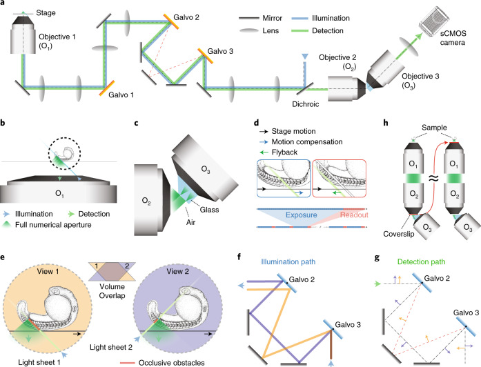
Fig. 1
Design of a high-resolution, large field of view and multi-view single-objective light-sheet microscope.
a , Simplified scheme of the optical setup. b , In this setup, the light-sheet excitation and emission pass through a single objective. The fluorescence is collected by O 1 and relayed downstream with...
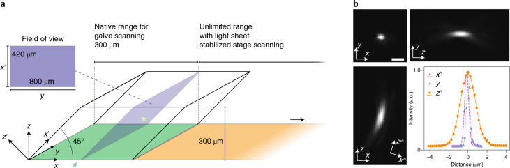
Fig. 2
Characterization of the microscope.
a , Imaging volume geometry. The coverslip is parallel to the xy plane. The optical axis of the microscope is along the z axis (depth). The sample is illuminated by an oblique light sheet in the x u20...
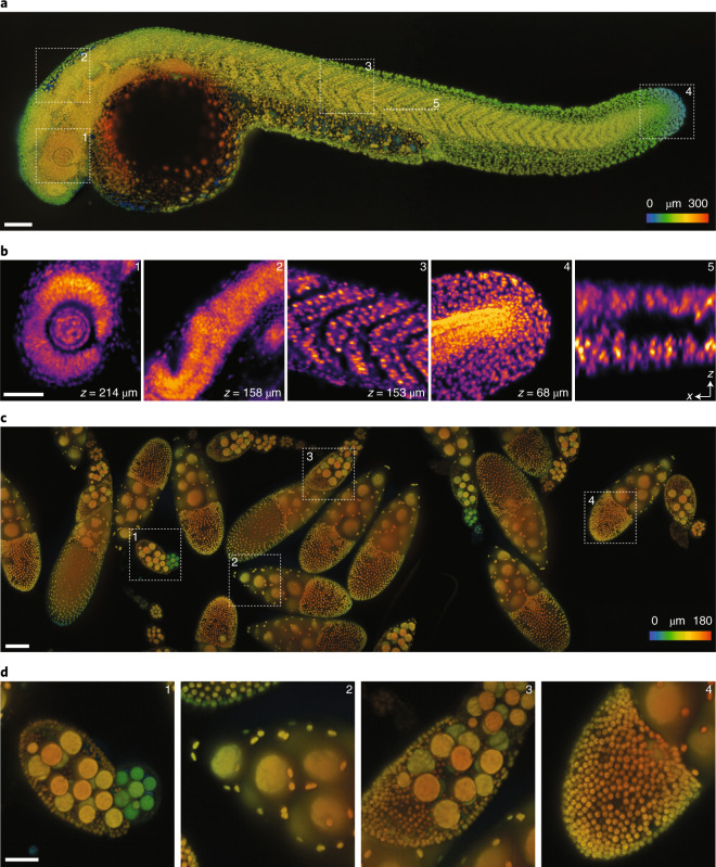
Fig. 3
Large volume imaging of Danio rerio larval development and Drosophila melanogaster egg chambers.
a , Images of a zebrafish larvae (roughly 30u2009hpf, nuclei labeled with tg(h2afva:h2afva-mCherry) imaged using the microscope. Imaging volume ( x , y , z ) is 3,000u2009u00d7u2009800u2009u00d7u20093...
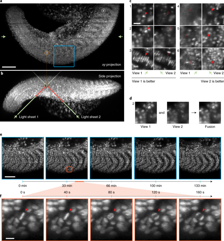
Fig. 4
High-speed multi-view imaging of zebrafish tail development.
a , Axial maximum projection showing the whole zebrafish larva tail at 24u2009hpf, nuclei labeled with tg(h2afva:h2afva-mCherry). Imaging volume is 1,064u2009u00d7u2009532u2009u00d7u2009287u2009u03bcm...
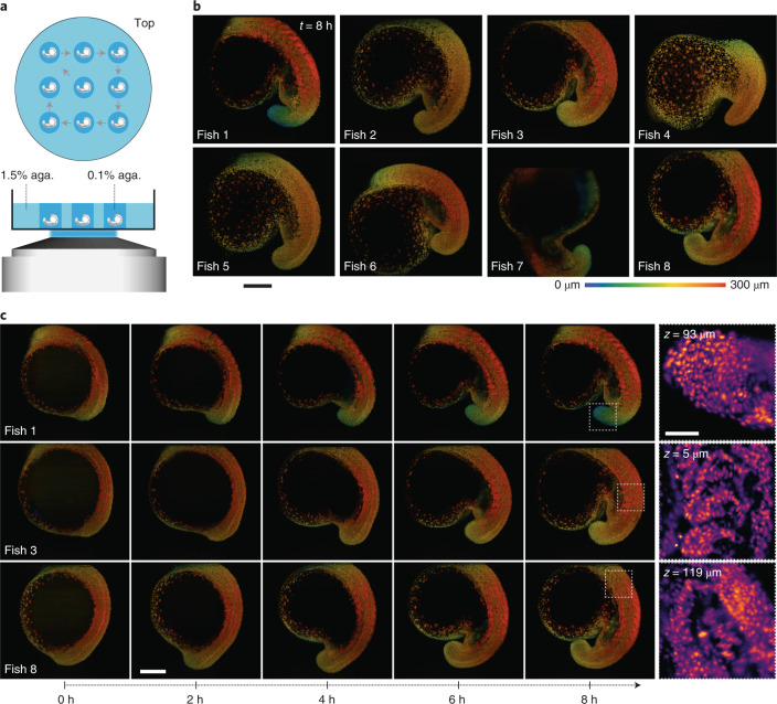
Fig. 5
Imaging nine zebrafish embryos at a time.
a , Top and side views of nine zebrafish embryos mounted in 0.1% agarose gel. b , The embryos (only eight are shown) were imaged sequentially (at 4.5u2009min per round) for up to 8u2009h. Only the fin...
Extended Data Fig. 1
Optical setup of the microscope.
( a ) Detailed layout of the setup. Objectives lenses: O 1 - Olympus XLUMPLFLN 20XW, O 2 - Olympus UPLXAPO20X, O 3 - Calico AMS-AGY v2.0. Tube lenses: TL1, TL2 and TL3 - Olympus SWTLU-C 180u2009mm, TL...
Extended Data Fig. 2
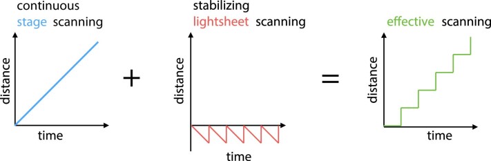
Light sheet stabilized stage scanning (LS 3 ).
During the acquisition of a 3D image stack, the stage moves continuously, and the galvanometer scanner performs a counteracting motion of the light-sheet and detection planes to cancel out any relativ...
Extended Data Fig. 3
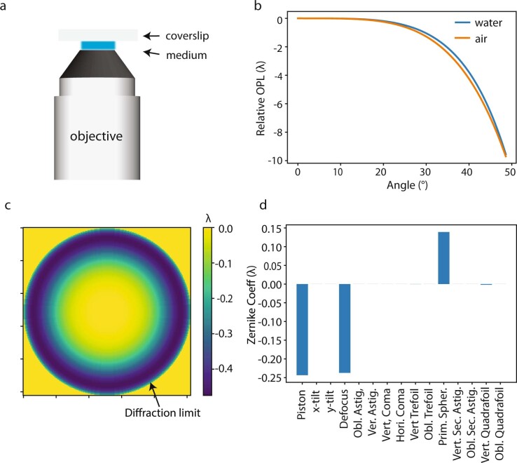
Analysis of the optical path length when placing a glass coverslip into the imaging medium of an objective.
( a ) illustrates the optical system to analyze. Depending on the type of objective, the medium could be air, water, immersion oil, etc. ( b ) plots the optical path length of an emitter at the covers...
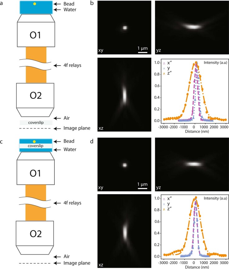
Extended Data Fig. 4
Converting the microscope from upright to inverted by repositioning the coverslip in a remote focusing system.
( a ) shows the remote focusing system composed of two objectives whose pupil planes are conjugated by a 4u2009f relay system. Yellow dot: fluorescent bead. O 1 : 20x, 1.0NA, water dipping. O 2 : 20x,...
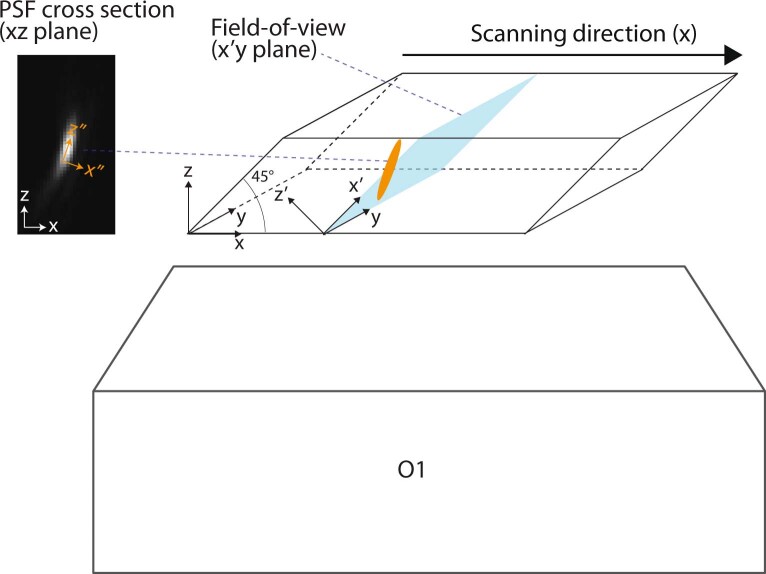
Extended Data Fig. 5
Coordinate system of the microscope.
The objective front lens is parallel to the xy plane. The optical axis of the microscope is along the z axis (depth). The sample is illuminated by an oblique light sheet in the xu2019y plane, where xu...
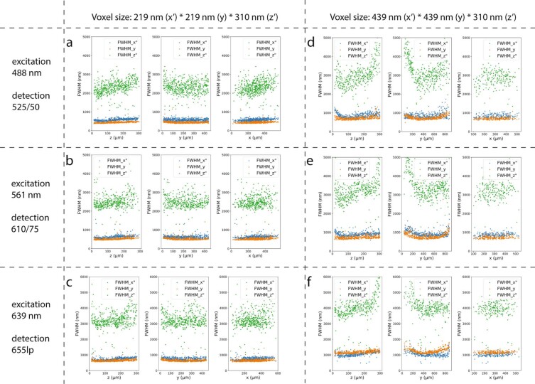
Extended Data Fig. 6
PSF measurements across the imaging volume.
In order to have a good sampling of the PSF for accurate estimation of the resolution, we set the effective magnification to 29.6 and the pixel size to 220u2009nm. With the chip size of our camera bei...
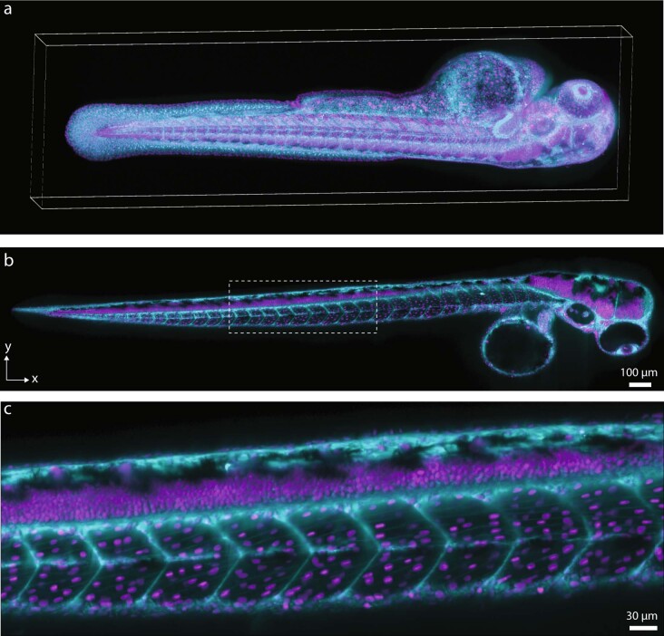
Extended Data Fig. 7
Dual color imaging of a zebrafish larvae.
The larvae is imaged at 2 dpf. The nuclei (magenta) are labelled with tg(h2afva:h2afva-mCherry). The membranes (cyan) are stained using Vybrant DiO cell-labeling solution (Thermal fisher V22889 ). Dio...
Extended Data Fig. 8
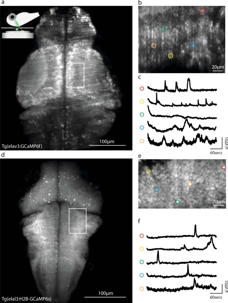
Whole-brain, neuron-level 3D imaging in larval zebrafish in vivo.
High-resolution images are recorded in steps of 8 u03bcm with an exposure time of 8u2009ms. A volume of 500 u03bcm * 300 u03bcm * 200 u03bcm, containing the entire brain, is recorded once every 0.3u20...
Extended Data Fig. 9
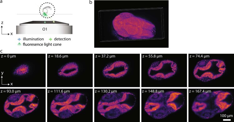
Imaging the whole brain of the zebrafish embryo.
( a ) show the orientation of the embryo mounted on the sample stage, with the head facing the primary objective (O 1 ). ( b ) 3D rendering of the zebrafish brain images. ( c ) XY slices of the brain ...
Extended Data Fig. 10
Data processing pipeline.
The 3D stacks from each view are initially in the x 1 u2019yz 1 u2019 and x 2 u2019yz 2 u2019 coordinates respectively. The stacks are then resampling to the sample (that is, xyz) coordinates. This pr...
Figure images are served from the NIH/NLM PubMed Central Open Access Subset or Europe PMC; copyright remains with the publishers and authors.
💬 Discussion
0 commentsNo comments yet. Be the first to start a discussion!
Leave a Comment