Abstract
AbstractMINimal fluorescence photon FLUXes (MINFLUX) nanoscopy, providing photon-efficient fluorophore localizations, has brought about three-dimensional resolution at nanometer scales. However, by using an intrinsic on–off switching process for single fluorophore separation, initial MINFLUX implementations have been limited to two color channels. Here we show that MINFLUX can be effectively combined with sequentially multiplexed DNA-based labeling (DNA-PAINT), expanding MINFLUX nanoscopy to multiple molecular targets. Our method is exemplified with three-color recordings of mitochondria in human cells.
🔬 Techniques
💻 Software
✨ Fluorophores
🧪 Sample Preparation
🔬 Cell Lines
🏭 Microscope Brands
🧪 Reagent Suppliers
💻 Software Details
💾 Data Repositories
🏛️ Research Organizations (ROR)
Affiliated research institutions:
📋 Methods
Cell lines
The genome-edited U2OS cell lines HMGA1 -rsEGFP2 (homozygous), Zyxin -rsEGFP2 (homozygous) and Vimentin -rsEGFP2 (heterozygous) were described in ref. 20 . The heterozygous TOMM70A -Dreiklang U2OS cell line was generated as described in ref. 20 . The homozygous NUP96 -mEGFP cell line U2OS-CRISPR- NUP96 -mEGFP clone no. 195 (300174) 21 and the NUP107 -mEGFP cell line HK-2xZFN-mEGFP-Nup107 (300676) 22 were purchased from CLS GmbH (CLS Cell Lines Service GmbH).
Cell culture
U2OS cells were cultivated in McCoy’s 5a medium (Thermo Fisher Scientific), supplemented with 100 U ml −1 penicillin, 100 μg ml −1 streptomycin, 1 mM Na-pyruvate and 10% (v/v) FBS (Invitrogen) at 37 °C, 5% CO 2 .
HeLa Kyoto cells
(HK-2xZFN-mEGFP-Nup107) were cultivated in DMEM, high glucose, GlutaMAX Supplement, pyruvate (Thermo Fisher Scientific), supplemented with 100 U ml −1 penicillin, 100 μg ml −1 streptomycin and 10% (v/v) FBS (Invitrogen) at 37 °C, 5% CO 2 .
Sample preparation
The cells were cultured for 1 day on cover slips (Marienfeld) or in eight-well chambered cover slips (ibidi) and fixed in prewarmed 8% formaldehyde in PBS for 10 min. Fixed cells were permeabilized with 0.5% (v/v) Triton X-100 in PBS for 5 min. NUP107-mEGFP cells were fixed in 2.4% formaldehyde in PBS for 30 min at room temperature and after fixation incubated with 0.1 M NH 4 Cl in PBS for 5 min. Then, NUP107-mEGFP cells were permeabilized with 0.25% (v/v) Triton X-100. Afterward, all cells were blocked in antibody incubation buffer (Massive Photonics) for roughly 30 min. The cells were incubated for 1 h with the MASSIVE-TAG-Q anti-GFP single domain antibody (Massive Photonics) or with the FluoTag-Q anti-GFP single domain antibody (conjugated with Alexa Fluor 647) (NanoTag Biotechnologies) in antibody incubation buffer (Massive Photonics) at a dilution of 1:100. The cells were then washed three times with 1× washing buffer (Massive Photonics). For multiplexing, the cells were fixed, permeabilized and blocked as described above. Afterward, the cells were incubated for 1 h at room temperature with primary antibodies against Mic60 (Proteintech) at a concentration of 1.235 µg ml −1 and ATP synthase subunit beta (Abcam) at a concentration of 5 µg ml −1 in antibody incubation buffer (Massive Photonics). After three washing steps with PBS, the cells were incubated with polyclonal secondary antibodies coupled to DNA-PAINT docking sites, targeting mouse and rabbit IgGs (Massive Photonics) at a dilution of 1:400 each and with MASSIVE-TAG-Q anti-GFP single domain antibody (Massive Photonics) at a dilution of 1:100. The cells were then washed three times with 1× washing buffer (Massive Photonics).
Show full methods section
Cell lines
The genome-edited U2OS cell lines HMGA1 -rsEGFP2 (homozygous), Zyxin -rsEGFP2 (homozygous) and Vimentin -rsEGFP2 (heterozygous) were described in ref. 20 . The heterozygous TOMM70A -Dreiklang U2OS cell line was generated as described in ref. 20 . The homozygous NUP96 -mEGFP cell line U2OS-CRISPR- NUP96 -mEGFP clone no. 195 (300174) 21 and the NUP107 -mEGFP cell line HK-2xZFN-mEGFP-Nup107 (300676) 22 were purchased from CLS GmbH (CLS Cell Lines Service GmbH).
Cell culture
U2OS cells were cultivated in McCoy’s 5a medium (Thermo Fisher Scientific), supplemented with 100 U ml −1 penicillin, 100 μg ml −1 streptomycin, 1 mM Na-pyruvate and 10% (v/v) FBS (Invitrogen) at 37 °C, 5% CO 2 .
HeLa Kyoto cells
(HK-2xZFN-mEGFP-Nup107) were cultivated in DMEM, high glucose, GlutaMAX Supplement, pyruvate (Thermo Fisher Scientific), supplemented with 100 U ml −1 penicillin, 100 μg ml −1 streptomycin and 10% (v/v) FBS (Invitrogen) at 37 °C, 5% CO 2 .
Sample preparation
The cells were cultured for 1 day on cover slips (Marienfeld) or in eight-well chambered cover slips (ibidi) and fixed in prewarmed 8% formaldehyde in PBS for 10 min. Fixed cells were permeabilized with 0.5% (v/v) Triton X-100 in PBS for 5 min. NUP107-mEGFP cells were fixed in 2.4% formaldehyde in PBS for 30 min at room temperature and after fixation incubated with 0.1 M NH 4 Cl in PBS for 5 min. Then, NUP107-mEGFP cells were permeabilized with 0.25% (v/v) Triton X-100. Afterward, all cells were blocked in antibody incubation buffer (Massive Photonics) for roughly 30 min. The cells were incubated for 1 h with the MASSIVE-TAG-Q anti-GFP single domain antibody (Massive Photonics) or with the FluoTag-Q anti-GFP single domain antibody (conjugated with Alexa Fluor 647) (NanoTag Biotechnologies) in antibody incubation buffer (Massive Photonics) at a dilution of 1:100. The cells were then washed three times with 1× washing buffer (Massive Photonics). For multiplexing, the cells were fixed, permeabilized and blocked as described above. Afterward, the cells were incubated for 1 h at room temperature with primary antibodies against Mic60 (Proteintech) at a concentration of 1.235 µg ml −1 and ATP synthase subunit beta (Abcam) at a concentration of 5 µg ml −1 in antibody incubation buffer (Massive Photonics). After three washing steps with PBS, the cells were incubated with polyclonal secondary antibodies coupled to DNA-PAINT docking sites, targeting mouse and rabbit IgGs (Massive Photonics) at a dilution of 1:400 each and with MASSIVE-TAG-Q anti-GFP single domain antibody (Massive Photonics) at a dilution of 1:100. The cells were then washed three times with 1× washing buffer (Massive Photonics).
Sample mounting and imaging buffer
For the stabilization of the samples during MINFLUX imaging, the samples were incubated with 100 µl of gold nanorod dispersion (A12-40-980-CTAB-DIH-1-25, Nanopartz Inc.) for 7 min, as described before 2 , 4 . To remove unbound nanorods, the samples were rinsed with PBS several times. For single-color DNA-PAINT imaging, aliquots (5 µM) of the DNA-PAINT imager strand conjugated to Atto 655 (Massive Photonics) were diluted in imaging buffer (Massive Photonics) (final concentrations indicated in Supplementary Table 1 ). Alternatively, for MINFLUX imaging of Alexa Fluor 647, standard STORM buffer containing 10 mM MEA (Sigma-Aldrich), 64 µg ml −1 catalase from bovine liver (Sigma-Aldrich), 0.4 mg ml −1 glucose oxidase from Aspergillus niger (Sigma-Aldrich), 50 mM Tris/HCl, 10 mM NaCl and 10% (w/v) glucose, pH 8.0 was used 23 . Cover slips were sealed with picodent twinsil (picodent) on cavity slides (Brand GmbH & CO KG). For multiplexing, eight-well chambered cover slips (ibidi) were used. After incubation with gold nanorod dispersion and washing as described above, aliquots (5 µM) of the DNA-PAINT imager strand (conjugated to Atto 655) (Massive Photonics) transiently binding to MASSIVE-TAG-Q anti-GFP single domain antibody were diluted in imaging buffer (final concentration 2 nM) (Massive Photonics) and added to the cells. After DNA-PAINT MINFLUX imaging, the cells were washed on the microscope stage five times with PBS and one time with imaging buffer (Massive Photonics). Subsequently, DNA-PAINT imager (conjugated to Atto 655) (Massive Photonics) transiently binding to the anti-rabbit IgG was diluted (final concentration 1 nM) and added. After recording of the second DNA-PAINT MINFLUX dataset this process was repeated and imager transiently binding to the anti-mouse IgG (final concentration 1 nM) was added.
MINFLUX measurements
The data were acquired on an Abberior MINFLUX microscope (Abberior Instruments) 4 using Imspector Software (v.16.3.11647M-devel-win64-MINFLUX, Abberior Instruments). For MINFLUX measurements, the Imspector MINFLUX sequence templates seqIIF (2D) and DefaultIIF3D (3D) provided and optimized by the manufacturer for samples with the dye Alexa Fluor 647 were used ( MINFLUX sequences ). Cells were identified and placed in the focus using the 488 nm confocal scan of the microscope. If necessary, the persistent binding–unbinding activity of imager strands was verified in the 642-nm confocal scan. Before starting a MINFLUX measurement, the stabilization system of the microscope was activated. Measurements were conducted with a stabilization precision of typically below 1 nm. A region of interest was selected in the confocal scan image and laser power and pinhole size were adjusted in the software (indicated pinhole sizes in AU refer to the emission maximum of Atto 655 at 680 nm). For MINFLUX measurements of Alexa Fluor 647 (Fig. 1e ) a laser power of 12 µW in the first iteration and a pinhole diameter of 0.6 AU were used. Finally, the MINFLUX measurement was started in the region of interest.
Quantification measurement series
In a measurement series ( Supplementary Notes ) one of the experimental parameters, namely laser power, pinhole size or imager concentration, was varied, while the other parameters were kept constant. Within one measurement series, we recorded 2D MINFLUX images of labeled nuclear pores close to the cover slip and kept the image size and the recording time (1 h) constant. All images were taken with the same MINFLUX iteration sequence. Multiple regions (1 × 1 µm) of the lower envelope of one nucleus were measured. Each region was imaged with a different experimental parameter. Each measurement series was repeated three times on different days with fresh samples. Daily alignment of the MINFLUX nanoscope The shape of the intensity pattern ('donut') for fluorescence excitation was evaluated using immobilized fluorescent beads (GATTA-BEAD R, Gattaquant GmbH) and if necessary optimized by changing the spatial light modulator parameters. Additionally, the position of the pinhole was adjusted so that the confocal detection matched the excitation volume. If during measurement series more than one pinhole size was used, all pinhole positions were determined before starting the measurement series. The pinhole position was then adjusted before each measurement.
MINFLUX data analysis
Data export Each MINFLUX measurement was exported using Imspector Software (Abberior Instruments). The exported files contained a collection of recorded parameters for all valid localizations and also included discarded nonvalid localization attempts. Additional information of the measurement (laser power and so on) was stored manually. Both were imported in a custom analysis script written in MATLAB (R2018b) to calculate the following quantification parameters in an automated manner.
Quantification
For all calculations, only data of the last MINFLUX iterations (in two dimensions fourth, in three dimensions nineth, after one prelocalization iteration), which were also identified as valid (exported parameter VLD = 1), were used. The first quantification parameter to be calculated was the time that passed between the localization of two valid events, in short, the time between events or t btw . An emitting molecule is usually localized by the microscope several times in direct succession by repeating the last two MINFLUX iterations. These successive localizations are assigned to the same event via the same trace ID (exported parameter TID). Moreover, for each individual localization the time at which its localization process started was saved (exported parameter TIM). This allowed the determination of the start and end time of each molecule binding event. Each event (TID) was terminated after a predefined number of nonvalid localization attempts. The time of the first final nonvalid localization attempt was defined as the end time of the molecule binding event. Finally, t btw was calculated as the time difference between two consecutive valid events by subtracting the end time of the first molecule from the start time of the second molecule. For each measurement, the median of the first 100 events was determined as t btw . Time between molecule binding events t btw calculated from the exported measurement parameters Saved localization attempts are depicted as colored rectangles, arranged in order of their appearance. Valid localization attempts were saved with the exported parameter VLD = 1 and are shown as green, while the nonvalid localization attempts were saved with VLD = 0 and are shown in yellow. The beginning of a localization attempt is saved as a time stamp (exported parameter TIM), here shown simplified as dimensionless values from 1 to 10. Localization events belonging to the same molecule have the same trace ID (exported parameter TID). Here, the time between the two consecutive valid molecules is calculated as the time difference between the start of molecule 4 (TIM = 7) and the end of molecule 2 (TIM = 5). The second quantification parameter was the background emission frequency ( f bg ). The f bg is continuously estimated by the MINFLUX microscope between valid events and is used by the system to identify emission events and to correct emission frequencies of localization events. The third quantification parameter was the CFR. The CFR is the ratio of the effective emission frequency at the central position of the MINFLUX excitation pattern over the mean effective emission frequency over all outer positions and defined as documentclass[12pt]{minimal} usepackage{amsmath} usepackage{wasysym} usepackage{amsfonts} usepackage{amssymb} usepackage{amsbsy} usepackage{mathrsfs} usepackage{upgreek} setlength{oddsidemargin}{-69pt} begin{document}$${{{mathrm{CFR}}}} = f_{{{{mathrm{eff}}}}}({{{mathrm{central}}}},{{{mathrm{position}}}})/f_{{{{mathrm{eff}}}}}({{{mathrm{outer}}}},{{{mathrm{positions}}}})$$end{document} CFR = f eff ( central position ) / f eff ( outer positions ) . The effective frequencies f eff are the measured emission frequencies above a background automatically determined by the system. The value of the CFR is regarded as a quality measure for the localization process. For each measurement, the median CFR of all valid localizations in the last iteration was determined. The CFR is calculated directly by the microscope software and is also used for filtering in early iterations (exported parameter CFR). It therefore directly influences the measurement 4 . To estimate the localization precision of a measurement as the third quantification parameter, the standard deviation σ r was calculated for each molecule (at least five localizations with the same exported parameter TID) as documentclass[12pt]{minimal} usepackage{amsmath} usepackage{wasysym} usepackage{amsfonts} usepackage{amssymb} usepackage{amsbsy} usepackage{mathrsfs} usepackage{upgreek} setlength{oddsidemargin}{-69pt} begin{document}$$sigma _r = sqrt {left( {sigma _x^2 + sigma _y^2} right)/2}$$end{document} σ r = σ x 2 + σ y 2 / 2 with the standard deviations of the x and y coordinates as determined by the microscope (exported parameter POS). The median σ r represents the stated localization precision. The combined localization precision was estimated as documentclass[12pt]{minimal} usepackage{amsmath} usepackage{wasysym} usepackage{amsfonts} usepackage{amssymb} usepackage{amsbsy} usepackage{mathrsfs} usepackage{upgreek} setlength{oddsidemargin}{-69pt} begin{document}$$sigma _{rmathrm{c}} = leftlangle {leftlangle {sigma _r} rightrangle /surd n} rightrangle _n$$end{document} σ r c = σ r / √ n n , that is the weighted average of the average single localization precision σ r divided by √ n and weighted by the occurrence of n being the number of single localizations with the same TID. The precision in the z direction is often different from x and y , therefore we separately computed the combined localization precision in z: documentclass[12pt]{minimal} usepackage{amsmath} usepackage{wasysym} usepackage{amsfonts} usepackage{amssymb} usepackage{amsbsy} usepackage{mathrsfs} usepackage{upgreek} setlength{oddsidemargin}{-69pt} begin{document}$$sigma _{zc} = leftlangle {leftlangle {sigma _z} rightrangle /surd n} rightrangle _n$$end{document} σ z c = σ z / √ n n . CFR simulation The CFR is a parameter that is directly calculated during image acquisition by the MINFLUX software. To understand and judge the CFR values from the experimental results we simulated the CFR dependency on pinhole size and imager strand concentration for a molecule that is located at the center of the MINFLUX targeted coordinate pattern (TCP) with background contributions included ( Supplementary Notes and Supplementary Fig. 3 ). The excitation PSF documentclass[12pt]{minimal} usepackage{amsmath} usepackage{wasysym} usepackage{amsfonts} usepackage{amssymb} usepackage{amsbsy} usepackage{mathrsfs} usepackage{upgreek} setlength{oddsidemargin}{-69pt} begin{document}$$h_{{{{mathrm{exc}}}}}(x,y,z)$$end{document} h exc ( x , y , z ) in shape of a 2D donut was determined via fast focus field calculations 24 for high numerical apertures and using realistic values for the objective lens properties as well as an excitation wavelength λ exc = 642 nm. The confocal detection PSF h det ( x , y , z ) was calculated 25 for a detection wavelength of λ exc = 680 nm. We then calculated the resulting effective PSF documentclass[12pt]{minimal} usepackage{amsmath} usepackage{wasysym} usepackage{amsfonts} usepackage{amssymb} usepackage{amsbsy} usepackage{mathrsfs} usepackage{upgreek} setlength{oddsidemargin}{-69pt} begin{document}$$h_{{{{mathrm{eff}}}},i} = h_{{{{mathrm{exc}}}},i} h_{{{{mathrm{det}}}}}$$end{document} h eff , i = h exc , i h det for each exposure i by shifting h exc to the according exposure position in the MINFLUX TCP while keeping the confocal detection h det centered. The background contribution due to diffusing imager strand was calculated in two steps. The resulting background intensity B i in the effective excitation volume was calculated as documentclass[12pt]{minimal} usepackage{amsmath} usepackage{wasysym} usepackage{amsfonts} usepackage{amssymb} usepackage{amsbsy} usepackage{mathrsfs} usepackage{upgreek} setlength{oddsidemargin}{-69pt} begin{document}$$B_iapprox {int}_{!x,y,z} {h_{{{{mathrm{eff}}}},i}} left( {x,y,z} right) times c_{{{{mathrm{imager}}}}}dxdydz$$end{document} B i ≈ ∫ x , y , z h eff , i x , y , z × c imager d x d y d z for each exposure. For the CFR calculation, we assumed that the central donut exposure of the MINFLUX TCP is placed directly on the molecule, chosen here as the origin. In the case of a perfect donut zero, this leads to a detected emitter intensity of I center = 0 for this exposure. The signal intensity detected at different exposures is calculated as documentclass[12pt]{minimal} usepackage{amsmath} usepackage{wasysym} usepackage{amsfonts} usepackage{amssymb} usepackage{amsbsy} usepackage{mathrsfs} usepackage{upgreek} setlength{oddsidemargin}{-69pt} begin{document}$$I_iapprox h_{{{{mathrm{eff}}}},i}(0,0,0)$$end{document} I i ≈ h eff , i ( 0 , 0 , 0 ) . Correcting for the different total time spent in the inner and outer exposures, the mean background intensity documentclass[12pt]{minimal} usepackage{amsmath} usepackage{wasysym} usepackage{amsfonts} usepackage{amssymb} usepackage{amsbsy} usepackage{mathrsfs} usepackage{upgreek} setlength{oddsidemargin}{-69pt} begin{document}$$bar B_{{{{mathrm{outer}}}}}$$end{document} B ¯ outer and mean signal intensity documentclass[12pt]{minimal} usepackage{amsmath} usepackage{wasysym} usepackage{amsfonts} usepackage{amssymb} usepackage{amsbsy} usepackage{mathrsfs} usepackage{upgreek} setlength{oddsidemargin}{-69pt} begin{document}$$bar I_{{{{mathrm{outer}}}}}$$end{document} Ī outer was calculated for the outer exposures ( documentclass[12pt]{minimal} usepackage{amsmath} usepackage{wasysym} usepackage{amsfonts} usepackage{amssymb} usepackage{amsbsy} usepackage{mathrsfs} usepackage{upgreek} setlength{oddsidemargin}{-69pt} begin{document}$$i ne 1$$end{document} i ≠ 1 ). Therefore, we were able to calculate the CFR as documentclass[12pt]{minimal} usepackage{amsmath} usepackage{wasysym} usepackage{amsfonts} usepackage{amssymb} usepackage{amsbsy} usepackage{mathrsfs} usepackage{upgreek} setlength{oddsidemargin}{-69pt} begin{document}$${{{mathrm{CFR}}}} = frac{{B_{{mathrm{center}}} + I_{{mathrm{center}}}}}{{leftlangle {bar B_{{mathrm{outer}}} + bar I_{{mathrm{outer}}}} rightrangle }}$$end{document} CFR = B center + I center B ¯ outer + Ī outer for different scenarios. We repeated the calculations for different concentrations c , adapted the pinhole size when determining h det and used different values for the TCP diameter L .
Sample drift correction
Sample drift was corrected from the extracted molecule event position and time pairs by dividing the events into overlapping time windows of approximately 2,000 events per window, and generating a 2D or 3D rendered MINFLUX image (placing a Gaussian peak with standard deviation sigma of 2 nm at each estimated molecule position) and calculating 2D or 3D cross-correlations between images from different time windows. The center of the cross-correlation peak was fitted with a Gaussian function and its offset relative to the center of the cross-correlation presented the spatial sample shift between the corresponding time points. The drift curve that fulfilled all possible sample drift estimations for all possible time window pairs was estimated in a least squares sense. A smooth (cubic spline) interpolation of the estimated drift curve for all time points of all events was then subtracted from the molecule coordinates. FRC xy calculations For the determination of the FRC shown in Supplementary Table 1 and Extended Data Fig. 3 we implemented the algorithm described in ref. 19 . In brief, a dataset of combined localizations (only x and y positions) was divided into two statistically independent subsets resulting in two subimages, each containing 50% of the combined localizations of the original dataset. Then, the average correlation of the Fourier transform of these subimages was calculated on rings of constant spatial frequency. The inverse of the spatial frequency at which the FRC drops below one-seventh was taken as a measure of the FRC resolution. We used combined localizations instead of single localizations for the estimation of the FRC resolution, because for single localizations the FRC is dominated by the large number of repeated localizations during one binding event and the calculated FRC resolution is then strictly proportional to the single localization precision. To obtain a more robust result, the random division into subsets was repeated several times and the obtained FRC resolutions for each division were averaged.
Image rendering in two dimensions
All valid localization events were rendered using Imspector Software and displayed as 2D histograms with the bin size 4 nm (Fig. 1a–f ) and 1 nm (Fig. 1f , close-up). Image rendering in three dimensions Each MINFLUX measurement was exported with Imspector Software. The data were drift corrected ( Sample drift correction ) and the z position was scaled with the scaling factor 0.7 (ref. 3 ). A rendering of the resulting localizations where each localization was replaced by a Gaussian peak with sigma 5 nm was imported into the Imaris Software (Imaris x64, v.9.7.2, Bitplane AG). The data were displayed as a blend volume rendition. MINFLUX sequences The MINFLUX microscope’s data acquisition is controlled by a set of parameters that are specified within a text file (see seqIIF.json and seqDefaultIIF3d.json in the Supplementary Data ). The set of parameters defines a sequence that controls the iterative zooming in on single molecule events and was provided and optimized by the manufacturer for samples with the dye Alexa Fluor 647. The MINFLUX iteration process is described in ref. 4 . In two dimensions, four iterations plus one prelocalization iteration were performed. In three dimensions, nine iterations plus one prelocalization iteration were performed. In the last iteration an L of 40 nm was used. Key parameters of the 2D iteration sequence include: TCP parameter L (nm) Photon limit (minimal photon count) Dwell time (ms) CFR limit Laser power factor Prelocalization 160 ≥1 Off 1 Iteration 1 288 150 ≥1 0.5 1 Iteration 2 151 100 ≥1 Off 2 Iteration 3 76 100 ≥1 0.8 4 Iteration 4 40 150 ≥1 Off 6 Supplementary software and data An additional software package is provided with the manuscript (10.5281/zenodo.6563100) to facilitate reanalysis of the MINFLUX localization data. The package is written in MATLAB and contains experimental localization data of all recorded DNA-PAINT MINFLUX datasets, which are shown in this publication. The software applies analysis steps such as drift correction, precision estimation, as well as CFR and FRC calculations on each dataset. Availability of materials U2OS cells lines HMGA1-rsEGFP2, Zyxin-rsEGFP2, Vimentin-rsEGFP2 and TOMM70A-Dreiklang are available from the corresponding author upon reasonable request. All other materials are commercially available.
Statistics and reproducibility
All experiments in this paper were performed independently at least three times and yielded similar results. Reporting summary Further information on research design is available in the Nature Research Reporting Summary linked to this article.
Availability of materials U2OS cells lines HMGA1-rsEGFP2, Zyxin-rsEGFP2, Vimentin-rsEGFP2 and TOMM70A-Dreiklang are available from the corresponding author upon reasonable request. All other materials are commercially available.
Online content Any methods, additional references, Nature Research reporting summaries, source data, extended data, supplementary information, acknowledgements, peer review information; details of author contributions and competing interests; and statements of data and code availability are available at 10.1038/s41592-022-01577-1.
Supplementary information Supplementary Information Supplementary Table 1, Notes and Figs. 1–4.
Reporting Summary Peer Review File Supplementary Data
MINFLUX sequences that control parameters of the MINFLUX measurement (seqIIF.json and seqDefaultIIF3d.json).
Supplementary information The online version contains supplementary material available at 10.1038/s41592-022-01577-1.
📊 Figures
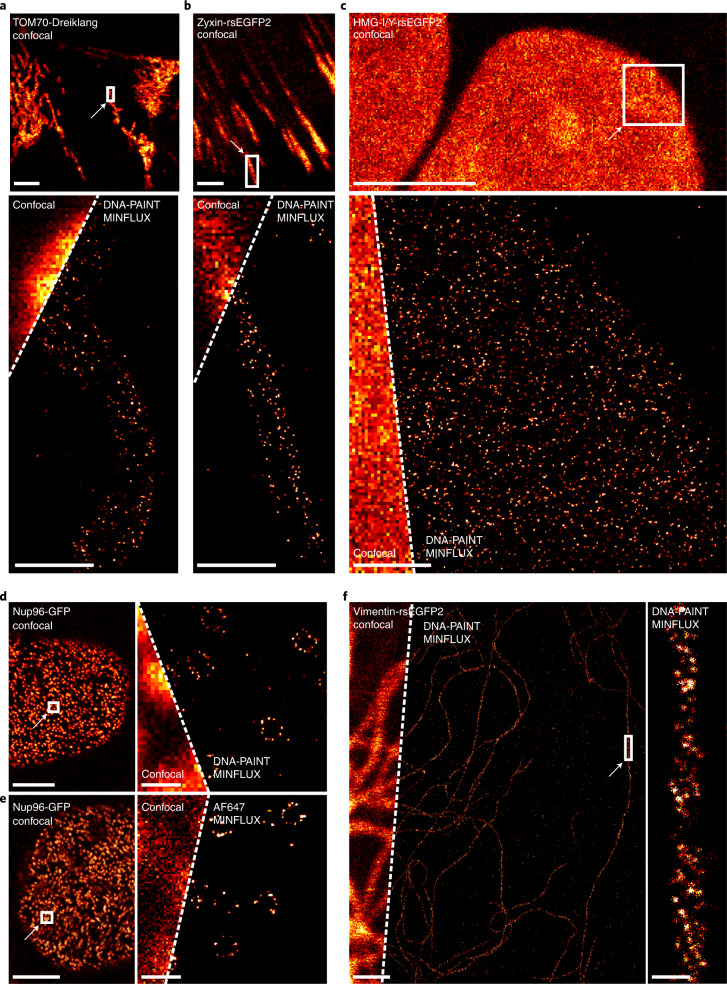
Fig. 1
2D DNA-PAINT MINFLUX imaging.
a u2013 f , Genome-edited cell lines expressing translational fusions with a fluorescent protein from the respective native genomic loci, as indicated (TOM70-Dreiklang ( a ), Zyxin-rsEGFP2 ( b ), HMG-...
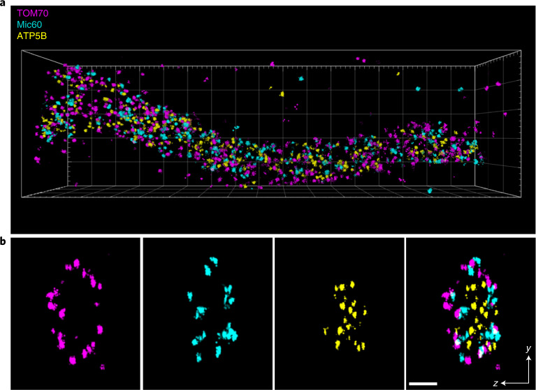
Fig. 2
3D DNA-PAINT MINFLUX multiplexing.
U2OS TOM70-Dreiklang cells were fixed and immuno-labeled with an anti-GFP nanobody and anti-Mic60 and anti-ATP5B synthase antibodies. MINFLUX recordings of the three proteins were performed sequential...
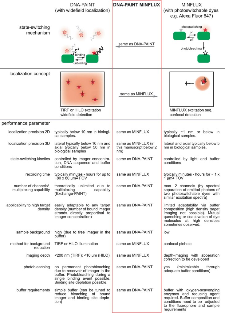
Extended Data Fig. 1
Comparison of current DNA-PAINT, DNA-PAINT MINFLUX and MINFLUX implementations.
The three techniques are compared with respect to their state-switching mechanisms, their localization concepts and key performance parameters.
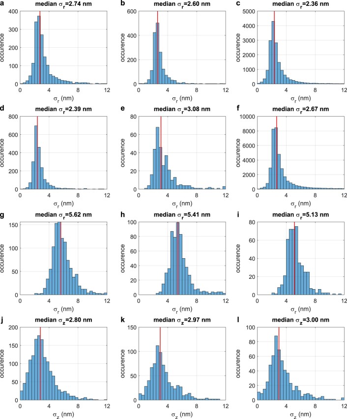
Extended Data Fig. 2
Histograms of the localization precisions in Fig. 1 and Fig. 2 .
Blue columns represent the frequencies of localization precisions in the given dataset ( a : Fig. 1a ; b : Fig. 1b ; c : Fig. 1c ; d : Fig. 1d ; e : Fig. 1e ; f : Fig. 1f ; g : Fig. 2 TOM70 u03c3 r ; ...
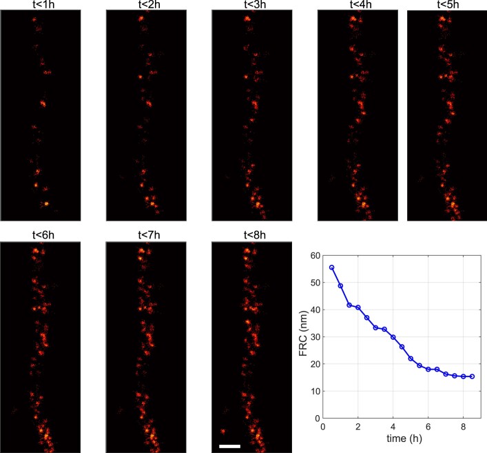
Extended Data Fig. 3
The labeling coverage, but not insufficient sampling during a MINFLUX recording, limits the density of localized molecules.
The individual panels show all recorded localizations in the indicated time intervals. The full field of view of the 8-hour data set is shown in Fig. 1f . The FRC resolution was calculated using all d...
Figure images are served from the NIH/NLM PubMed Central Open Access Subset or Europe PMC; copyright remains with the publishers and authors.
💬 Discussion
0 commentsNo comments yet. Be the first to start a discussion!
Leave a Comment