Abstract
SummaryIn biological fluorescence microscopy, image contrast is often degraded by a high background arising from out of focus regions of the specimen. This background can be greatly reduced or eliminated by several modes of thick specimen microscopy, including techniques such as 3‐D deconvolution and confocal. There has been a great deal of interest and some confusion about which of these methods is ‘better’, in principle or in practice. The motivation for the experiments reported here is to establish some rough guidelines for choosing the most appropriate method of microscopy for a given biological specimen. The approach is to compare the efficiency of photon collection, the image contrast and the signal‐to‐noise ratio achieved by the different methods at equivalent illumination, using a specimen in which the amount of out of focus background is adjustable over the range encountered with biological samples. We compared spot scanning confocal, spinning disk confocal and wide‐field/deconvolution (WFD) microscopes and find that the ratio of out of focus background to in‐focus signal can be used to predict which method of microscopy will provide the most useful image. We also find that the precision of measurements of net fluorescence yield is very much lower than expected for all modes of microscopy. Our analysis enabled a clear, quantitative delineation of the appropriate use of different imaging modes relative to the ratio of out‐of‐focus background to in‐focus signal, and defines an upper limit to the useful range of the three most common modes of imaging.
🔬 Techniques
🔭 Microscopes
💻 Software
✨ Fluorophores
🧪 Sample Preparation
🏭 Microscope Brands
🧪 Reagent Suppliers
📷 Detectors
🔎 Objectives
💻 Software Details
🏛️ Research Organizations (ROR)
Affiliated research institutions:
📋 Methods
Background solution AlexaFluor488 hydroxylamine (Molecular Probes #A30269) was dissolved in dry dimethylformamide to give a 10 mM stock solution which was stored at −20°C. Five μL of this stock was mixed with 0.5 mL of 10 mM glucose in 10 mM bicine pH 8.4 (final 100 μM fluorescent glucose, in ∼10 mM nonfluorescent glucose) and incubated at room temp for 1 h. NaN 3 was added to 10 mM and EDTA to 0.1 mM as preservatives, and the solution was frozen in aliquots at −20°C. Dilutions of this stock were made with 10 mM glucose, 10 mM bicine pH 8.4, 10 mM NaN 3 , 0.1 mM EDTA to prepare background solutions with concentrations of AlexaFluor488 glucose lower than 100 μM. Beads A total of 0.4 mL red fluorescent (580 ex/605 em) amine modified latex microspheres, 0.21 μm diameter (Molecular Probes #F8763; 2% solids; ∼3.9 × 10 12 /mL; 5.3 μeq amine residues/mL) was washed twice with water, then suspended in 0.8 mL of 0.02% Tween 20, 12.5 mM NaHCO 3 pH 8.3. Fluorescein succinimidyl ester (Molecular Probes #F6130, 1.6 mg in 0.2 mL of DMSO) was added in 20 μL aliquots to the bead suspension with vigorous stirring. After rotation for 1 h at room temperature, 0.8 mL 1 M glycine in 0.1 M NaHCO 3 , was added, followed by another hour of rotation, addition of bovine serum albumin (BSA) to a final concentration of 2%, rotation for 15 min, centrifugation at ∼10 000 × g for 3 min, resuspension and washing three times with 0.02% Tween 20, 1% BSA, 10 mM TrisCl pH8.5. The bead suspension was allowed to stand overnight, then centrifuged and resuspended in 1 mL 10 mM TrisCl pH8.5 (no BSA, no Tween20) and stored at 4 °C until use. The amount of fluorescein in a 300-fold diluted bead suspension (=2×10 −8 M) was estimated by comparison of the green fluorescence of a washed bead suspension in 10 mM bicine pH 8.4 with dilutions in the same buffer of a 50.7 μM solution of fluorescein (Molecular Probes # F36915 NIST traceable fluorescein standard), fluorescence measured with 490 nm excitation, 520 nm emission, 10 nm bandpass. The number of beads in the same diluted bead suspension (=5.8 × 10 9 /mL) was estimated by comparison of its red fluorescence with dilutions of the original stock bead suspension (3.9 × 10 12 beads/mL according to the manufacturer), fluorescence measured with 580 nm excitation, 605 nm emission, 10 nm bandpass. The results of those two comparisons were then used to calculate the apparent number of fluorescein molecules per bead (=2070). Fluorescence measurements were carried out in 3 mL quartz cuvettes using a Hitachi Model F2000 fluorescence spectrophotometer. The beads were also characterized by flow cytometry using a Becton–Dickinson FACSCalibur instrument, with 488 nm excitation, and fluorescence detection in three channels: 515–545 nm, 564–606 nm and >670 nm. This analysis yielded an estimate of fluorescein per bead equivalent to 2100 molecules of fluorescein in solution, in excellent agreement with the value measured by spectrophotometer. The coefficient of variation (CV) of the fluorescein signal in the flow cytometer was 16%, which is entirely accounted for by the Poisson statistical variation of the estimated number of photons ( Shapiro, 2003 ) detected per bead in the fluorescein channel, ∼40. Thus the fluctuation in fluorescein content per bead must be substantially less than 16%, but it is not possible to estimate the heterogeneity any more precisely than this.
Show full methods section
Background solution AlexaFluor488 hydroxylamine (Molecular Probes #A30269) was dissolved in dry dimethylformamide to give a 10 mM stock solution which was stored at −20°C. Five μL of this stock was mixed with 0.5 mL of 10 mM glucose in 10 mM bicine pH 8.4 (final 100 μM fluorescent glucose, in ∼10 mM nonfluorescent glucose) and incubated at room temp for 1 h. NaN 3 was added to 10 mM and EDTA to 0.1 mM as preservatives, and the solution was frozen in aliquots at −20°C. Dilutions of this stock were made with 10 mM glucose, 10 mM bicine pH 8.4, 10 mM NaN 3 , 0.1 mM EDTA to prepare background solutions with concentrations of AlexaFluor488 glucose lower than 100 μM. Beads A total of 0.4 mL red fluorescent (580 ex/605 em) amine modified latex microspheres, 0.21 μm diameter (Molecular Probes #F8763; 2% solids; ∼3.9 × 10 12 /mL; 5.3 μeq amine residues/mL) was washed twice with water, then suspended in 0.8 mL of 0.02% Tween 20, 12.5 mM NaHCO 3 pH 8.3. Fluorescein succinimidyl ester (Molecular Probes #F6130, 1.6 mg in 0.2 mL of DMSO) was added in 20 μL aliquots to the bead suspension with vigorous stirring. After rotation for 1 h at room temperature, 0.8 mL 1 M glycine in 0.1 M NaHCO 3 , was added, followed by another hour of rotation, addition of bovine serum albumin (BSA) to a final concentration of 2%, rotation for 15 min, centrifugation at ∼10 000 × g for 3 min, resuspension and washing three times with 0.02% Tween 20, 1% BSA, 10 mM TrisCl pH8.5. The bead suspension was allowed to stand overnight, then centrifuged and resuspended in 1 mL 10 mM TrisCl pH8.5 (no BSA, no Tween20) and stored at 4 °C until use. The amount of fluorescein in a 300-fold diluted bead suspension (=2×10 −8 M) was estimated by comparison of the green fluorescence of a washed bead suspension in 10 mM bicine pH 8.4 with dilutions in the same buffer of a 50.7 μM solution of fluorescein (Molecular Probes # F36915 NIST traceable fluorescein standard), fluorescence measured with 490 nm excitation, 520 nm emission, 10 nm bandpass. The number of beads in the same diluted bead suspension (=5.8 × 10 9 /mL) was estimated by comparison of its red fluorescence with dilutions of the original stock bead suspension (3.9 × 10 12 beads/mL according to the manufacturer), fluorescence measured with 580 nm excitation, 605 nm emission, 10 nm bandpass. The results of those two comparisons were then used to calculate the apparent number of fluorescein molecules per bead (=2070). Fluorescence measurements were carried out in 3 mL quartz cuvettes using a Hitachi Model F2000 fluorescence spectrophotometer. The beads were also characterized by flow cytometry using a Becton–Dickinson FACSCalibur instrument, with 488 nm excitation, and fluorescence detection in three channels: 515–545 nm, 564–606 nm and >670 nm. This analysis yielded an estimate of fluorescein per bead equivalent to 2100 molecules of fluorescein in solution, in excellent agreement with the value measured by spectrophotometer. The coefficient of variation (CV) of the fluorescein signal in the flow cytometer was 16%, which is entirely accounted for by the Poisson statistical variation of the estimated number of photons ( Shapiro, 2003 ) detected per bead in the fluorescein channel, ∼40. Thus the fluctuation in fluorescein content per bead must be substantially less than 16%, but it is not possible to estimate the heterogeneity any more precisely than this.
Test specimens
To prepare bead specimens for imaging, 10 μL of bead suspension diluted 1:100 with dry EtOH was spread on a 22 mm #1.5 cover slip and allowed to air-dry. Twenty-five microlitres background solution was pipetted into a well formed using a Secure-Seal spacer (Molecular Probes #S24735). The cover slip with attached beads was inverted on this well of solution, pressed to make a firm seal and the edges of the cover slip were further sealed to the slide using nail polish. A slide with a thin layer of fluorophore was prepared using fluorescein coupled to BSA. Fifty microlitres 10% BSA in water was mixed with 50 μL 0.1 M NaHCO 3 pH 8.8 and ∼ 1 mg fluorescein succinimidyl ester (Molecular Probes #F6130) in 10 μL DMSO. After 1 h at room temperature the labelled protein was separated from free dye with a G25-Sephadex spin column. Five microlitres of labelled protein was spread evenly on a clean 22 × 22 mm cover slip, then rinsed with cold acetone. The cover slip was air-dried, the protein layer was fixed with 10% formaldehyde in PBS for 30 min, rinsed twice with 10 mM bicine pH 8.4, and mounted over a thin layer of the same buffer.
Microscopy
Images were collected on a variety of microscopes. In each case, the objective lens giving the brightest image was used and other optical components were chosen to give a pixel size of ∼0.1 μm. In all cases, the refractive index of the immersion oil was carefully selected empirically to minimize spherical aberration. In the WF microscopes, the field stop was set to a diameter just slightly greater than the field of view of the camera. In the confocal microscopes, preliminary measurements established the range over which emitted fluorescence increased linearly with illumination irradiance (i.e. no significant depletion of the ground-state population). Linearity of AOTF response was established independently of fluorescence yield by measuring excitation light reflected from a mirror at various AOTF settings. The confocality of confocal microscopes is dramatically affected by lateral and axial chromatic aberration. To compensate for this, all spot scanning systems include an adjustable ‘collimator’ lens that attempts to make the focal position for excitation wavelengths identical to the focal position for emission wavelengths. When the system is truly ‘confocal’, the light collected by a pinhole with diameter equivalent to one Airy disk (image plane) should be ∼70% of the total light that could be collected from a diffraction limited spot ( Sandison et al. , 1995a ). For spot scanning confocals, measurements were made of image intensity versus pinhole size to check that the expected plateau occurs at just beyond 1 Airy disk diameter, and re-alignment was carried out as necessary. For each microscope, two types of data were collected: (1) multiple sequential images of the same field of view for measuring the rate of photobleaching and (2) 3-D stacks of optical sections with two excitation/emission wavelengths for intensity measurements on single beads. Photobleaching measurements utilized specimens with no AlexaFluor488 glucose in the background solution. Fading of fluorescence in the green channel was recorded over time, at several levels of illumination irradiance. Small stacks of optical sections were acquired from fields having an appropriate density of well-separated single beads, using at least four different illumination irradiance/exposure time combinations for each specimen. Suitable regions were chosen by observation of the red fluorescence channel. In initial experiments, images were collected at a single visually identified focal plane, but it was found that variations in focus between different beads across the field of view was a large source of noise. Accordingly, all of the data presented here was acquired as 3-D stacks of three or five focal planes separated by 0.1 or 0.2 μm in z . For the fluorescein/AlexaFluor488 image (‘green channel’, 488 nm excitation, 500–550 nm emission), illumination irradiance and exposure times were different for specimens with different background fluorophore concentration, whereas the illumination condition for the ‘red channel’ images was the same for all specimens on a given microscope. Zeiss LSM510 (spot scanning confocal) Plan-Neofluar 1.3 numerical aperture (NA) 40× or 1.45 NA 100× objective lens; green channel: 488 nm argon laser excitation, 500–550 nm emission; red channel: 543 nm HeNe laser excitation, >580 nm longpass emission; pixel size 0.1 μm; z -increment 0.2 μm; pinhole size 1.0 or 0.5 Airy disk units; pixel dwell time 1.28 μs; illumination irradiance set by laser tube current, which was held at 30% of maximum, and an acousto-optical tunable filter (AOTF; 0.5–3% used for these experiments) Leica TCS SP2 AOBS (spot scanning confocal) A 63× PlanApo CS 1.4 NA objective lens; green channel: 488 nm laser excitation, 500–550 nm emission; red channel: 561 nm laser excitation, >580 nm longpass emission; pixel dwell time 2.5 μs; pixel size 0.1 μm; z -increment 0.2 μm; pinhole size 1.0 or 0.5 Airy disk unit. Illumination irradiance set by analogue laser tube current control (held at ‘Low’) and an AOTF. Olympus FV1000 (spot scanning confocal) A 60× PlanApo 1.42 NA objective lens; green channel: 488 nm argon laser excitation, 500–550 nm emission; red channel: 543 nm HeNe laser excitation, >580 nm longpass emission; pixel size 0.1 μm; pinhole size 1 Airy disk unit; pixel dwell time 2 μs. Illumination irradiance set by laser tube current control (set to its minimum value) and an AOTF. DeltaVision Spectris (WFD) Two different similarly equipped versions of this system were employed. The results were not significantly different; data from only one is reported here. Olympus IX70 base; 100× PlanApo 1.4 NA objective lens; Chroma Sedat Quad ET filter set #86000; green channel: 480–500 nm excitation, 507–543 nm emission; red channel: 543–568 nm excitation, 579–631 nm emission; CoolSnap HQ CCD camera (12-bit digitization, 6.4 μm pixels, full well capacity 18 000 e − , read noise 6 e − rms; quantum efficiency (QE) ∼ 60% at 525 nm); 2 × 2 binning, image pixel size 0.13 μm in xy , 0.2 μm in z . Illumination irradiance controlled by software selectable ND filters (1, 3, 10, 32, 50, 100%T). Exposure times ranged from 80 to 500 msec. The illumination field stop was set to a diameter ∼30% greater than the field of view of the CCD. Yokogawa CSU-10 (spinning disk confocal) Three versions of the spinning disk confocal using the Yokogawa CSU-10 scanhead were evaluated: Nikon TE2000U base, 100× 1.4 NA PlanApo objective lens. A Coherent 2.5 W ArKr laser and an AOTF were used for illumination and excitation wavelength selection (Prairie Technologies, Middleton, WI). A triple bandpass polychromatic mirror (Chroma # 53055) was used with single bandpass excitation and emission filters; green channel: 488 nm excitation, 500–550 nm emission; red channel: 568 nm excitation, 590–650 nm emission. Images were collected with a Hamamatsu ORCA-ER (12-bit digitization, 6.4 μm pixels, full well capacity 18 000 e − , read noise 8 e − rms; QE ∼70% at 525 nm) and MetaMorph software, using 2 × 2 binning, image pixel size 0.13 μm. Illumination irradiance control set by AOTF. Exposure times 300 to 2000 msec. Nikon TE2000U base, 100× 1.4 NA PlanApo objective lens. A Melles-Griot 100 mW ArKr laser and Sutter filter wheels were used for illumination and excitation wavelength selection. A triple bandpass polychromatic mirror (Chroma # 53055) was used with single bandpass excitation and emission filters; green channel: 488 nm excitation, 500–550 nm emission; red channel: 568 nm excitation, 590–650 nm emission. Images were collected with a Hamamatsu ORCA-ER (12-bit digitization, 6.4 μm pixels, full well capacity 18 000 e-, read noise 8 e- rms; QE ∼ 70% at 525 nm) and MetaMorph software, using 2 × 2 binning, image pixel size 0.13 μm. Illumination irradiance set by analogue tube current dial (held at ‘high’ or ‘low’). Exposure times from 75 to 8000 msec Nikon TE2000E base, 100× 1.45 PlanApo TIRF objective lens; Melles-Griot 50 mW ArKr gas laser; dual band-pass dichromatic mirror used with single wavelength excitation and single bandpass emission filter; green channel: 488 nm excitation, 500–550 nm emission; red channel: 568 nm excitation, 585–629 nm emission; Hamamatsu ORCA II ER camera, 14-bit digitization, 6.4 μm pixels, full well capacity 40 000 e − at 2 × 2 binning, read noise 4e − rms; QE ∼ 70% at 525 nm; image pixel size 0.13 μm. Illumination irradiance set by analogue tube current dial (held at ‘8’). Exposure times 200 to 3000 msec.
Detector calibration
For each microscope system, the proportionality factor ( g ) relating image intensity values (grey levels) to the apparent number of photons detected was measured. The value was obtained from a graph of variance versus mean intensity for a set of images. To determine image variance, a pair of images of a uniform field was collected in rapid succession with no change in conditions. Subtracting one member of this pair from the other gives a difference image in which all systematic differences are removed, leaving predominantly Poisson noise with variance equal to twice the variance of a single image. Repeating this paired acquisition with several different illumination conditions and plotting the variances so obtained against the mean intensity value in each pair gives a straight line whose slope is 2/ g . This value changes with the gain setting for CCD cameras, and with PMT voltage (inversely proportional to V n , n = 6–7) and pixel dwell time (increases linearly with t ) for PMT based systems. For CCD cameras, gain was kept at the lowest setting. For the spot scanning confocals, g was determined for a range of PMT voltages and dwell times spanning the values used for the bead analysis. The signal from PMT detectors contains a small amount of ‘extra’ noise generated by the amplification process, and thus the variance computed as described above slightly overestimates the Poisson noise, resulting in a slight underestimate for g . For the range of PMT voltages used here (800–1100 v), the error in g is ∼10% ( Shapiro, 2003 ). Data collection Figure 1 shows the emission spectrum of the beads when excited at 488 nm. To eliminate contributions from the red (photostable) fluorophore, images were collected using 500–550 nm bandpass filters. Figure 2(B) shows the relationship between the background fluorescence from out of focus fluorophores and the depth of the solution under the cover slip imaged in a WF microscope with high NA objective lens. Background fluorescence increases until the underlying solution is >100 μm deep, even though the integrated intensity from a single point falls to zero when it is more than ∼4 μm from the focal plane of the objective lens ( Fig. 2B inset). To maintain consistent levels of background, slides were mounted over a solution with a depth of ∼130 μm for all experiments. Fig. 1 Emission spectra of fluorescein with 492 nm excitation, the bead red fluorophore with 580 nm excitation, and beads containing both the red fluorophore and covalently attached fluorescein, with 488 nm excitation. The 500–550 nm emission band used for the bead intensity measurements is shown in grey. Fig. 2 (A) Diagram of the measurement regions described in the text. The diagram represents a portion of a digital image containing a single bead. Grey lines denote pixel boundaries. A grey-scale representation of the bead is at the centre of the diagram. Raw bead intensity is defined as the sum of the pixel values in the central 7 × 7 box. The local per-pixel background ( b ) is measured in a 25 × 25 pixel neighbourhood that excludes the central 7 × 7 box. Net integrated bead intensity ( S ) is calculated by subtracting the background in the 7 × 7 box (i.e. 49 b ) from the raw bead intensity . Contrast ( C ) is defined as the magnitude of S relative to the magnitude of the expected Poisson fluctuations in background over the central 3 × 3 pixels, which is approximately the area occupied by the visual image of a bead. (B) The relationship between average background intensity from out of focus fluorescence and fluorophore solution depth for an NA1.4 lens focused at the cover slip. The inset shows the integrated intensity from a single subresolution fluorescent bead as a function of defocus for the same objective lens and light source. (C) The ratio of background intensity from out of focus fluorescence to the net integrated intensity from a single bead ( B / S ), at various concentrations of Alexa Fluor 488 in the background solution. The beads are invisible by eye above 1 μM, but can be seen on a good monitor with contrast enhancement up to ∼4 μM ( B / S ∼20) Photobleaching measurements provided the calibration of the illumination system for each microscope that was prerequisite for comparison between different systems at equal illumination irradiance. We determined the rate constant for photobleaching, measured in units of fractional amount of photobleaching per acquisition. This allowed calculation of an exposure index ; i.e. an exposure index of 0.02 corresponds to an illumination dose that would photobleach 2% of the fluorescein molecules on the bead during one image acquisition. One ‘acquisition’ is defined as the imaging required to acquire all the information needed to determine total fluorescence emitted from the bead as well as the contribution from in-focus and out of focus background fluorescence, and thus to calculate net integrated bead intensity. Removal of out of focus background is accomplished automatically in a confocal when the light passes through the pinhole, so a single optical section of an in-focus bead contains all the information necessary for calculating net integrated bead intensity. In the WF case, deconvolution is required to remove the out of focus background, which requires information from the out of focus as well as in-focus planes. Thus the raw data for the performance comparison (one ‘acquisition’) comprises single images for the confocals, but small 3-D stacks for the WF microscopes. Stacks of three images separated by 0.2 μm in z were found to be optimal. Increasing the number of images in the stack did not increase the final image quality sufficiently to compensate for the increased illumination.
Image analysis
All measurements on images were performed using ImageJ ( http://rsb.info.nih.gov/nih-image/ ). Results were exported as text files and imported into Excel for secondary calculations. Photobleaching curves: Using the first image of the time series, upper and lower intensity threshold values were chosen to form a mask that excluded background regions and large clumps of beads, but included single beads and small clusters. The average intensity within the masked region was measured for images in the time series, corrected for background, divided by the value computed for the first time point and plotted versus cumulative exposure time on a semilog plot. The exponential decay constant was determined by a least-squares fit to the initial portion of this curve (
📊 Figures
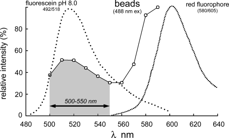
Fig. 1
Emission spectra of fluorescein with 492 nm excitation, the bead red fluorophore with 580 nm excitation, and beads containing both the red fluorophore and covalently attached fluorescein, with 488 nm ...
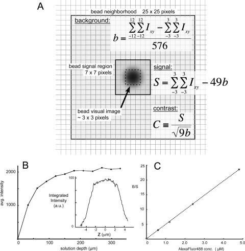
Fig. 2
(A) Diagram of the measurement regions described in the text. The diagram represents a portion of a digital image containing a single bead. Grey lines denote pixel boundaries. A grey-scale representat...
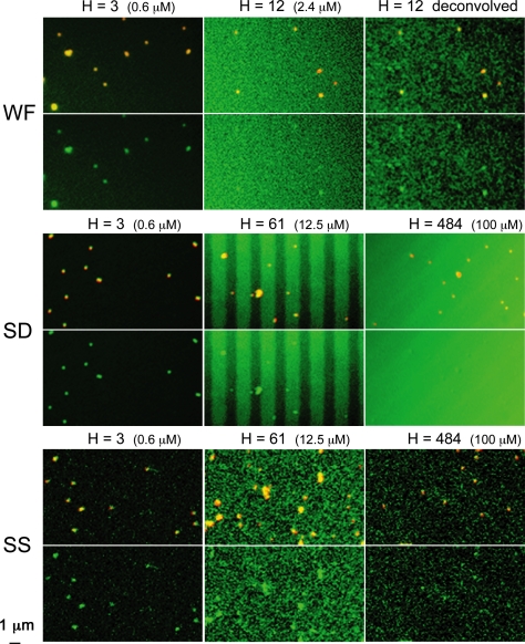
Fig. 3
Montage of images of beads with different amounts of out of focus fluorescence ( haziness index, H) from wide-field (WF), spinning disk (SD) and spot scanning (SS) confocal microscopes. The concentrat...
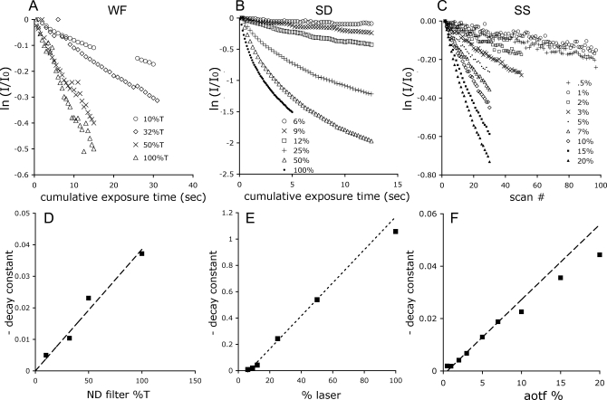
Fig. 4
Photobleaching curves used for calibration of the illumination systems. (A, B, C) Semilogarithmic plot of the normalized fluorescence intensity (ln( I / I 0 ) of the green fluorophore in a series of i...
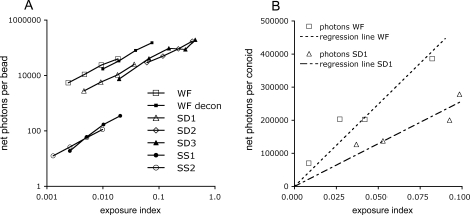
Fig. 5
(A) The average number of photons acquired from a single bead in images from WF, deconvolved WF (WFD), spinning disk confocal (SD) and spot scanning confocal microscopes (SS), plotted against standard...
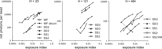
Fig. 6
Average net photons acquired from a single bead by microscopes of different types, plotted against standardized illumination dosage, for three different levels of out-of-focus background ( haziness in...
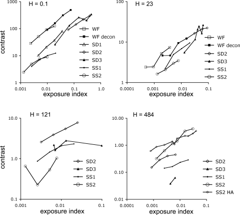
Fig. 7
Contrast in images of single beads acquired on different types of microscopes at 4 different levels of out-of-focus background ( haziness index , H) , plotted against standardized illumination dosage,...
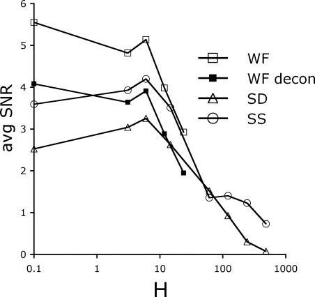
Fig. 8
Average SNR in populations of images of single beads acquired on different types of microscopes, plotted against the haziness index H (logarithmic scale for X -axis only). Data for all illumination do...
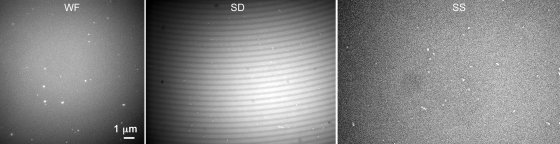
Fig. 9
Nonuniformity across the field of view in images from samples with high background acquired on ( left to right) WF, spinning disk confocal (SD) and spot scanning confocal (SS) microscopes. The bright ...
Figure images are served from the NIH/NLM PubMed Central Open Access Subset or Europe PMC; copyright remains with the publishers and authors.
💬 Discussion
0 commentsNo comments yet. Be the first to start a discussion!
Leave a Comment