Abstract
During mitosis, the connections of microtubules (MTs) to centrosomes and kinetochores are dynamic. From in vitro studies, it is known that the dynamic behavior of MTs is related to the structure of their ends, but we know little about the structure of MT ends in spindles. Here, we use high-voltage electron tomography to study the centrosome- and kinetochore-associated ends of spindle MTs in embryonic cells of the nematode, Caenorhabditis elegans. Centrosome-associated MT ends are either closed or open. Closed MT ends are more numerous and are uniformly distributed around the centrosome, but open ends are found preferentially on kinetochore-attached MTs. These results have structural implications for models of MT interactions with centrosomes.
🔬 Techniques
🧬 Organisms
💻 Software
🧪 Sample Preparation
🏭 Microscope Brands
🧪 Reagent Suppliers
📷 Detectors
💻 Software Details
💾 Data Repositories
🏛️ Research Organizations (ROR)
Affiliated research institutions:
📋 Methods
Specimen preparation for electron microscopy Wild-type C. elegans hermaphrodites were cryoimmobilized using a BAL-TEC HPM 010 high-pressure freezer (BAL-TEC). Fixation was performed by freeze substitution over 3 d at −90°C in anhydrous acetone containing 1% OsO 4 and 0.1% uranyl acetate (EM AFS; Leica) ( McDonald and Müller-Reichert, 2002 ). Epon/Araldite infiltrated samples were flat embedded in a thin layer of resin and polymerized for 3 d at 60°C ( Rappleye et al., 1999 ). Worms containing >5 early embryos were selected by light microscopy before remounting. Serial semithick sections (300–400 nm) were cut using a Leica Ultracut UCT Microtome. Sections were collected on Formvar-coated copper slot grids and poststained with 2% uranyl acetate in 70% methanol and Reynold's lead citrate.
High-voltage electron tomography
Electron tomography was performed essentially as described in O'Toole et al. (1999) . Briefly, 15-nm colloidal gold particles (Sigma-Aldrich) were attached to both surfaces of the semi-thick sections to serve as fiducial markers for subsequent image alignment. The specimens were placed in a tilt-rotate specimen holder (Model 650; Gatan, Pleasanton, CA) and tomographic datasets recorded using a JEM-1000 high-voltage electron microscope (JEOL, USA) operated at 750 kV. Images were captured every 1.5° over a ± 60° range using a Gatan 1K × 1K CCD camera at a pixel size of 1.4 nm. In some instances, montages of 2 × 1 or 3 × 1 frames were collected and used to image larger areas ( Marsh et al., 2001 ). For dual axis tomography, the grids were imaged in one tilt series then rotated 90°, and a similar tilt series was acquired. For image processing, images were transferred to a Silicon Graphics workstation, and the tilted views were aligned using the positions of the colloidal gold particles as fiducial points. Tomograms were computed for each tilt axis using the R-weighted back-projection algorithm ( Gilbert, 1972 ). We used the ratio of the section thickness, as defined by the microtome's setting, to the section's thickness measured after microscopy to calculate a “thinning factor,” which was then used to correct the tomogram's dimension along the beam axis ( O'Toole et al., 1999 ). For double tilt data sets, the two tomograms were aligned to each other and combined ( Mastronarde, 1997 ). In addition, tomograms computed from adjacent serial sections were aligned and joined to increase the reconstructed volume ( Ladinsky et al., 1999 ; Marsh et al., 2001 ). We recorded 11 double tilt series of mitotic spindles. In total, we analyzed 5 mitotic centrosomes.
Show full methods section
Specimen preparation for electron microscopy Wild-type C. elegans hermaphrodites were cryoimmobilized using a BAL-TEC HPM 010 high-pressure freezer (BAL-TEC). Fixation was performed by freeze substitution over 3 d at −90°C in anhydrous acetone containing 1% OsO 4 and 0.1% uranyl acetate (EM AFS; Leica) ( McDonald and Müller-Reichert, 2002 ). Epon/Araldite infiltrated samples were flat embedded in a thin layer of resin and polymerized for 3 d at 60°C ( Rappleye et al., 1999 ). Worms containing >5 early embryos were selected by light microscopy before remounting. Serial semithick sections (300–400 nm) were cut using a Leica Ultracut UCT Microtome. Sections were collected on Formvar-coated copper slot grids and poststained with 2% uranyl acetate in 70% methanol and Reynold's lead citrate.
High-voltage electron tomography
Electron tomography was performed essentially as described in O'Toole et al. (1999) . Briefly, 15-nm colloidal gold particles (Sigma-Aldrich) were attached to both surfaces of the semi-thick sections to serve as fiducial markers for subsequent image alignment. The specimens were placed in a tilt-rotate specimen holder (Model 650; Gatan, Pleasanton, CA) and tomographic datasets recorded using a JEM-1000 high-voltage electron microscope (JEOL, USA) operated at 750 kV. Images were captured every 1.5° over a ± 60° range using a Gatan 1K × 1K CCD camera at a pixel size of 1.4 nm. In some instances, montages of 2 × 1 or 3 × 1 frames were collected and used to image larger areas ( Marsh et al., 2001 ). For dual axis tomography, the grids were imaged in one tilt series then rotated 90°, and a similar tilt series was acquired. For image processing, images were transferred to a Silicon Graphics workstation, and the tilted views were aligned using the positions of the colloidal gold particles as fiducial points. Tomograms were computed for each tilt axis using the R-weighted back-projection algorithm ( Gilbert, 1972 ). We used the ratio of the section thickness, as defined by the microtome's setting, to the section's thickness measured after microscopy to calculate a “thinning factor,” which was then used to correct the tomogram's dimension along the beam axis ( O'Toole et al., 1999 ). For double tilt data sets, the two tomograms were aligned to each other and combined ( Mastronarde, 1997 ). In addition, tomograms computed from adjacent serial sections were aligned and joined to increase the reconstructed volume ( Ladinsky et al., 1999 ; Marsh et al., 2001 ). We recorded 11 double tilt series of mitotic spindles. In total, we analyzed 5 mitotic centrosomes.
Modeling and analysis of tomographic data
Tomograms were displayed and analyzed using the IMOD software package ( Kremer et al., 1996 ). Features of interest were modeled in the serial slices extracted from the tomogram. An “image slicer” window in IMOD was used to display a slice extracted from the 3-D volume in any position or orientation; this feature was useful for unambiguous tracking of MTs in 3-D ( O'Toole et al., 1999 ). With the slicer window, we analyzed the morphology of MT ends near the centrosomes and kinetochores by extracting a slice of image data 1-voxel thick and adjusting its orientation to contain the axis of the MT in a single view ( O'Toole et al., 1999 ). A projection of the 3-D model was displayed and rotated to study its 3-D geometry. For this display in 3-D, MTs were shown as tubular graphic objects. A program was written to compute the distance between the points on a selected object and a chosen reference location. The centroid of each centriole was located and used as the reference for positions within the spindle. A single model point was located at the pole-proximal end of each MT, and the 3-D distance of those points from the reference was calculated. A neighbor density analysis was performed to determine if there were preferred inter-fiber distances. These have been seen as indicative of interactions between different classes of MTs in two ( McDonald et al., 1992 ) and three dimensions ( Mastronarde et al., 1993 , Marsh et al., 2001 ). MT ends were classified as described ( Müller-Reichert et al., 1998 ). Online supplemental material Supplemental videos are available at http://www.jcb.org/cgi/content/full/jcb.200304035/DC1 . Videos 1 and 2 show the complete tomographic volume of centrosomes in metaphase and anaphase corresponding to Fig. 1, A and D , respectively. Videos 3 and 4 are the projected 3-D models corresponding to Fig. 1, B and C, and E and F , respectively. Video 5 corresponds to Fig. 3 A and shows the tomographic reconstruction of a kinetochore region in metaphase, and Video 6 shows the projected 3-D model displayed in Fig. 3 B. The video sequence associated with Fig. 4 B (Video 7) shows a movie through a tomographic reconstruction of a kinetochore region in greater detail. Video 8, corresponding to Fig. 5, A and B , illustrates the tracing of KMTs in a partially reconstructed metaphase spindle.
Online supplemental material Supplemental videos are available at http://www.jcb.org/cgi/content/full/jcb.200304035/DC1 . Videos 1 and 2 show the complete tomographic volume of centrosomes in metaphase and anaphase corresponding to Fig. 1, A and D , respectively. Videos 3 and 4 are the projected 3-D models corresponding to Fig. 1, B and C, and E and F , respectively. Video 5 corresponds to Fig. 3 A and shows the tomographic reconstruction of a kinetochore region in metaphase, and Video 6 shows the projected 3-D model displayed in Fig. 3 B. The video sequence associated with Fig. 4 B (Video 7) shows a movie through a tomographic reconstruction of a kinetochore region in greater detail. Video 8, corresponding to Fig. 5, A and B , illustrates the tracing of KMTs in a partially reconstructed metaphase spindle.
Supplemental Material [Supplemental Material Index]
📊 Figures
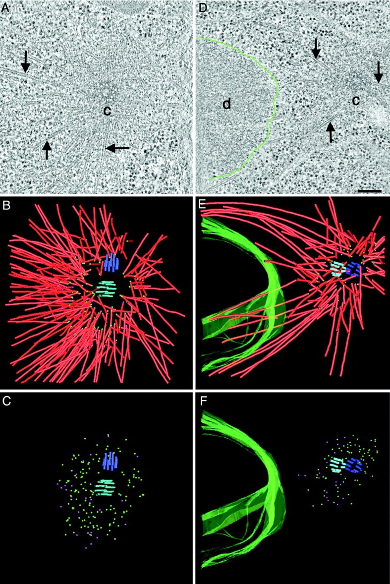
Figure 1.
MT ends at the centrosome are either closed or open. Distribution of MT minus ends around centrioles in metaphase (Au2013C) and anaphase (Du2013F). (A and D) Selected tomographic slices showing MTs (a...
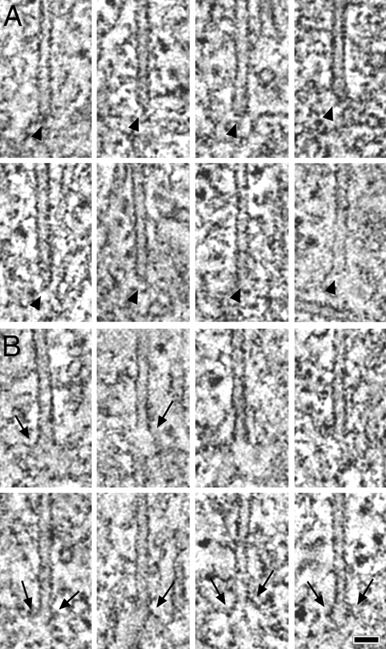
Figure 2.
Closed MT minus ends are pointed, open ends are blunt or slightly flared. (A) Capped minus ends. The ends of the MTs are marked by arrowheads. Capped MTs are often pointed and flattened on one side. (...
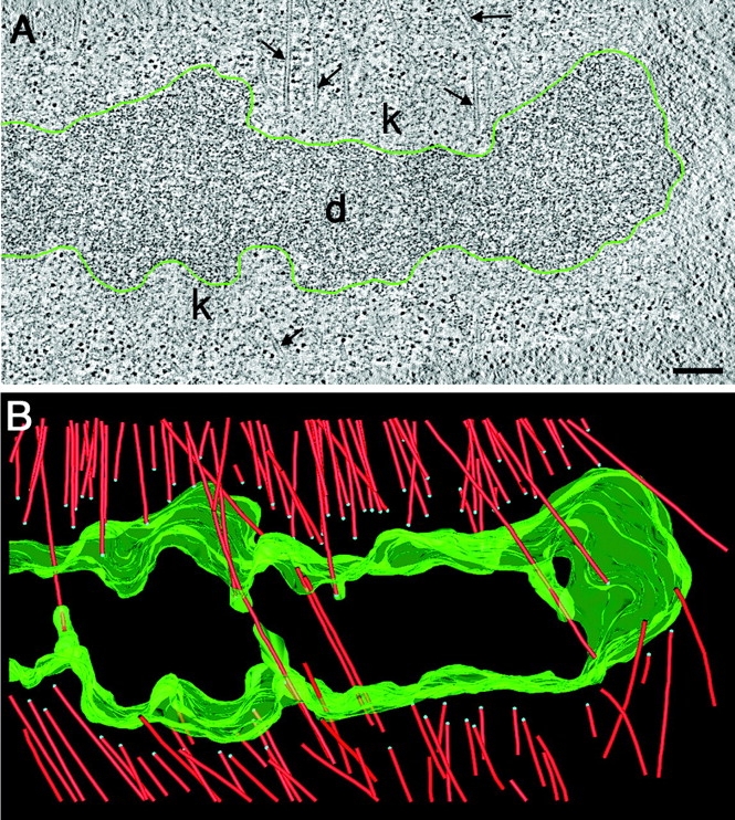
Figure 3.
KMTs do not end directly on the condensed chromatin. (A) Selected 2.7-nm thick tomographic slice showing a region at the metaphase plate. MTs (arrows) and the kinetochore regions (k) are indicated. Th...
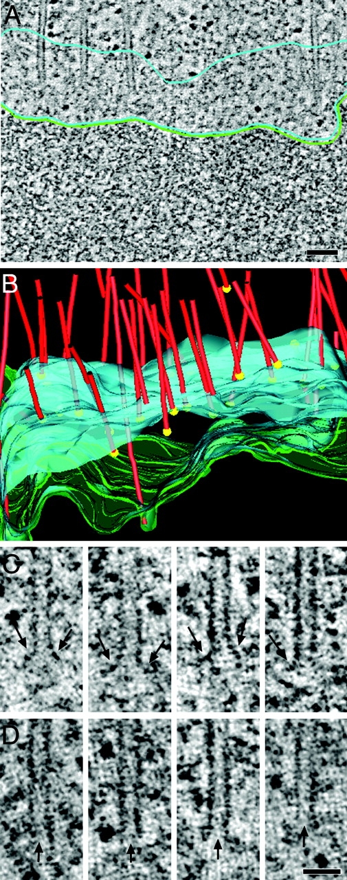
Figure 4.
KMT plus ends have an open, flared, or blunt morphology. (A) Detail of a kinetochore region as obtained by high-voltage electron tomography. KMTs terminate in the ribosome-free zone (outlined in light...
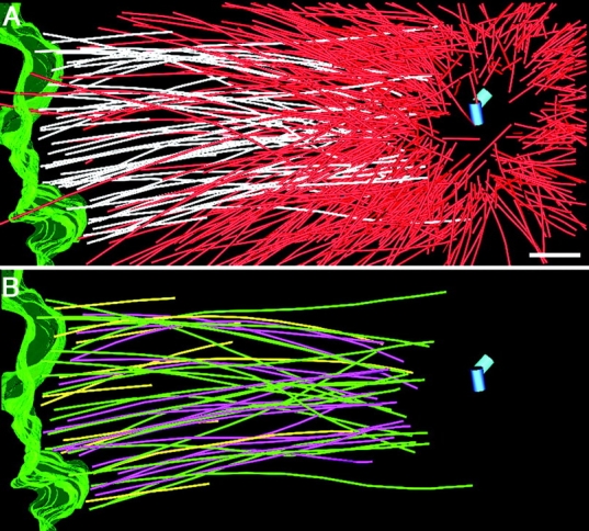
Figure 5.
Half of the KMT minus ends are open. (A) Partial reconstruction of a metaphase spindle. The surface of the DNA is outlined in green, and MTs that end in the ribosome-free zone are identified in white....
Figure images are served from the NIH/NLM PubMed Central Open Access Subset or Europe PMC; copyright remains with the publishers and authors.
💬 Discussion
0 commentsNo comments yet. Be the first to start a discussion!
Leave a Comment