Abstract
Human bone marrow mesenchymal stem cells (hBMSCs) are widely used cell source for clinical bone regeneration. Achieving the greatest therapeutic effect is dependent on the osteogenic differentiation potential of the stem cells to be implanted. However, there are still no practical methods to characterize such potential non-invasively or previously. Monitoring cellular morphology is a practical and non-invasive approach for evaluating osteogenic potential. Unfortunately, such image-based approaches had been historically qualitative and requiring experienced interpretation. By combining the non-invasive attributes of microscopy with the latest technology allowing higher throughput and quantitative imaging metrics, we studied the applicability of morphometric features to quantitatively predict cellular osteogenic potential. We applied computational machine learning, combining cell morphology features with their corresponding biochemical osteogenic assay results, to develop prediction model of osteogenic differentiation. Using a dataset of 9,990 images automatically acquired by BioStation CT during osteogenic differentiation culture of hBMSCs, 666 morphometric features were extracted as parameters. Two commonly used osteogenic markers, alkaline phosphatase (ALP) activity and calcium deposition were measured experimentally, and used as the true biological differentiation status to validate the prediction accuracy. Using time-course morphological features throughout differentiation culture, the prediction results highly correlated with the experimentally defined differentiation marker values (R>0.89 for both marker predictions). The clinical applicability of our morphology-based prediction was further examined with two scenarios: one using only historical cell images and the other using both historical images together with the patient's own cell images to predict a new patient's cellular potential. The prediction accuracy was found to be greatly enhanced by incorporation of patients' own cell features in the modeling, indicating the practical strategy for clinical usage. Consequently, our results provide strong evidence for the feasibility of using a quantitative time series of phase-contrast cellular morphology for non-invasive cell quality prediction in regenerative medicine.
🔬 Techniques
💻 Software
🧪 Sample Preparation
🔬 Cell Lines
🏭 Microscope Brands
🧪 Reagent Suppliers
💻 Software Details
🏛️ Research Organizations (ROR)
Affiliated research institutions:
📋 Methods
Cells and cell culture
Human bone-marrow derived mesenchymal stem cells (hBMSCs) (Lonza Walkersville, Inc., Maryland, U.S.A.) were subcultured (passaged) in Dulbecco's modified Eagles' medium (DMEM) containing 10% fetal bovine serum (FBS) (Life Technologies Japan Ltd., Tokyo, Japan). Three lots of hBMSCs were designated as Lot 1 (strain number 15000-1, unknown race, Male, 19-year-old), Lot 2 (strain number 17174, Oriental, Male, 20-year-old), and Lot 3 (strain number 11533, Black, Male, 22-year-old), respectively. Lot 1 and 2 were cultured to passages 3, 4, and 5, and Lot 3 was cultured to passages 6, 7, and 8, and cryopreserved for the start of the image acquisition experiment. Cryopreserved cells were seeded at a density of 1.0×10 4 cells/well in 12-well plate (Greiner Bio-One., Frickenhausen, Germany), and the cell-seeding day was designated as day 0 in the image acquisition experiment. Fig. 1 illustrates the experimental scheme for hBMSC osteogenic differentiation culture. From day 0 to 3, cells were cultured in 10% FBS-containing α-modified Eagle's medium (αMEM) (Sigma-Aldrich Co., St. Louis, MO, U.S.A.). From day 4 to 18, cells were divided into two groups: (1) Osteogenic induction group (Induction, N = 6) and (2) Non-induction group (Control, N = 6). For the induction group, the medium was switched to induction medium consisting of 10% FBS-containing αMEM medium supplemented with 10 nM dexamethasone (Sigma-Aldrich Co.), 100 mM ascorbic acid (Wako Pure Chemical Industries, Ltd., Osaka, Japan), and 10 mM glycerol 2-phosphate sodium salt hydrate (Sigma-Aldrich Co.). For the non-induction group, supplements were not added to the 10% FBS-containing αMEM medium. The appropriate medium was changed at day 7 and day 13. For half of the samples in each experimental group (n = 3), alkaline phosphatase (ALP) activity were quantified on day 18. The remaining samples continued culture until day 25, and calcium deposition was quantified on day 25. Image acquisition Figs. 1 and 10 -A illustrates the image acquisition scheme during hBMSC osteogenic differentiation culture. From day 0 to day 13 (14 days), phase contrast microscopic images of hBMSCs were obtained using the BioStation CT (Nikon Corporation, Tokyo, Japan). BioStation CT is an automatic cell maintenance system, which maintains a stable incubation environment (37°C, 5% CO 2, 100% humidity) with scheduled automatic image acquisition. The number of view fields was optimized to five, which provides the least error for estimating the correct cell seeding for each well. Five view fields (center position and four positions 2.2 mm from the center) of phase contrast images were acquired from each well with fully automatic focusing. The phase contrast images had the least noise and background when using the halo-reduction lens. Image acquisition timing was set to every 8 hours from day 4 to 18 (magnification = 10x). Time points are designated as time 0 to 38, indicating each of the 8 hour imaging intervals. Data at time 0 was omitted, since the cells were not fully settled. Data at time 7 and time 26 were also omitted, since it was concurrent with medium changes for each well plate, resulting in 36 time-points as a total. 10.1371/journal.pone.0055082.g010 Figure 10 A: Schematic illustration of cell image processing. The raw images were first pre-processed by background reduction processing by deconvolution and open-close filters. Then, images were binarized by the optimized threshold. The noisy objects were eliminated by particle deletion filter. B: Schematic illustration of cell morphology measurements and data processing. In all object recognized images, all existing objects were measured for the 9 morphological features. Since 1 condition was designed to consist of 3 wells ×5 view fields, all the corresponding object measurement results were processed as a same sample. The average and standard deviation within one sample of all morphological features at each time point were used as the input features for modeling. C: Schematic illustration of prediction model construction. Prediction of differentiation potential consisted of two steps. First, two types of prediction models (D14_ALP model or D21_Ca model) were constructed with the set of image data and experimental evaluation. Second, the values of D14_ALP or the D21_Ca were predicted from the input features of the sample targeted for prediction. The predicted biological rates are compared to the experimentally-determined results to evaluate the accuracy of prediction model.
Show full methods section
Cells and cell culture
Human bone-marrow derived mesenchymal stem cells (hBMSCs) (Lonza Walkersville, Inc., Maryland, U.S.A.) were subcultured (passaged) in Dulbecco's modified Eagles' medium (DMEM) containing 10% fetal bovine serum (FBS) (Life Technologies Japan Ltd., Tokyo, Japan). Three lots of hBMSCs were designated as Lot 1 (strain number 15000-1, unknown race, Male, 19-year-old), Lot 2 (strain number 17174, Oriental, Male, 20-year-old), and Lot 3 (strain number 11533, Black, Male, 22-year-old), respectively. Lot 1 and 2 were cultured to passages 3, 4, and 5, and Lot 3 was cultured to passages 6, 7, and 8, and cryopreserved for the start of the image acquisition experiment. Cryopreserved cells were seeded at a density of 1.0×10 4 cells/well in 12-well plate (Greiner Bio-One., Frickenhausen, Germany), and the cell-seeding day was designated as day 0 in the image acquisition experiment. Fig. 1 illustrates the experimental scheme for hBMSC osteogenic differentiation culture. From day 0 to 3, cells were cultured in 10% FBS-containing α-modified Eagle's medium (αMEM) (Sigma-Aldrich Co., St. Louis, MO, U.S.A.). From day 4 to 18, cells were divided into two groups: (1) Osteogenic induction group (Induction, N = 6) and (2) Non-induction group (Control, N = 6). For the induction group, the medium was switched to induction medium consisting of 10% FBS-containing αMEM medium supplemented with 10 nM dexamethasone (Sigma-Aldrich Co.), 100 mM ascorbic acid (Wako Pure Chemical Industries, Ltd., Osaka, Japan), and 10 mM glycerol 2-phosphate sodium salt hydrate (Sigma-Aldrich Co.). For the non-induction group, supplements were not added to the 10% FBS-containing αMEM medium. The appropriate medium was changed at day 7 and day 13. For half of the samples in each experimental group (n = 3), alkaline phosphatase (ALP) activity were quantified on day 18. The remaining samples continued culture until day 25, and calcium deposition was quantified on day 25. Image acquisition Figs. 1 and 10 -A illustrates the image acquisition scheme during hBMSC osteogenic differentiation culture. From day 0 to day 13 (14 days), phase contrast microscopic images of hBMSCs were obtained using the BioStation CT (Nikon Corporation, Tokyo, Japan). BioStation CT is an automatic cell maintenance system, which maintains a stable incubation environment (37°C, 5% CO 2, 100% humidity) with scheduled automatic image acquisition. The number of view fields was optimized to five, which provides the least error for estimating the correct cell seeding for each well. Five view fields (center position and four positions 2.2 mm from the center) of phase contrast images were acquired from each well with fully automatic focusing. The phase contrast images had the least noise and background when using the halo-reduction lens. Image acquisition timing was set to every 8 hours from day 4 to 18 (magnification = 10x). Time points are designated as time 0 to 38, indicating each of the 8 hour imaging intervals. Data at time 0 was omitted, since the cells were not fully settled. Data at time 7 and time 26 were also omitted, since it was concurrent with medium changes for each well plate, resulting in 36 time-points as a total. 10.1371/journal.pone.0055082.g010 Figure 10 A: Schematic illustration of cell image processing. The raw images were first pre-processed by background reduction processing by deconvolution and open-close filters. Then, images were binarized by the optimized threshold. The noisy objects were eliminated by particle deletion filter. B: Schematic illustration of cell morphology measurements and data processing. In all object recognized images, all existing objects were measured for the 9 morphological features. Since 1 condition was designed to consist of 3 wells ×5 view fields, all the corresponding object measurement results were processed as a same sample. The average and standard deviation within one sample of all morphological features at each time point were used as the input features for modeling. C: Schematic illustration of prediction model construction. Prediction of differentiation potential consisted of two steps. First, two types of prediction models (D14_ALP model or D21_Ca model) were constructed with the set of image data and experimental evaluation. Second, the values of D14_ALP or the D21_Ca were predicted from the input features of the sample targeted for prediction. The predicted biological rates are compared to the experimentally-determined results to evaluate the accuracy of prediction model.
Quantification of ALP activity Quantitative
ALP activity assays were performed as previously described [9] . After 18 days of culture, cell number was measured using a cell counting kit-8 (WST-8®; Dojindo Laboratories, Kumamoto, Japan), and ALP activities were measured with a p-nitrophenyl phosphate solution (Lab Assay ALP®; Wako Pure Chemical Industries, Ltd.). Briefly, for cell count, 100 µl of WST-8 was added to each well containing 1 mL of fresh medium, incubated for 1 hour, and absorbance was read at 450 nm. After WST-8 analysis, each well was washed twice with phosphate buffered saline (PBS) and 800 µL of p-nitrophenyl phosphate solution was added to each well. After 10 min of incubation at 37°C, the conversion to p-nitrophenol was stopped with 800 µl of 3N NaOH and the absorbance of p-nitrophenol was measured at 405 nm. Alkaline phosphatase-specific activity is expressed as p-nitrophenol absorbance (OD; 405 nm)/WST-8 absorbance (OD; 450 nm). Calcium deposition quantification After 25 days of culture, cells were fixed with 70% ethanol for 1 hour, washed, and stained for 10 min with 40 mM alizarin red S solution (pH: 4.2). After washing with PBS, plates were incubated with 10% cethylphridinium chloride for 15 min. Thereafter, supernatants were collected from each well and the absorption of each supernatant was measured at 405 nm to determine the amount of calcium deposition.
Cell image processing
All images (.bmp files) were processed by MetaMorph (Molecular device, CA, U.S.A) with the original combination of image-processing filter sets ( Fig. 10 –A). Briefly, the raw images were pre-processed by open-close filters and binarized by the optimized threshold. All image data was pre-processed using the same brightness threshold, which was optimized by 20 randomly picked image samples. This pre-processing step minimized error between the manually determined image cell number and the number of objects determined after pre-processing. After binarization, all individual objects in each image, consisting of cells and noise (non-cell objects), were measured by the integrated morphometric analysis function to measure morphological features (9 morphological features are: Breadth, Elliptical form factor, Fiber breadth, Fiber length, Hole area, Inner radius, Relative hole area, Shape factor, Total) ( Fig. 10 –B). The morphological features were carefully selected with the MetaMorph measurement function by logical selection. Features related to color and brightness were excluded first. Second, independent features were selected by hierarchical clustering and highly correlated features (R>0.85) were excluded. From the data consisting of object ID and its standardized 9 morphological features (average = 0, standard deviation = 1), the noise data (non-cell objects) was automatically cleansed by the original noise-reduction algorithm prior to the analysis (patent pending). From the pre-processed data, average (AVE) and standard deviation (SD) from each of the 9 morphological features was calculated from each of the cell objects covering five view fields from the same well, and used as the 18 inputs (9 features with AVE and SD) for each sample to be used in further analysis ( Fig. 10 –C). The morphological features and cell number (AVE and SD for 19th and 20th feature) from each well were then tagged with the target signals, which are experimentally determined values, resulting in 54 samples ( = 3 lots ×2 induction conditions ×3 passages ×3 wells) tagged with ALP values, and 54 samples tagged with calcium deposition values. This process links the “result” (biological measurement) with the “indication” (image-derived morphological feature), to derive a dataset for further modeling ( Fig. 10 –D).
Construction and evaluation of prediction model
Prediction of differentiation potential consists of two steps ( Fig. 10 –D): one is the construction of a prediction model, and the other is the evaluation of the constructed model. Using Ridge regression, two types of prediction models were constructed: (1) D14_ALP model, and (2) D21_Ca model. For the new patient scheme, prediction models were trained with 36 samples from 2 lots, and 18 samples from the remaining single lot were predicted. For the ongoing patient scheme, prediction models were trained with 42 samples from 2 lots of 3 passages plus the samples from new lot of 1 or 2 passages were used for training, and 12 samples from the remaining 1 lot were predicted ( Fig. 5 ). The detailed modeling process is described in a previous report (See Section 3 in [18] for details of the Ridge regression method). The performance of each of the models and datasets were evaluated by the average accuracy resulting from leave-one-out cross validation. For the evaluation of our proposed scheme, two evaluation indices are introduced in our work. One index is the correlation coefficient (R) of actual assay values and prediction values, which evaluates the prediction accuracy and its data coverage. The higher R increases, the more the model is capable of predicting “differentiation marker values” with small error rate. The other index of evaluation that we introduced is the average of absolute error. This value is calculated by obtaining absolute values of (experimentally determined value minus the predicted value). To compare these errors, we standardized these errors by dividing the variance of total experimentally determined values in one assay.
Supporting Information Table S1 * Exp. determined rate is the abbreviation of the experimentally determined rate. (XLS) Click here for additional data file. Table S2 * Exp. determined rate is the abbreviation of the experimentally determined rate. (XLSX) Click here for additional data file.
📊 Figures
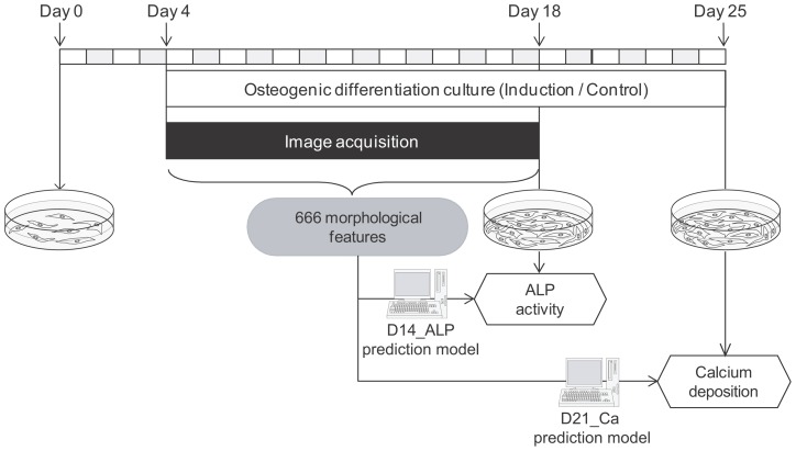
Figure 1
Schematic illustration of the experimental scheme for the prediction of osteogenic differentiation potential using multiple and time-course morphological features.
hBMSCs were cultured in non-induction medium in first 4 days, then the medium was replaced with osteogenic induction medium only for the Induction sample. From day 0 to day 14, cell images were automa...
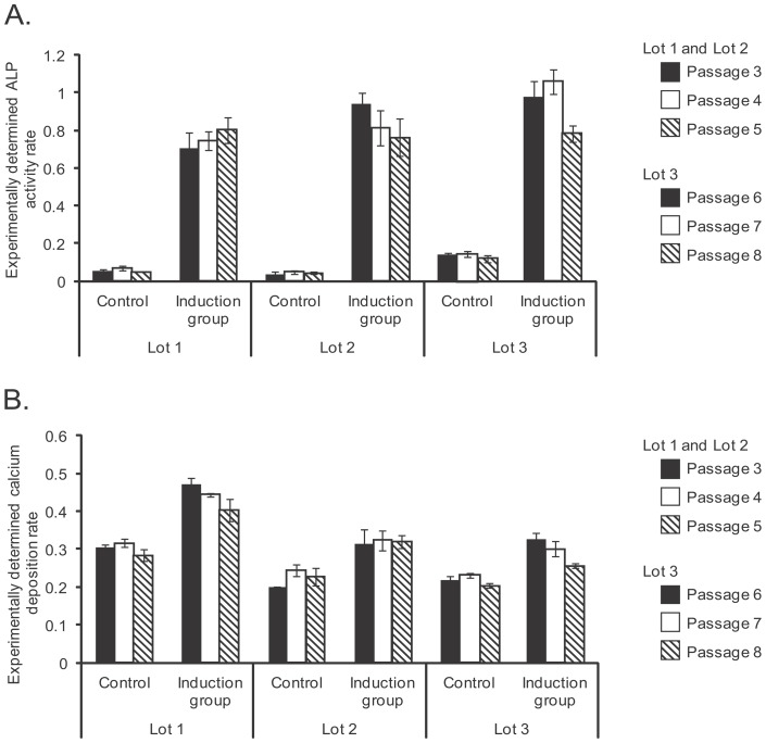
Figure 2
Experimentally determined biological results after the osteogenic differentiation.
A: Experimentally determined ALP activity rate on day 14 of differentiation. B: Experimentally determined calcium deposition rate on day 21 of differentiation.
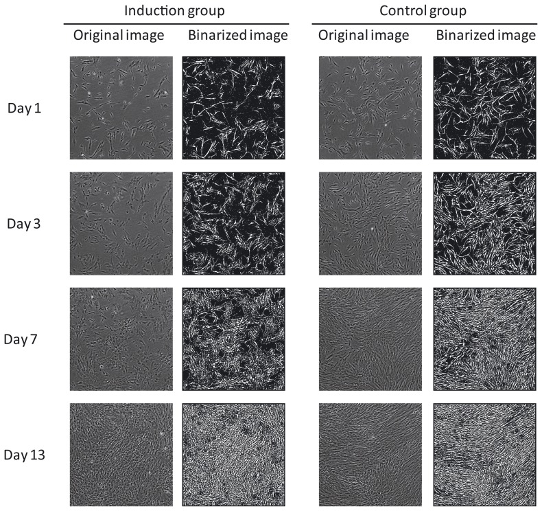
Figure 3
Phase contrast raw image from BioStation CT and its processed image.
The images of beginning (day 1), middle (day 3 and 7), and the end (day 13) in the induction period of Lot 1 are indicated as examples. Raw images were binarized with MetaMorph.
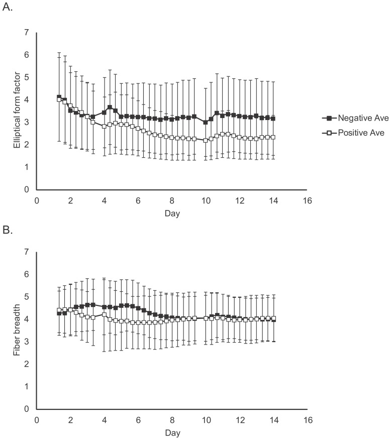
Figure 4
Time series changes of characteristic morphological features.
From the 9 morphological features measured, elliptical form factor (A) and fiber breadth (B) of Lot 1 are indicated as representative examples. The symbols indicate the mean value of each morphologica...
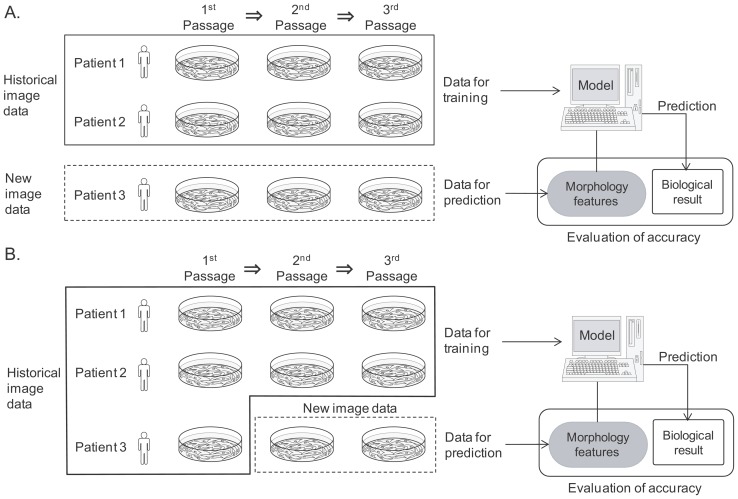
Figure 5
Schematic illustration of two scenarios examined to simulate clinical feasibility.
A: (Scenario I) New patient prediction scheme: Trained by historical patient dataset only. Images from all passages of patient 3 were used for prediction. B: (Scenario II) Ongoing patient prediction s...
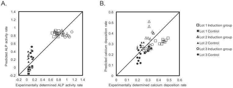
Figure 6
Prediction accuracies in the new patient scheme.
A: Scatter plot of experimentally determined values versus predicted values in D14_ALP model, B: Scatter plot of experimentally determined values versus predicted values in D21_Ca model.
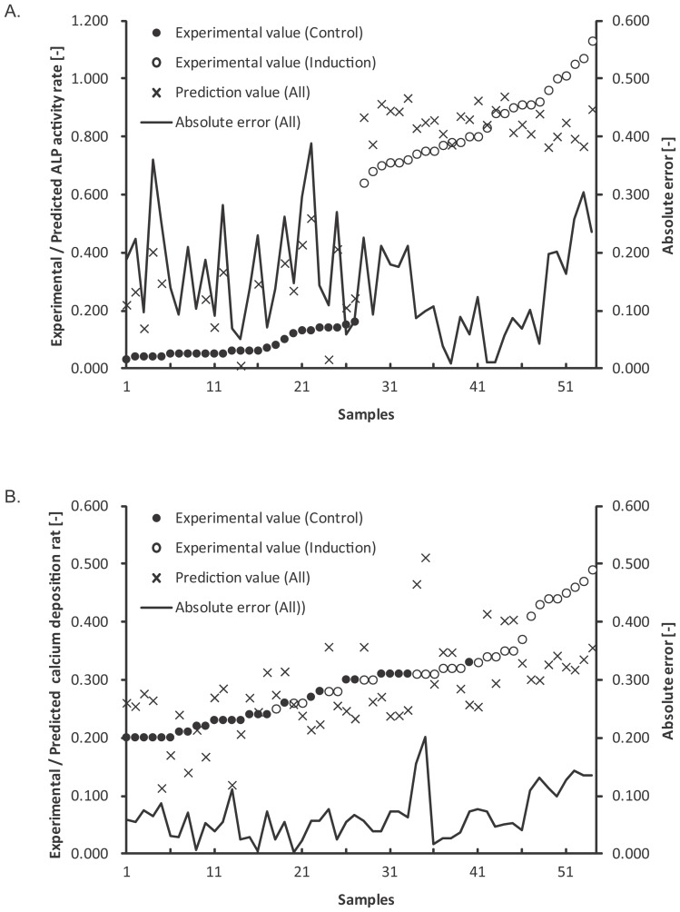
Figure 7
Detailed prediction results in new patient scheme.
A: Prediction results and error range in the D14_ALP model. B: Prediction results and error range in the D21_Ca model. All the plotted data were rearranged in the order of experimental values.
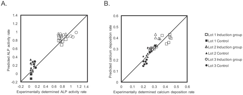
Figure 8
Prediction accuracies in the ongoing patient scheme.
A: Scatter plot of experimentally determined values versus predicted values in D14_ALP model, B: Scatter plot of experimentally determined values versus predicted values in D21_Ca model.
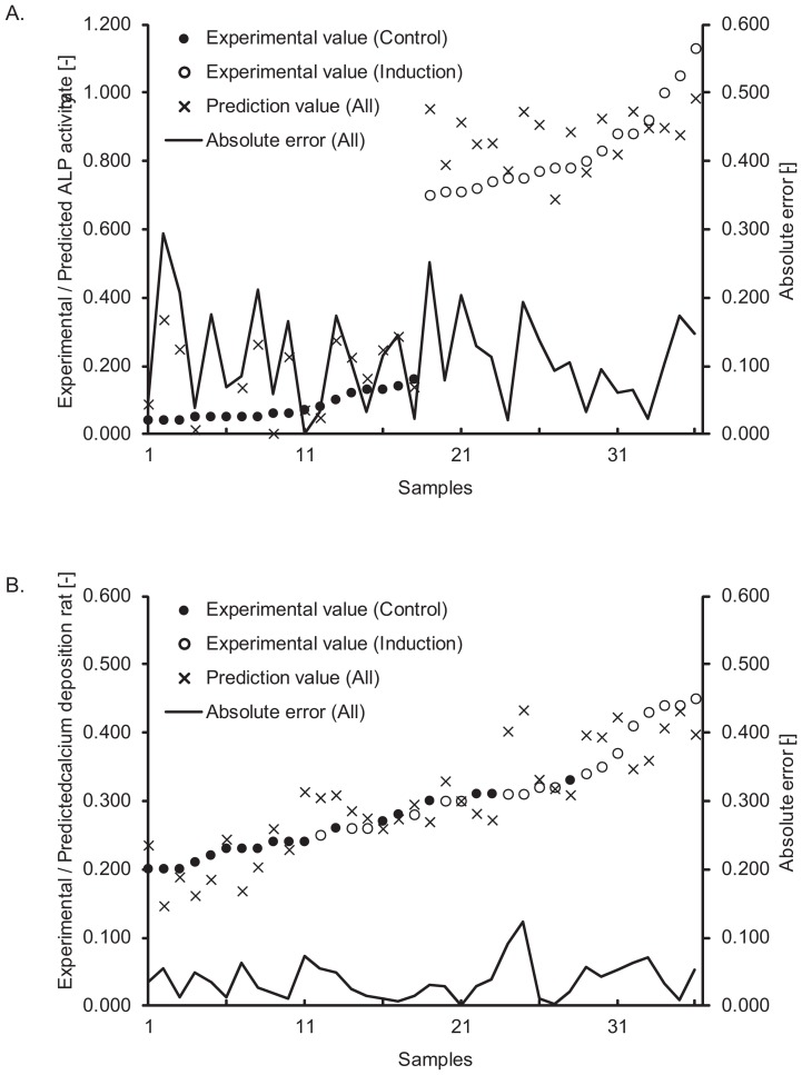
Figure 9
Detailed prediction results in ongoing patient scheme.
A: prediction results and error range in the D14_ALP model. B: Prediction results and error range in the D21_Ca model. All the plotted data were rearranged in the order of experimental values.
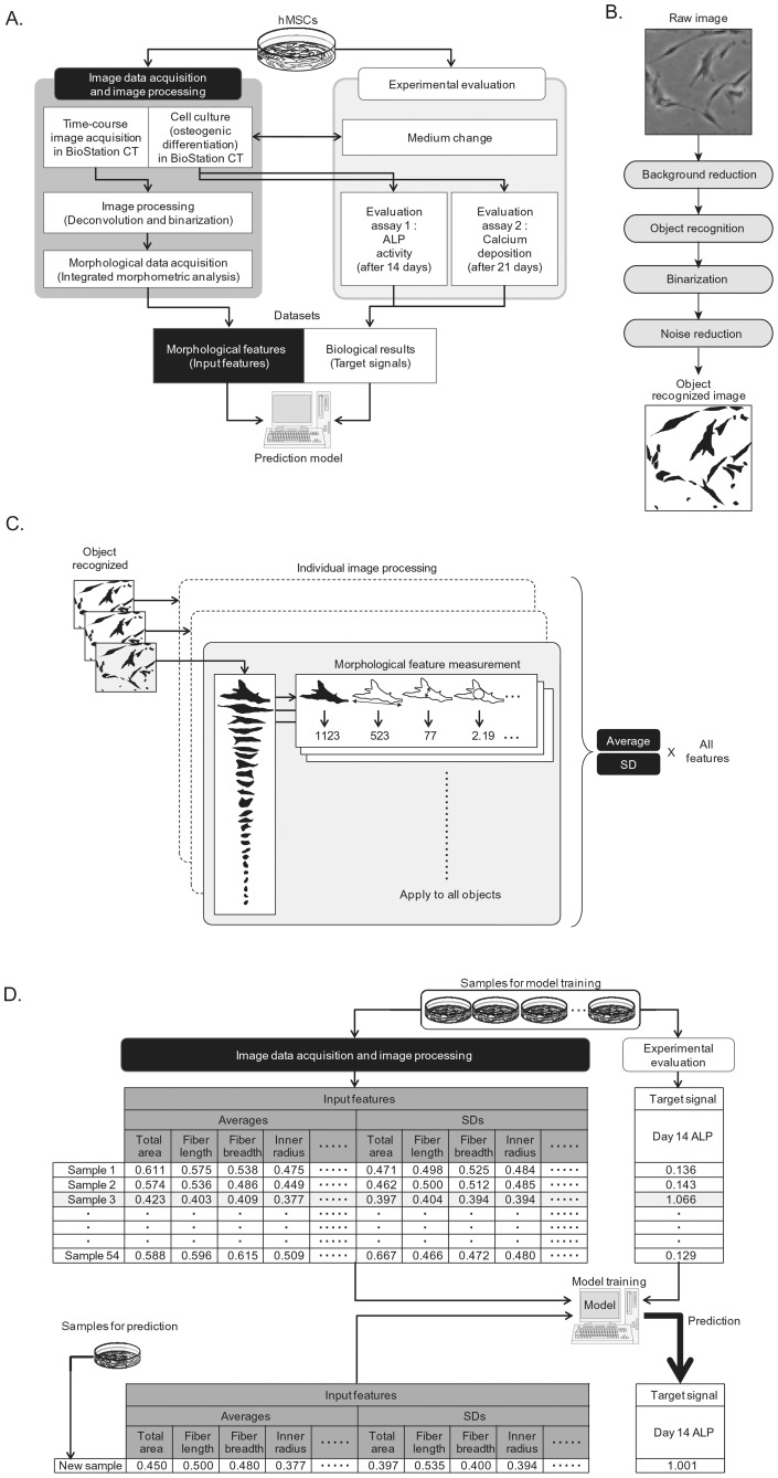
Figure 10
A: Schematic illustration of cell image processing.
The raw images were first pre-processed by background reduction processing by deconvolution and open-close filters. Then, images were binarized by the optimized threshold. The noisy objects were elimi...
Figure images are served from the NIH/NLM PubMed Central Open Access Subset or Europe PMC; copyright remains with the publishers and authors.
💬 Discussion
0 commentsNo comments yet. Be the first to start a discussion!
Leave a Comment