Abstract
During development, coordinated cell behaviors orchestrate tissue and organ morphogenesis. Detailed descriptions of cell lineages and behaviors provide a powerful framework to elucidate the mechanisms of morphogenesis. To study the cellular basis of limb development, we imaged transgenic fluorescently-labeled embryos from the crustacean Parhyale hawaiensis with multi-view light-sheet microscopy at high spatiotemporal resolution over several days of embryogenesis. The cell lineage of outgrowing thoracic limbs was reconstructed at single-cell resolution with new software called Massive Multi-view Tracker (MaMuT). In silico clonal analyses suggested that the early limb primordium becomes subdivided into anterior-posterior and dorsal-ventral compartments whose boundaries intersect at the distal tip of the growing limb. Limb-bud formation is associated with spatial modulation of cell proliferation, while limb elongation is also driven by preferential orientation of cell divisions along the proximal-distal growth axis. Cellular reconstructions were predictive of the expression patterns of limb development genes including the BMP morphogen Decapentaplegic.
🔬 Techniques
🔭 Microscopes
🧬 Organisms
💻 Software
✨ Fluorophores
🧪 Sample Preparation
🏭 Microscope Brands
🧪 Reagent Suppliers
🔎 Objectives
💻 Software Details
💻 Code & Software
💾 Data Repositories
🏛️ Research Organizations (ROR)
Affiliated research institutions:
📋 Methods
Key resources table
Reagent type (species) or resource Designation Source or reference Identifiers Additional information Strain, strain background ( Parhyale hawaiensis ) Wild Type PMID: 15986449 Strain, strain background ( P. hawaiensis ) PhHS>H2B-mRFPruby This paper Recombinant DNA reagent pMi{3xP3>EGFP; PhHS>H2B-mRFPruby} This paper Software, algorithm MaMuT This paper http://imagej.net/MaMuT Software, algorithm SIMI°BioCell PMID: 9133433 http://simi.com/en/products/cell-research Gene ( P. hawaiensis ) Ph-dpp This paper GenBank: KY696711 Gene ( P. hawaiensis ) Ph-Doc This paper GenBank: KY696712 Gene ( P. hawaiensis ) Ph-en2 This paper GenBank: KY696713 Gene ( P. hawaiensis ) Ph-H15 This paper Generation of transgenic Parhyale labeled with H2B-mRFPruby Parhyale hawaiensis ( Dana, 1853 ) rearing, embryo collection, microinjection and generation of transgenic lines were carried out as previously described ( Kontarakis and Pavlopoulos, 2014 ). To fluorescently label the chromatin in transgenic Parhyale , we fused the coding sequences of the Drosophila histone H2B and the mRFPruby monomeric Red Fluorescent Protein and placed them under control of a strong Parhyale heat-inducible promoter ( Pavlopoulos et al., 2009 ). H2B was amplified from genomic DNA with primers Dmel_H2B_F_NcoI (5’-TTAACCATGGCTCCGAAAACTAGTGGAAAG-3’) and Dmel_H2B_R_XhoI (5’-ACTTCTCGAGTTTAGAGCTGGTGTACTTGG-3’), and mRFPruby was amplified from plasmid pH2B-mRFPruby ( Fischer et al., 2006 ) with primers mRFPruby_F_XhoI (5’-ACAACTCGAGATGGGCAAGCTTACC-3’) and mRFPruby_R_PspMOI (5’-TATTGGGCCCTTAGGATCCAGCGCCTGTGC-3’). The NcoI/XhoI-digested H2B and XhoI/PspOMI-digested mRFPruby fragments were cloned in a triple-fragment ligation into NcoI/NotI-digested vector pSL-PhHS>DsRed, placing H2B-mRFPruby under control of the PhHS promoter ( Pavlopoulos et al., 2009 ). The PhHS>H2B-mRFPruby-SV40polyA cassette was then excised as an AscI fragment and cloned into the AscI-digested pMinos{3xP3>EGFP} vector ( Pavlopoulos and Averof, 2005 ; Pavlopoulos et al., 2004 ), generating plasmid pMi{3xP3>EGFP; PhHS>H2B-mRFPruby}. Three independent transgenic lines were established with this construct for heat-inducible expression of H2B-mRFPruby. The most strongly expressing line was selected for all applications. In this line, nuclear H2B-mRFPruby fluorescence plateaued about 12 hr after heat-shock and high levels of fluorescence persisted for at least 24 hr post heat-shock labeling chromatin in all cells throughout the cell cycle. Multi-view LSFM imaging of Parhyale embryos Standard procedures for multi-view LSFM recordings of Parhyale embryogenesis were established after imaging several dozen embryos individually in pilot experiments, first on a Zeiss prototype and, later on, on the commercial Zeiss Lightsheet Z.1 microscope. Several parameters described below were optimized to ensure that the two embryos used for lineage reconstruction (i) survived the recording process and hatched into juveniles without any morphological abnormalities, and (ii) were imaged with the appropriate spatiotemporal resolution and signal-to-noise ratio for accurate and comprehensive cell tracking in developing appendages. To prepare embryos for LSFM imaging, 2.5 day old transgenic embryos (early germband stage; S11 according to ( Browne et al., 2005 )) were heat-shocked for 1 hr at 37˚C. About 12 hr later (stage S13), they were mounted individually in a cylinder of 1% low melting agarose (SeaPlaque, Lonza) inside a glass capillary (#701902, Brand GmbH) with their AP axis aligned parallel to the capillary. A 1:4000 dilution of red fluorescent beads (#F-Y050 microspheres, Estapor Merck) were included in the agarose as fiducial markers for multi-view reconstruction. During imaging, the embedded embryo was extruded from the capillary into the chamber filled with artificial seawater supplemented with antibiotics and antimycotics (FASWA; ( Kontarakis and Pavlopoulos, 2014 )). The FASWA in the chamber was replaced every 12 hr after each heat shock (see below). The Zeiss Lightsheet Z.1 microscope was equipped with a 20x/1.0 Plan Apochromat immersion detection objective and two 10x/0.2 air illumination objectives producing two light-sheets 5.1 µm thick at the waist and 10.2 µm thick at the edges of a 488 µm x 488 µm field of view. We started imaging Parhyale embryogenesis from three angles/views (the ventral side and the two ventral-lateral sides 45˚ apart from ventral view) during 3 to 4.5 days AEL to avoid photo-damaging the dorsal thin extra-embryonic tissue, and continued imaging from five views (adding the two lateral sides 90˚ apart from ventral view) during 4.5 to 8 days AEL. A multi-view acquisition was made every 7.5 min at 26˚C. The H2B-mRFPruby fluorescence levels were replenished regularly every 12 hr by raising the temperature in the chamber from 26˚C to 37˚C and heat-shocking the embryo for 1 hr. Each view (z-stack) was composed of 250 16-bit frames with voxel size 0.254 µm x 0.254 µm x 1 µm. Each 1920x1920 pixel frame was acquired using two pivoting light-sheets to achieve a more homogeneous illumination and reduced image distortions caused by light scattering and absorption across the field of view. Each optical slice was acquired with a 561 nm laser and exposure time of 50 msec. With these conditions, Parhyale embryos, like the one bearing the T2 limb#1 analyzed in detail with MaMuT, were imaged routinely for a minimum of 4 days or even up to hatching. After hatching, the morphology of imaged specimen was compared between the left and the right side, as well as to its non-imaged siblings, to confirm that no obvious developmental or morphological abnormalities were detected. The embryo bearing the T2 limb#2 was imaged on a Zeiss LSFM prototype ( Preibisch et al., 2010 ) that offered single-sided illumination and single-sided detection with a 40x/0.8 immersion objective. One side of this embryo was imaged from 3 views 40˚ apart (ventral, ventral-left and left) every 7.5 min over a period of 66 hr. Each view was composed of 150 frames (1388 × 1080 pixels) with voxel size 0.366 µm x 0.366 µm x 2 µm. The embryo was imaged at 29–30˚C and was heat-shocked for 1 hr twice a day by perfusing warm FASWA at 37 ˚C. Cell tracking was carried out with the SIMI°BioCell software ( Hejnol and Scholtz, 2004 ; Schnabel et al., 1997 ) on a single view, the ventral-left view, of this dataset. Lineage reconstruction of limb#2 with SIMI°BioCell was complete up to about 22 hr of imaging time (35 hr when scaled to the growth rate of limb#1). After this time-point, an increasing number of cells in limb#2, in particular the descendant cells from the medial columns, became intractable. 4d reconstruction of Parhyale embryogenesis from multi-view LSFM image datasets Parhyale LSFM acquisitions typically resulted in 192 time-points/240K images/1.7 TB of raw data per day. Image processing was carried out on a MS Windows 7 Professional 64-bit workstation with 2 Intel Xeon E5-2687W processors, 256 GB RAM (16 X DIMMs 16384 MB 1600 MHz ECC DDR3), 4.8 TB hard disk space (2 × 480 GB and 6 × 960 GB Crucial M500 SATA 6 Gb/s SSD), 2 NVIDIA Quadro K4000 graphics cards (3 GB GDDR5). The workstation was connected through a 10 GB network interface to a MS Windows 2008 Server with 2 Intel Xeon E5-2680 processors, 196 GB RAM (24 X DIMM 8192 MB 1600 MHz ECC DDR3) and 144 TB hard disk space (36 X Seagate Constellation ES.3 4000 GB 7200 RPM 128 MB Cache SAS 6.0 Gb/s). All major LSFM image data processing steps were done with software modules available through the Multiview Reconstruction Fiji plugin ( http://imagej.net/Multiview-Reconstruction ) according to the following steps: Preprocessing: Image data acquired on Zeiss Lightsheet Z.1 were saved as an array of czi files labeled with ascending indices, where each file represented one view (z-stack). czi files were first renamed into the ‘spim_TL{t}_Angle{a}.czi’ filename, where t represented the time-point (e.g. 1 to 192 for a 1 day recording) and a the angle (e.g. 0 for left view, 45 for ventral-left view, 90 for ventral view, 135 for ventral-right view and 180 for right view), and then resaved as tif files. Bead-based spatial multi-view registration: In each time-point, all views were aligned to eachother and to an arbitrary reference view fixed in 3D space (e.g. views 0, 45, 90, 135 aligned to 180) using the bead-based registration option ( Preibisch et al., 2010 ). In each view, fluorescent beads scattered in the agarose were segmented with the Difference-of-Gaussian algorithm using a sigma value of 3 and an intensity threshold of 0.005. Corresponding beads were identified between views and were used to determine the affine transformation model that matched the views within each time-point. Fusion by multi-view deconvolution: Spatially registered views were down-sampled twice for time and memory efficient computations during the image fusion step. Input views were then fused into a single output 3D image with a more isotropic resolution using the Fiji plugin for multi-view deconvolution estimated from the point spread function of the fluorescent beads ( Preibisch et al., 2014 ). The same cropping area containing the entire imaged volume was selected for all time-points. In each time-point, the deconvolved fused image was calculated on GPU in blocks of 256 × 256×256 pixels with 7 iterations of the Efficient Bayesian method regularized with a Tikhonov parameter of 0.0006. Bead-based temporal registration: To correct for small drifts of the embryo over the extended imaging periods (e.g. due to agarose instabilities), we stabilized the fused volume over time using the segmented beads (sigma = 1.8 and intensity threshold = 0.005) for temporal registration with the affine transformation model using an all-to-all matching within a sliding window of 5 time-points. Computation of spatiotemporally registered fused volumes: Using the temporal registration parameters, we generated a stabilized time-series of the fused deconvolved 3D images. 4D rendering: The Parhyale embryo was rendered over time from the spatiotemporally registered fused data using Fiji’s 3D Viewer. Lineage reconstruction with the Massive Multi-view Tracker (MaMuT) MaMuT was developed as a tool for cell lineaging in multi-view LSFM image volumes by enabling to track objects synergistically from all available views. This functionality has a number of advantages. Raw views do not have to be fused into a single volume, which is computationally by far the most demanding step ( Preibisch et al., 2014 ). The users also preserve the original redundancy of the data, which in many cases like in Parhyale allows capturing cells from two or more neighboring views that can be interpreted independently for a more accurate analysis. Finally, MaMuT allows users to analyze sub-optimal datasets that cannot be fused properly or may create fusion artifacts. Of course, combining the raw views with a high-quality fused volume is the best available option, especially when handling complex datasets with high cell densities. While offering multi-view tracking, MaMuT delivers also other important functionalities. First, it is a turnkey software solution with a convenient interface for interactive exploration, annotation and curation of image data. Any image acquired by any microscopy modality that can be opened in Fiji can be also imported into MaMuT. Second, MaMuT offers a highly responsive and interactive navigation through multi-terabyte datasets. Individual z-stacks representing different views, channels and time-points of a multi-dimensional dataset can be displayed independently or in combinations in multiple synced Viewer windows. Third, objects of interest like cells and nuclei (spots) can be selected synergistically from all available Viewers and followed over time to reconstruct their trajectories (tracks) and lineage information. Fourth, the created spots and tracks can be visualized and edited interactively in the Viewers and the TrackScheme lineage browser, and animated in the 3D Viewer. For visual interpretation of the data, annotations can be colored based on the primary lineage information or derived numerical parameters. Fifth, lineages can be reconstructed in a manual, semi-automated or fully automated manner followed by manual curation if necessary. Sixth, all spot and track information can be exported from MaMuT to other interfaces for more specialized analyses. Seventh, decentralized annotation by multiple users has been made possible by also developing a web service for remote access to large image volumes stored online. Following on the tradition of the Fiji community for open-source distribution of biological image analysis software, MaMuT is provided freely and openly to the community, it is extensively documented and can be customized by other users. In practical terms, for lineaging purposes, the Parhyale multi-view LSFM raw views were registered spatiotemporally and the image data together with the registration parameters were converted into the custom HDF5/XML file formats utilized by the BigDataViewer and MaMuT Fiji plugins. The MaMuT reconstruction of the Parhyale T2 limb described in this article required about 10 weeks of dedicated manual cell tracking by an experienced annotator. The raw image data were displayed in Viewer windows and each z-stack was visualized in any desired color and brightness, scale (zoom), translation (position) and rotation (orientation). All Viewer windows were synced based on the calculated registration parameters and shared a common physical coordinate system; upon selecting an object of interest (spot) in one Viewer, the same spot was identified and displayed in all other windows, and its x, y, z position was mapped onto this common physical space. To guarantee the accuracy of our lineage reconstructions, the center of each tracked nucleus was verified in at least two neighboring views and by slicing the data orthogonally in separate Viewer windows. The nuclei contributing to the T2 limb of interest were identified in the first time-point and tracked manually every five time-points except during mitosis, in which case we also tracked one time-point before and one after segregation of the daughter chromosomes during anaphase/telophase. The reconstructed trajectories and lineages were also displayed in two additional synced windows, the TrackScheme and the 3D Viewer. The TrackScheme lineage browser and editor displayed the reconstructed cell lineage tree with tracked nuclei represented as nodes connected by edges over time and cell divisions depicted as split branches in the tree. The 3D Viewer window displayed interactive animations of the spots depicted as spheres and their tracks over time. The spots and the tracks in the Viewer, TrackScheme and 3D Viewer windows could be color-coded by lineage, position and other numerical features to assist visual analysis and interpretation of the data. In addition, all these windows were synced to simultaneously highlight active spots of interest at the selected time-point, greatly facilitating the cell lineaging process. Comparison of reconstructed lineage trees For comparative purposes, each reconstructed lineage tree was defined as a set of division times. For example, let’s consider a lineage tree L that starts with cell d. Cell d divides at time t 0 giving rise to the two daughter cells d 1 and d 2 . Then d 1 divides at time t 1 giving rise to daughter cells d 11 and d 12 . Finally, d 12 divides at time t 12 giving the daughter cells d 121 and d 122 . In this scenario, we define L as L = { t 0 , t 1 , t 12 } . Let’s now consider two lineage trees L x and L y , where x and y refer to the founder cells whose lineage trees are under comparison (e.g. x corresponds to E4c5 cell from limb#1 and y to E5b6 cell from limb#2). In order to be comparable, these two lineage trees need to be registered temporally. In our study, we performed a linear rescaling by an empirically determined factor of 1.6 to match the increase in cell number between limb#1 and limb#2 that were imaged at different temperatures and exhibited different growth rates. We then defined Δ ( L x , L y ) as the distance between the two registered lineage trees. This distance takes into consideration two metrics, the difference in the timing of divisions and the difference in the number of divisions between the two lineages, and is computed in the following way: Δ L x , L y = δ t L x , L y / n t + δ n ( L x , L y ) / n n 2 In this equation, δ t L x , L y is the difference in the timing of divisions and δ n ( L x , L y ) is the difference in the number of division between the two lineages. n t and n n are used to normalize the two metrics so that their values are comparable. They are defined as the maximum values observed for δ t L x , L y and δ n ( L x , L y ) in a given run of pairwise comparisons, i.e. they are the maximum values obtained in the 34 × 34 comparisons to calculate the distances between the 34 founder cells within limb#1 or within limb#2 or between limb#1 and limb#2. δ n is computed as the absolute value of the difference between the respective numbers of divisions in the two lineage trees: δ n L x , L y = C a r d ( L x - C a r d ( L y ) | To calculate δ t , we first paired the division times between the two lineage trees. For such a pairing P = { ( t i x , t j y ) | t i x ∈ L x , t j y ∈ L y } the difference in division times δ t ( P ) is computed as follows: δ t ( P ) = 1 C a r d ( P ) ∑ ( t i x , t j y ) ∈ P | t i x − t j y | The pairing P ⋆ that minimizes δ t is used to compute the temporal distance between the lineage trees. Let ℘ be the set of all possible pairings, then P ⋆ is defined as followed: P ⋆ = a r g m i n P ∈ P δ t ( P ) We then define δ t as δ t = δ t ( P ⋆ ) . Once we computed all the pairwise distances between lineages of the cells under comparison, hierarchical clustering was performed using Ward’s method. For the hierarchical clustering in the average Parhyale T2 limb, we combined for each founder cell the information from the two limbs. The average lineage tree L 12 x of lineage trees L 1 x = { t 11 x , t 12 x , t 13 x } and L 2 x = { t 21 x , t 22 x , t 23 x , t 24 x } , where x corresponds to the founder cell x with lineage trees L 1 x in limb#1 and L 2 x in limb#2, is defined as L 12 x = L 1 x ∪ L 2 x = { t 11 x , t 12 x , t 13 x , t 21 x , t 22 x , t 23 x , t 24 x } . The computation of the pairwise distance Δ between average lineage trees was then performed as described above.
Show full methods section
Key resources table
Reagent type (species) or resource Designation Source or reference Identifiers Additional information Strain, strain background ( Parhyale hawaiensis ) Wild Type PMID: 15986449 Strain, strain background ( P. hawaiensis ) PhHS>H2B-mRFPruby This paper Recombinant DNA reagent pMi{3xP3>EGFP; PhHS>H2B-mRFPruby} This paper Software, algorithm MaMuT This paper http://imagej.net/MaMuT Software, algorithm SIMI°BioCell PMID: 9133433 http://simi.com/en/products/cell-research Gene ( P. hawaiensis ) Ph-dpp This paper GenBank: KY696711 Gene ( P. hawaiensis ) Ph-Doc This paper GenBank: KY696712 Gene ( P. hawaiensis ) Ph-en2 This paper GenBank: KY696713 Gene ( P. hawaiensis ) Ph-H15 This paper Generation of transgenic Parhyale labeled with H2B-mRFPruby Parhyale hawaiensis ( Dana, 1853 ) rearing, embryo collection, microinjection and generation of transgenic lines were carried out as previously described ( Kontarakis and Pavlopoulos, 2014 ). To fluorescently label the chromatin in transgenic Parhyale , we fused the coding sequences of the Drosophila histone H2B and the mRFPruby monomeric Red Fluorescent Protein and placed them under control of a strong Parhyale heat-inducible promoter ( Pavlopoulos et al., 2009 ). H2B was amplified from genomic DNA with primers Dmel_H2B_F_NcoI (5’-TTAACCATGGCTCCGAAAACTAGTGGAAAG-3’) and Dmel_H2B_R_XhoI (5’-ACTTCTCGAGTTTAGAGCTGGTGTACTTGG-3’), and mRFPruby was amplified from plasmid pH2B-mRFPruby ( Fischer et al., 2006 ) with primers mRFPruby_F_XhoI (5’-ACAACTCGAGATGGGCAAGCTTACC-3’) and mRFPruby_R_PspMOI (5’-TATTGGGCCCTTAGGATCCAGCGCCTGTGC-3’). The NcoI/XhoI-digested H2B and XhoI/PspOMI-digested mRFPruby fragments were cloned in a triple-fragment ligation into NcoI/NotI-digested vector pSL-PhHS>DsRed, placing H2B-mRFPruby under control of the PhHS promoter ( Pavlopoulos et al., 2009 ). The PhHS>H2B-mRFPruby-SV40polyA cassette was then excised as an AscI fragment and cloned into the AscI-digested pMinos{3xP3>EGFP} vector ( Pavlopoulos and Averof, 2005 ; Pavlopoulos et al., 2004 ), generating plasmid pMi{3xP3>EGFP; PhHS>H2B-mRFPruby}. Three independent transgenic lines were established with this construct for heat-inducible expression of H2B-mRFPruby. The most strongly expressing line was selected for all applications. In this line, nuclear H2B-mRFPruby fluorescence plateaued about 12 hr after heat-shock and high levels of fluorescence persisted for at least 24 hr post heat-shock labeling chromatin in all cells throughout the cell cycle. Multi-view LSFM imaging of Parhyale embryos Standard procedures for multi-view LSFM recordings of Parhyale embryogenesis were established after imaging several dozen embryos individually in pilot experiments, first on a Zeiss prototype and, later on, on the commercial Zeiss Lightsheet Z.1 microscope. Several parameters described below were optimized to ensure that the two embryos used for lineage reconstruction (i) survived the recording process and hatched into juveniles without any morphological abnormalities, and (ii) were imaged with the appropriate spatiotemporal resolution and signal-to-noise ratio for accurate and comprehensive cell tracking in developing appendages. To prepare embryos for LSFM imaging, 2.5 day old transgenic embryos (early germband stage; S11 according to ( Browne et al., 2005 )) were heat-shocked for 1 hr at 37˚C. About 12 hr later (stage S13), they were mounted individually in a cylinder of 1% low melting agarose (SeaPlaque, Lonza) inside a glass capillary (#701902, Brand GmbH) with their AP axis aligned parallel to the capillary. A 1:4000 dilution of red fluorescent beads (#F-Y050 microspheres, Estapor Merck) were included in the agarose as fiducial markers for multi-view reconstruction. During imaging, the embedded embryo was extruded from the capillary into the chamber filled with artificial seawater supplemented with antibiotics and antimycotics (FASWA; ( Kontarakis and Pavlopoulos, 2014 )). The FASWA in the chamber was replaced every 12 hr after each heat shock (see below). The Zeiss Lightsheet Z.1 microscope was equipped with a 20x/1.0 Plan Apochromat immersion detection objective and two 10x/0.2 air illumination objectives producing two light-sheets 5.1 µm thick at the waist and 10.2 µm thick at the edges of a 488 µm x 488 µm field of view. We started imaging Parhyale embryogenesis from three angles/views (the ventral side and the two ventral-lateral sides 45˚ apart from ventral view) during 3 to 4.5 days AEL to avoid photo-damaging the dorsal thin extra-embryonic tissue, and continued imaging from five views (adding the two lateral sides 90˚ apart from ventral view) during 4.5 to 8 days AEL. A multi-view acquisition was made every 7.5 min at 26˚C. The H2B-mRFPruby fluorescence levels were replenished regularly every 12 hr by raising the temperature in the chamber from 26˚C to 37˚C and heat-shocking the embryo for 1 hr. Each view (z-stack) was composed of 250 16-bit frames with voxel size 0.254 µm x 0.254 µm x 1 µm. Each 1920x1920 pixel frame was acquired using two pivoting light-sheets to achieve a more homogeneous illumination and reduced image distortions caused by light scattering and absorption across the field of view. Each optical slice was acquired with a 561 nm laser and exposure time of 50 msec. With these conditions, Parhyale embryos, like the one bearing the T2 limb#1 analyzed in detail with MaMuT, were imaged routinely for a minimum of 4 days or even up to hatching. After hatching, the morphology of imaged specimen was compared between the left and the right side, as well as to its non-imaged siblings, to confirm that no obvious developmental or morphological abnormalities were detected. The embryo bearing the T2 limb#2 was imaged on a Zeiss LSFM prototype ( Preibisch et al., 2010 ) that offered single-sided illumination and single-sided detection with a 40x/0.8 immersion objective. One side of this embryo was imaged from 3 views 40˚ apart (ventral, ventral-left and left) every 7.5 min over a period of 66 hr. Each view was composed of 150 frames (1388 × 1080 pixels) with voxel size 0.366 µm x 0.366 µm x 2 µm. The embryo was imaged at 29–30˚C and was heat-shocked for 1 hr twice a day by perfusing warm FASWA at 37 ˚C. Cell tracking was carried out with the SIMI°BioCell software ( Hejnol and Scholtz, 2004 ; Schnabel et al., 1997 ) on a single view, the ventral-left view, of this dataset. Lineage reconstruction of limb#2 with SIMI°BioCell was complete up to about 22 hr of imaging time (35 hr when scaled to the growth rate of limb#1). After this time-point, an increasing number of cells in limb#2, in particular the descendant cells from the medial columns, became intractable. 4d reconstruction of Parhyale embryogenesis from multi-view LSFM image datasets Parhyale LSFM acquisitions typically resulted in 192 time-points/240K images/1.7 TB of raw data per day. Image processing was carried out on a MS Windows 7 Professional 64-bit workstation with 2 Intel Xeon E5-2687W processors, 256 GB RAM (16 X DIMMs 16384 MB 1600 MHz ECC DDR3), 4.8 TB hard disk space (2 × 480 GB and 6 × 960 GB Crucial M500 SATA 6 Gb/s SSD), 2 NVIDIA Quadro K4000 graphics cards (3 GB GDDR5). The workstation was connected through a 10 GB network interface to a MS Windows 2008 Server with 2 Intel Xeon E5-2680 processors, 196 GB RAM (24 X DIMM 8192 MB 1600 MHz ECC DDR3) and 144 TB hard disk space (36 X Seagate Constellation ES.3 4000 GB 7200 RPM 128 MB Cache SAS 6.0 Gb/s). All major LSFM image data processing steps were done with software modules available through the Multiview Reconstruction Fiji plugin ( http://imagej.net/Multiview-Reconstruction ) according to the following steps: Preprocessing: Image data acquired on Zeiss Lightsheet Z.1 were saved as an array of czi files labeled with ascending indices, where each file represented one view (z-stack). czi files were first renamed into the ‘spim_TL{t}_Angle{a}.czi’ filename, where t represented the time-point (e.g. 1 to 192 for a 1 day recording) and a the angle (e.g. 0 for left view, 45 for ventral-left view, 90 for ventral view, 135 for ventral-right view and 180 for right view), and then resaved as tif files. Bead-based spatial multi-view registration: In each time-point, all views were aligned to eachother and to an arbitrary reference view fixed in 3D space (e.g. views 0, 45, 90, 135 aligned to 180) using the bead-based registration option ( Preibisch et al., 2010 ). In each view, fluorescent beads scattered in the agarose were segmented with the Difference-of-Gaussian algorithm using a sigma value of 3 and an intensity threshold of 0.005. Corresponding beads were identified between views and were used to determine the affine transformation model that matched the views within each time-point. Fusion by multi-view deconvolution: Spatially registered views were down-sampled twice for time and memory efficient computations during the image fusion step. Input views were then fused into a single output 3D image with a more isotropic resolution using the Fiji plugin for multi-view deconvolution estimated from the point spread function of the fluorescent beads ( Preibisch et al., 2014 ). The same cropping area containing the entire imaged volume was selected for all time-points. In each time-point, the deconvolved fused image was calculated on GPU in blocks of 256 × 256×256 pixels with 7 iterations of the Efficient Bayesian method regularized with a Tikhonov parameter of 0.0006. Bead-based temporal registration: To correct for small drifts of the embryo over the extended imaging periods (e.g. due to agarose instabilities), we stabilized the fused volume over time using the segmented beads (sigma = 1.8 and intensity threshold = 0.005) for temporal registration with the affine transformation model using an all-to-all matching within a sliding window of 5 time-points. Computation of spatiotemporally registered fused volumes: Using the temporal registration parameters, we generated a stabilized time-series of the fused deconvolved 3D images. 4D rendering: The Parhyale embryo was rendered over time from the spatiotemporally registered fused data using Fiji’s 3D Viewer. Lineage reconstruction with the Massive Multi-view Tracker (MaMuT) MaMuT was developed as a tool for cell lineaging in multi-view LSFM image volumes by enabling to track objects synergistically from all available views. This functionality has a number of advantages. Raw views do not have to be fused into a single volume, which is computationally by far the most demanding step ( Preibisch et al., 2014 ). The users also preserve the original redundancy of the data, which in many cases like in Parhyale allows capturing cells from two or more neighboring views that can be interpreted independently for a more accurate analysis. Finally, MaMuT allows users to analyze sub-optimal datasets that cannot be fused properly or may create fusion artifacts. Of course, combining the raw views with a high-quality fused volume is the best available option, especially when handling complex datasets with high cell densities. While offering multi-view tracking, MaMuT delivers also other important functionalities. First, it is a turnkey software solution with a convenient interface for interactive exploration, annotation and curation of image data. Any image acquired by any microscopy modality that can be opened in Fiji can be also imported into MaMuT. Second, MaMuT offers a highly responsive and interactive navigation through multi-terabyte datasets. Individual z-stacks representing different views, channels and time-points of a multi-dimensional dataset can be displayed independently or in combinations in multiple synced Viewer windows. Third, objects of interest like cells and nuclei (spots) can be selected synergistically from all available Viewers and followed over time to reconstruct their trajectories (tracks) and lineage information. Fourth, the created spots and tracks can be visualized and edited interactively in the Viewers and the TrackScheme lineage browser, and animated in the 3D Viewer. For visual interpretation of the data, annotations can be colored based on the primary lineage information or derived numerical parameters. Fifth, lineages can be reconstructed in a manual, semi-automated or fully automated manner followed by manual curation if necessary. Sixth, all spot and track information can be exported from MaMuT to other interfaces for more specialized analyses. Seventh, decentralized annotation by multiple users has been made possible by also developing a web service for remote access to large image volumes stored online. Following on the tradition of the Fiji community for open-source distribution of biological image analysis software, MaMuT is provided freely and openly to the community, it is extensively documented and can be customized by other users. In practical terms, for lineaging purposes, the Parhyale multi-view LSFM raw views were registered spatiotemporally and the image data together with the registration parameters were converted into the custom HDF5/XML file formats utilized by the BigDataViewer and MaMuT Fiji plugins. The MaMuT reconstruction of the Parhyale T2 limb described in this article required about 10 weeks of dedicated manual cell tracking by an experienced annotator. The raw image data were displayed in Viewer windows and each z-stack was visualized in any desired color and brightness, scale (zoom), translation (position) and rotation (orientation). All Viewer windows were synced based on the calculated registration parameters and shared a common physical coordinate system; upon selecting an object of interest (spot) in one Viewer, the same spot was identified and displayed in all other windows, and its x, y, z position was mapped onto this common physical space. To guarantee the accuracy of our lineage reconstructions, the center of each tracked nucleus was verified in at least two neighboring views and by slicing the data orthogonally in separate Viewer windows. The nuclei contributing to the T2 limb of interest were identified in the first time-point and tracked manually every five time-points except during mitosis, in which case we also tracked one time-point before and one after segregation of the daughter chromosomes during anaphase/telophase. The reconstructed trajectories and lineages were also displayed in two additional synced windows, the TrackScheme and the 3D Viewer. The TrackScheme lineage browser and editor displayed the reconstructed cell lineage tree with tracked nuclei represented as nodes connected by edges over time and cell divisions depicted as split branches in the tree. The 3D Viewer window displayed interactive animations of the spots depicted as spheres and their tracks over time. The spots and the tracks in the Viewer, TrackScheme and 3D Viewer windows could be color-coded by lineage, position and other numerical features to assist visual analysis and interpretation of the data. In addition, all these windows were synced to simultaneously highlight active spots of interest at the selected time-point, greatly facilitating the cell lineaging process. Comparison of reconstructed lineage trees For comparative purposes, each reconstructed lineage tree was defined as a set of division times. For example, let’s consider a lineage tree L that starts with cell d. Cell d divides at time t 0 giving rise to the two daughter cells d 1 and d 2 . Then d 1 divides at time t 1 giving rise to daughter cells d 11 and d 12 . Finally, d 12 divides at time t 12 giving the daughter cells d 121 and d 122 . In this scenario, we define L as L = { t 0 , t 1 , t 12 } . Let’s now consider two lineage trees L x and L y , where x and y refer to the founder cells whose lineage trees are under comparison (e.g. x corresponds to E4c5 cell from limb#1 and y to E5b6 cell from limb#2). In order to be comparable, these two lineage trees need to be registered temporally. In our study, we performed a linear rescaling by an empirically determined factor of 1.6 to match the increase in cell number between limb#1 and limb#2 that were imaged at different temperatures and exhibited different growth rates. We then defined Δ ( L x , L y ) as the distance between the two registered lineage trees. This distance takes into consideration two metrics, the difference in the timing of divisions and the difference in the number of divisions between the two lineages, and is computed in the following way: Δ L x , L y = δ t L x , L y / n t + δ n ( L x , L y ) / n n 2 In this equation, δ t L x , L y is the difference in the timing of divisions and δ n ( L x , L y ) is the difference in the number of division between the two lineages. n t and n n are used to normalize the two metrics so that their values are comparable. They are defined as the maximum values observed for δ t L x , L y and δ n ( L x , L y ) in a given run of pairwise comparisons, i.e. they are the maximum values obtained in the 34 × 34 comparisons to calculate the distances between the 34 founder cells within limb#1 or within limb#2 or between limb#1 and limb#2. δ n is computed as the absolute value of the difference between the respective numbers of divisions in the two lineage trees: δ n L x , L y = C a r d ( L x - C a r d ( L y ) | To calculate δ t , we first paired the division times between the two lineage trees. For such a pairing P = { ( t i x , t j y ) | t i x ∈ L x , t j y ∈ L y } the difference in division times δ t ( P ) is computed as follows: δ t ( P ) = 1 C a r d ( P ) ∑ ( t i x , t j y ) ∈ P | t i x − t j y | The pairing P ⋆ that minimizes δ t is used to compute the temporal distance between the lineage trees. Let ℘ be the set of all possible pairings, then P ⋆ is defined as followed: P ⋆ = a r g m i n P ∈ P δ t ( P ) We then define δ t as δ t = δ t ( P ⋆ ) . Once we computed all the pairwise distances between lineages of the cells under comparison, hierarchical clustering was performed using Ward’s method. For the hierarchical clustering in the average Parhyale T2 limb, we combined for each founder cell the information from the two limbs. The average lineage tree L 12 x of lineage trees L 1 x = { t 11 x , t 12 x , t 13 x } and L 2 x = { t 21 x , t 22 x , t 23 x , t 24 x } , where x corresponds to the founder cell x with lineage trees L 1 x in limb#1 and L 2 x in limb#2, is defined as L 12 x = L 1 x ∪ L 2 x = { t 11 x , t 12 x , t 13 x , t 21 x , t 22 x , t 23 x , t 24 x } . The computation of the pairwise distance Δ between average lineage trees was then performed as described above.
Analysis of gene expression
Parhyale decapentaplegic ( Ph-dpp ), Dorsocross ( Ph-Doc ), engrailed-2 ( Ph-en2 ) and H15 ( Ph-H15 ) genes were identified by BLAST analysis against the Parhyale transcriptome and genome ( Kao et al., 2016 ) using the protein sequence of Drosophila orthologs as queries. Sequence accession numbers are KY696711 for Ph-dpp , KY696712 for Ph-Doc , and KY696713 for Ph-en2 . Phylogenetic tree construction was performed with RAxML using the WAG + G model from MAFFT multiple sequence alignments trimmed with trimAl ( Stamatakis, 2014 ). In situ hybridizations were carried out as previously described ( Rehm et al., 2009 ). Stained samples were imaged on a Zeiss 880 confocal microscope using the Plan-Apochromat 10x/0.45 and 20x/0.8 objectives. Images were processed using Fiji and Photoshop CS6 (Adobe Systems Inc). For color overlays, the brightfield image of the Ph-dpp , Ph-Doc or Ph-H15 BCIP/NBT staining was inverted, false-colored green and merged with the fluorescent signal of the Ph-en2 FastRed staining in magenta and the nuclear DAPI signal in blue. In order to map gene expression patterns onto cell lineages, the z-stacks from imaged fixed specimens were imported into MaMuT and the manually reconstructed nuclei and annotated gene expression patterns were compared with the corresponding stages of the live imaged and lineaged embryos. This analysis was performed with single-cell accuracy thanks to the well characterized and invariant patterns of cell division across Parhyale embryos, the orderly arrangement of cells in the earlier stages analyzed, and the easily identifiable straight boundary between anterior and posterior cells in the later stages analyzed.
Additional files 10.7554/eLife.34410.026 Transparent reporting form Major datasets The following previously published dataset was used: Kao D Lai AG Stamataki E Rosic S Konstantinides N Jarvis E Di Donfrancesco A Pouchkina-Stancheva N Sémon M Grillo M Bruce H Kumar S Siwanowicz I Le A Lemire A Eisen MB Extavour C Browne WE Wolff C Averof M Patel NH Sarkies P Pavlopoulos A Aboobaker A 2016 Parhyale hawaiensis isolate:Chicago-F Genome sequencing and assembly https://www.ncbi.nlm.nih.gov/bioproject/306836 Publicly available at NCBI BioProject (accession no. PRJNA306836)
📊 Figures
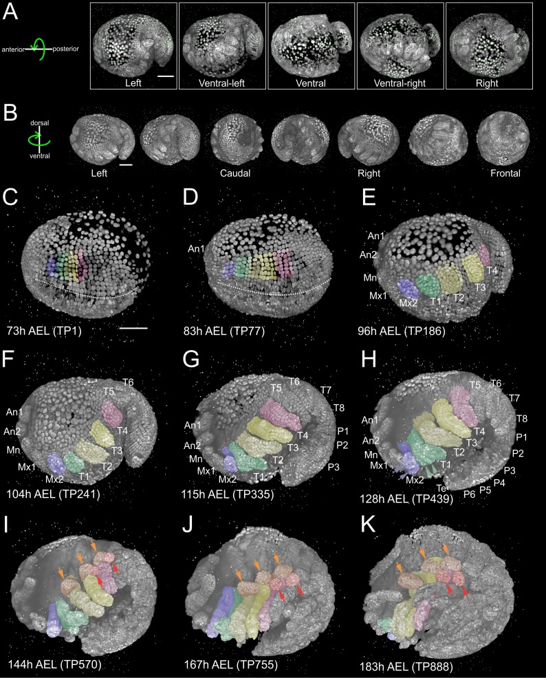
Figure 1.
Reconstruction of Parhyale embryogenesis with multi-view LSFM (see also Figure 1u2014video 1 and 2 ).
( A ) Transgenic Parhyale embryo with H2B-mRFPruby-labeled nuclei mounted with fluorescent beads (green dots) for multi-view reconstruction. The embryo was imaged from the indicated 5 views with 45u02...
Figure 1u2014video 1.
Imaging Parhyale embryogenesis with multi-view LSFM
Time-lapse recording of a transgenic embryo from the crustacean amphipod Parhyale hawaiensis labeled with the nuclear H2B-mRFPruby fluorescent marker. The embryo was recorded on a Zeiss Lightsheet Z.1...
Figure 1u2014video 2.
Imaging Parhyale embryogenesis with multi-view LSFM
Left side of the same embryo shown in Figure 1u2014video 1 rendered with the same settings but without rotation. Anterior is to the left and dorsal to the top.
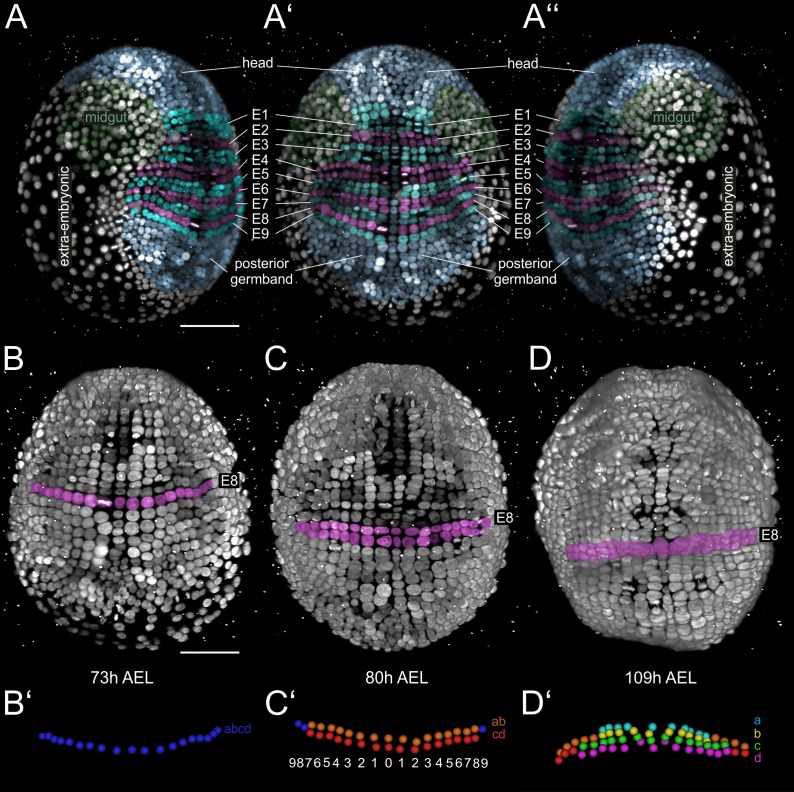
Figure 2.
Grid architecture of the Parhyale germband.
( Au2013Au2019u2019 ) Rendering of a Parhyale embryo at the growing germband stage: ( A ) Right, ( Au2019 ) ventral, and ( Au2019u2019 ) left side. Color masks indicate the anterior head region (blue)...
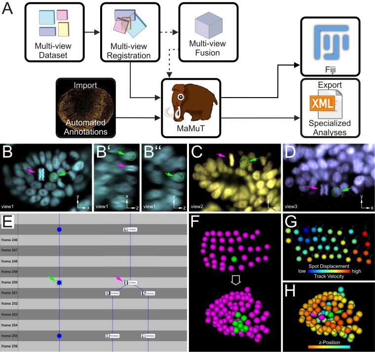
Figure 3.
Cell tracking and lineage reconstruction with MaMuT (see also Figure 3u2014figure supplement 1 ).
( A ) Workflow for image data analysis with MaMuT. Raw views (colored boxes in Multi-view Dataset) are registered (overlapping boxes in Multi-view Registration) and, optionally, fused into a single vo...
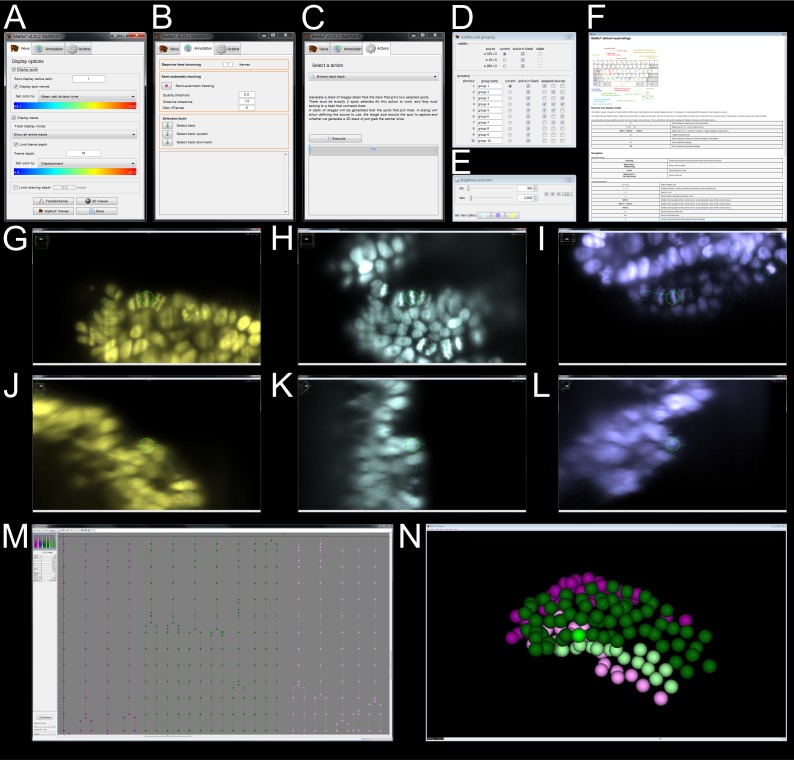
Figure 3u2014figure supplement 1.
MaMuT layout.
( Au2013C ) The three tabs of the MaMuT control panel. ( A ) The Views tab is used to launch and control the different displays of the image data and annotations. ( B ) The Annotation tab is used to d...
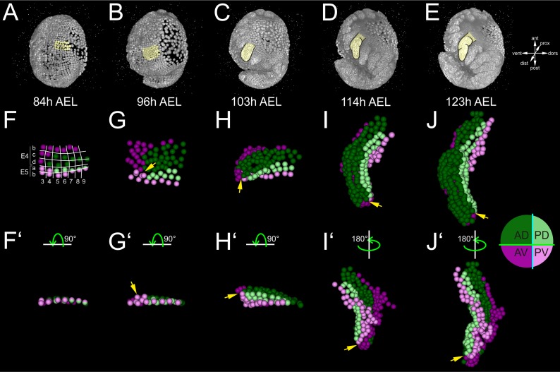
Figure 4.
Early compartmentalization of the Parhyale thoracic limb (see also Figure 4u2014figure supplements 1 and 2 ).
( Au2013E ) Lateral views of a Parhyale embryo rendered at the indicated developmental stages shown in hours (h) after egg-lay (AEL). Yellow masks show the left T2 limb (limb#1). ( Fu2013Ju2019 ) Trac...
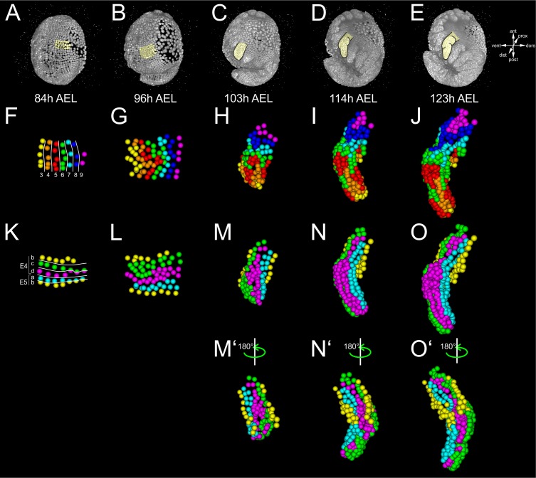
Figure 4u2014figure supplement 1.
Lineage reconstruction of the Parhyale thoracic limb.
( Au2013E ) Lateral views of the same Parhyale embryo shown in Figure 4 . Yellow masks indicate the left T2 limb (limb#1). ( Fu2013J ) Tracked cells contributing to the T2 limb color-coded by the DV c...
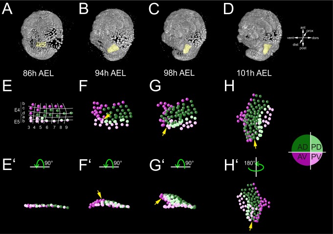
Figure 4u2014figure supplement 2.
Independent evidence for early compartmentalization of the Parhyale thoracic limb.
( Au2013D ) Lateral views of another Parhyale embryo imaged on a Zeiss LSFM prototype instrument rendered at the indicated developmental stages shown in hours (h) after egg-lay (AEL). Yellow masks ind...
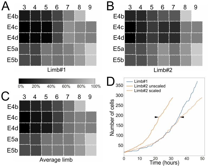
Figure 5.
Stereotyped and variable cell behaviors in developing Parhyale thoracic limbs (see also Figure 5u2014figure supplement 1 , Figure 5u2014source data 1 , and Figure 5u2014video 1 ).
( Au2013C ) Schematic representations of the T2 limb primordium at the 4-row-parasegment stage displaying the 34 founder cells as squares color-coded based on their relative birth times: ( A ) limb#1,...
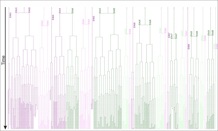
Figure 5u2014figure supplement 1.
Reconstructed lineage tree of a Parhyale T2 limb.
Each track resembles one or two of the 34 founder cells of limb#1 color-coded by their compartmental identity: anterior-dorsal in dark green, anterior-ventral in dark magenta, posterior-dorsal in ligh...
Figure 5u2014video 1.
Animation of tracked cells forming the Parhyale second thoracic limb
All tracked cells contributing to the T2 limb#1 are displayed as spheres of uniform color. The movie starts from the early limb specification stage at about 3 days AEL and covers limb bud formation an...
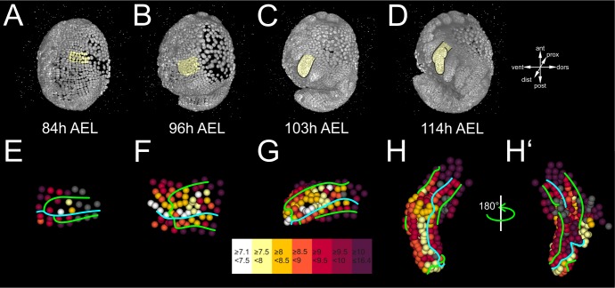
Figure 6.
Differential cell proliferation rates in the Parhyale thoracic limb (see also Figure 6u2014figure supplements 1 and 2 ).
( Au2013D ) Lateral views of the same Parhyale embryo shown in Figure 4 . ( Eu2013Hu2019 ) Tracked cells in limb#1 were color-coded by their average cell cycle length according to the scale (in hours)...
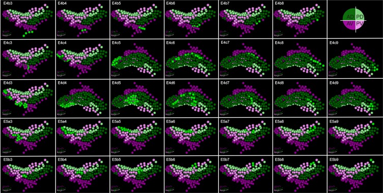
Figure 6u2014figure supplement 1.
Digital clonal analysis in the Parhyale thoracic limb.
Digital clones for each one of the 34 founder cells of the T2 limb#1 visualized at 114 hr (h) after egg-lay (AEL). In each panel, the name of the founder cell is shown in the top left corner and its p...
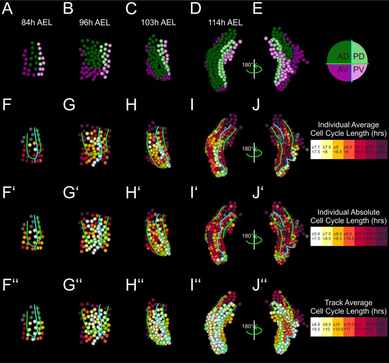
Figure 6u2014figure supplement 2.
Alternative quantifications of cell proliferation rates in the Parhyale thoracic limb.
( A u2013E ) Tracked cells making up the T2 limb#1 shown at the indicated hours (h) after egg-lay (AEL) and color-coded by their compartmental identity: Anterior-Dorsal in dark green, Anterior-Ventral...
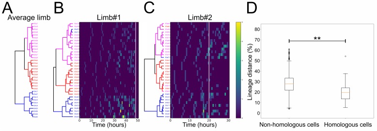
Figure 7.
Lineage comparisons within and across Parhyale thoracic limbs (see also Figure 7u2014source data 1 ).
( A ) Hierarchical clustering of the 34 founder cells in the Parhyale T2 limb based on a distance matrix computed from their average division patterns in limb#1 and limb#2. The cluster of E4c3-c7 and ...
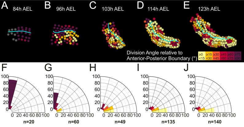
Figure 8.
Oriented cell divisions in the Parhyale thoracic limb.
( Au2013E ) Cells in the T2 limb#1 shown at the indicated hours (h) after egg-lay (AEL) color-coded by the orientation of mitotic divisions relative to the AP boundary (cyan line). The AP boundary is ...
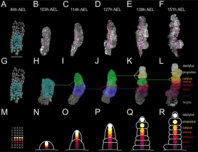
Figure 9.
Elaboration of the Parhyale limb PD axis (see also Figure 9u2014figure supplement 1 ).
( Au2013F ) Rendering of the T2 limb#1 at the indicated hours (h) after egg-lay (AEL). The cells contributing to the T2 primordium are shown in cyan in panel A. Magenta dots indicate the tracked cells...
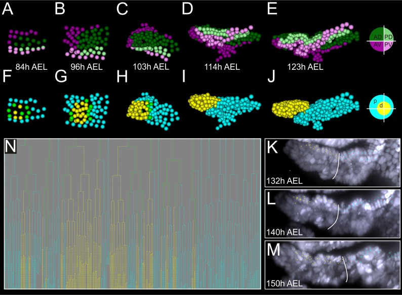
Figure 9u2014figure supplement 1.
Proximal-distal lineage separation in the growing Parhyale thoracic limb.
( Au2013E ) Tracked cells contributing to the T2 limb#1 color-coded by their compartmental identity: Anterior-Dorsal (dark green), Anterior-Ventral (dark magenta), Posterior-Dorsal (light green), and ...
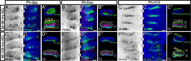
Figure 10.
Analysis of developmental regulatory genes corroborates cellular models of limb morphogenesis (see also Figure 10u2014figure supplement 1 ).
( Au2013F ) Brightfield images of T2, T3 and T4 limbs from S16-S18 embryos (top row, 84u201396 hr AEL) and S19 embryos (bottom row, 96u2013108 hr AEL) stained by in situ hybridization for Ph-dpp (left...
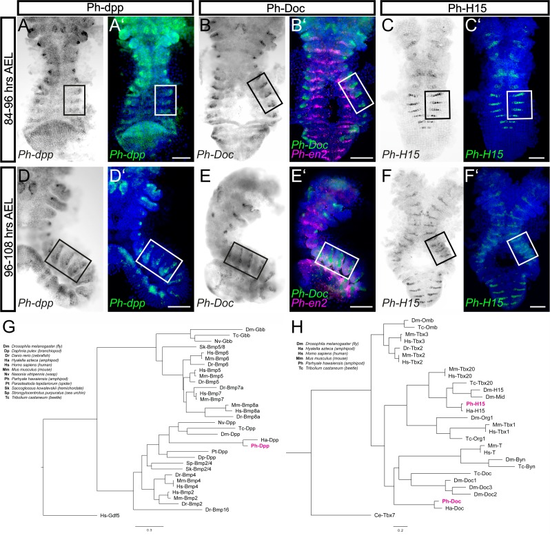
Figure 10u2014figure supplement 1.
Expression of Ph-dpp , Ph-Doc and Ph-H15 during Parhyale limb bud formation.
( Au2013F ) Brightfield images of S16-S18 embryos (top row, 84u201396 hr AEL) and S19 embryos (middle row, 96u2013108 hr AEL) stained by in situ hybridization for Ph-dpp (left columns), Ph-Doc (middle...
Figure images are served from the NIH/NLM PubMed Central Open Access Subset or Europe PMC; copyright remains with the publishers and authors.
💬 Discussion
0 commentsNo comments yet. Be the first to start a discussion!
Leave a Comment