Abstract
AbstractThe hippocampus is essential for spatial and episodic memory but is damaged early in Alzheimer’s disease and is very sensitive to hypoxia. Understanding how it regulates its oxygen supply is therefore key for designing interventions to preserve its function. However, studies of neurovascular function in the hippocampus in vivo have been limited by its relative inaccessibility. Here we compared hippocampal and visual cortical neurovascular function in awake mice, using two photon imaging of individual neurons and vessels and measures of regional blood flow and haemoglobin oxygenation. We show that blood flow, blood oxygenation and neurovascular coupling were decreased in the hippocampus compared to neocortex, because of differences in both the vascular network and pericyte and endothelial cell function. Modelling oxygen diffusion indicates that these features of the hippocampal vasculature may restrict oxygen availability and could explain its sensitivity to damage during neurological conditions, including Alzheimer’s disease, where the brain’s energy supply is decreased.
🔬 Techniques
🔭 Microscopes
💻 Software
✨ Fluorophores
🧪 Sample Preparation
🔬 Cell Lines
🏭 Microscope Brands
🧪 Reagent Suppliers
🔴 Lasers
💻 Software Details
💾 Data Repositories
🏛️ Research Organizations (ROR)
Affiliated research institutions:
📋 Methods
Animal procedures
All experimental procedures were conducted in accordance with the 1986 Animal (Scientific Procedures) Act, with the approval of the UK Home Office and the University of Sussex animal welfare ethical review board. All experiments used mice with a C57BL/6 J background of either sex, which were either wild types (six in total, four males, two females) or expressed GCaMP6f under the control of the Thy1 promoter (C57BL/6J-Tg(Thy1-GCaMP6f)GP5.5Dkim/J 13 ; 30 in total, 15 males, 15 females) and/or DsRed under the control of the NG2 promoter (NG2DsRedBAC 49 ; 17 total, nine males, eight females). Mice were housed in a 12 h reverse dark/light cycle environment at a temperature of 22 °C, with food and water freely available. Surgery for cranial window placement: All mice used for in vivo imaging experiments underwent the following surgical procedure under isoflurane anaesthesia (maintained between 0.8 and 2%). The mouse was secured on a stereotaxic frame with a head mount (Kopf). At the beginning of the surgery mice were subcutaneously injected with 2.4 μl/g of dexamethasone (2 mg/ml), 400 μl of saline and 1.6 μl/g of buprenorphine (0.3 mg/ml, diluted 1:10 with saline) to reduce inflammation, dehydration and post-operative pain, respectively. The temperature was maintained at 37 °C throughout using a homeothermic blanket (PhysioSuite, Kent Scientific Corporation). First, the scalp and underlying thin periosteum layer were removed across the entire dorsal skull surface, and a 3 mm circle overlaying the V1 or HC was marked. Scratches were made in the exposed skull using a scalpel to increase the surface area for bonding with the head plate. The skin around the exposed skull was sealed using dripping tissue adhesive (3 M VetBond). The mouse was then tilted on the head mount so that the area marked for the craniotomy laid flat. Black dental cement (Unifast Powder mixed with black ink (1:15 w/w ) and Unifast Liquid) was applied to all areas of the exposed skull, except the marked craniotomy region and its immediate surround. A custom-made stainless-steel head plate was placed over the dental cement and left for a few minutes until dry. Next, a craniotomy was performed over the previously marked area using a dental drill (Fine Science Tools, burr size 007), after which the underlying dura was carefully removed. For V1 surgeries, an optical window (made from two 3 mm glass coverslips and a 5 mm glass coverslip (Harvard Apparatus) bonded together with optical adhesive (Norland Products, Inc)) was placed into the craniotomy and secured using dripping tissue adhesive and dental cement 50 . For hippocampal surgeries, ~1.3 mm of cortex was aspirated (New Askir 30, CA-MI Srl) until the striations of the corpus callosum (just above CA1 HC) were visible 11 . A 3 mm round stainless-steel cannula (2.4 mm ID, 3 mm OD, 1.5 mm height, Coopers Needle Works Ltd) with a 3 mm glass coverslip (Harvard Apparatus) attached using optical adhesive was inserted into the craniotomy and secured with dripping tissue adhesive and dental cement (secured at the skull surface, above which ~0.2 mm of cannula protruded into the dental cement). The mouse was then injected with 5 μl/g of meloxicam (5 mg/ml, solution for injection, diluted 1:10 with saline) subcutaneously to further aid with post-operative pain relief. Finally, for both surgery types, two rubber rings were secured on top of the head plate with dental cement to allow for two-photon imaging using a water-based objective. The mouse was removed from the head mount attached to the isoflurane machine and placed into a heat box (37 °C) to recover, before being singly housed in a recovery cage. Post-surgery meloxicam (200 μl, 1.5 mg/ml) was administered orally in the food for 3 days for additional pain relief during recovery. Habituation: Prior to imaging, and following a post-surgery recovery period of at least one week, mice were habituated to head fixation on a polystyrene cylinder daily (over the course of 5 days). For the first habituation session, mice were handled by the experimenter and allowed to explore the cylinder freely without head fixation. The following sessions consisted of head-fixing the mouse atop of the cylinder for gradually increasing time periods (increasing from 1 minute in session 2–15 min in session 5). In vivo imaging Experimental set-up: Mice were imaged following a suitable recovery period post-surgery (average number of recovery days in HC: 43 ± 6, and V1: 35 ± 4). For imaging, mice were head-fixed atop of a polystyrene cylinder, fitted with a Kuebler rotary encoder (4096 steps/revolution) to measure locomotion, underneath a two-photon microscope (Scientifica) or combined laser doppler flowmetry/haemoglobin spectroscopy probe (VMS-Oxy, Moor Instruments; Fig. 1c ). In front of the mice were two computer screens which, when required, displayed a virtual reality maze (custom-designed in ViRMEn 51 , MATLAB; for HC surgery mice; Fig. 1e ) or drifting gratings (PsychoPy, 315° orientation refreshed at 60 frames per second; for V1 surgery mice; Fig. 1f ). Combined laser doppler flowmetry/haemoglobin spectroscopy (Oxy-CBF probe) : A combined laser doppler flowmetry/haemoglobin spectroscopy probe (Moor Instruments, VMS-Oxy) allowed for monitoring (at 40 Hz) of the following net haemodynamic measures via VMS4.0 software: blood flow (flux), speed, oxygenated haemoglobin (HbO), deoxygenated haemoglobin (Hbr), total haemoglobin (Hbt, Hbt = HbO + Hbr) and oxygen saturation (SO 2 , SO 2 = HbO/(HbO + Hbr)). Except for SO 2 , which is expressed as a percentage of 100% saturation, these measurements are expressed in arbitrary units as we cannot calculate absolute flow rates and haemoglobin concentrations from these data. Experiments typically lasted 0.5–1 h. The CMRO 2 over time ( t ) was estimated from these variables using Eq. ( 1 ) 52 : 1 documentclass[12pt]{minimal} usepackage{amsmath} usepackage{wasysym} usepackage{amsfonts} usepackage{amssymb} usepackage{amsbsy} usepackage{mathrsfs} usepackage{upgreek} setlength{oddsidemargin}{-69pt} begin{document}$${{{{rm{CMRO}}}}_{2}}(t)={{{rm{CBF}}}},(t),times frac{{{{rm{Hbr}}}},(t)}{{{{rm{Hbt}}}},(t)}$$end{document} CMRO 2 ( t ) = CBF ( t ) × Hbr ( t ) Hbt ( t ) Laser doppler flowmetry is commonly used to compare relative not absolute differences in flow, but we reasoned that if we could discount potential artefactual contributions to the LDF signal 53 , differences in the signal between regions might be informative about regional differences in CBF. First, we checked whether probe placement across sessions affected signal variability. We plotted the responses recorded on different sessions within the same animal and between animals (Supplementary Figure 10 ). We then compared the standard deviation for each mouse (with ≥2 recording sessions, N = 6 mice for HC, N = 7 mice for V1) between measurements and across regions and compared variability between regions. There was no difference in inter-session standard deviation between brain regions for any of the haemodynamic measures (independent sample t tests; p > 0.19). Variability in CBF was greater than that of haemoglobin absorbance recorded using spectroscopy, possibly reflecting differences in probe placement (e.g., over large pial vessels) and spatial variability in perfusion. Nevertheless, there were no significant differences between recordings obtained within a region (V1 or HC), whereas the difference between regions was significant (Fig. 2b ). We also checked that fluorescence signals from the brain did not interfere with the haemodynamic measurements and reached zero in the absence of blood flow following the death of the subject (Supplementary Figure 10 ). Finally, we considered the possible effects of the large sampling volume of our LDF probe on our results. It has a 500 μm separation between the transmission and detection fibres and a wavelength of 780 nm, so samples deep in the tissue, with a median signal depth of around 0.9 mm and a maximum depth of 2 mm 54 . Thus, some of the signal recorded in V1 comes from underlying corpus callosum and HC, and some of that recorded from HC originates in the thalamus. However, it is highly unlikely that signal from these areas could produce the regional differences we report here, as corpus callosum and HC have low vascular densities so cannot be boosting the apparent V1 CBF signal, whereas the thalamus has a high vascular density 15 so will not be artificially reducing the signal attributed to HC. Analysis of oxy-CBF probe data : The oxy-CBF probe data (flux, speed, SO 2 , HbO, Hbr, Hbt or CMRO 2 ) was categorised as occurring during periods of rest (i.e., no locomotion and no visual screen presentations) or not. The average value of each haemodynamic parameter was calculated per animal (across sessions) during these stationary periods (Fig. 2a–c ). Peaks in the CMRO 2 trace were detected (as specified in the section below: ‘Analysis of two-photon microscopy data’, Fig. 5f, h ), and those peaks which were more than two standard deviations larger than their preceding baseline were extracted, along with their corresponding Hbt traces (Fig. 5g, i ). Two-photon microscopy : In order to visualise blood vessels during imaging mice were injected with 2.5% (w/v) Texas Red Dextran dissolved in saline (70 kDa via tail vein or 3 kDa subcutaneously, Fisher Scientific) alone or in combination with fluorescein Dextran dissolved in saline (70 kDa via tail vein, Fisher Scientific). All blood vessels recorded local to neuronal calcium activity were capillaries, precapillary arterioles or arteriole branches to ensure that similar types of vessels were selected between the regions. High-resolution imaging of vessels and calcium from excitatory neurons was performed with a commercial two-photon microscope (Scientifica), a high numerical aperture water-dipping objective (×20 aperture, XLUMPlanFL N, Olympus or ×16 aperture, LWD, Nikon), and a Chameleon Vision II Ti:Sapphire laser (Coherent). Tissue was excited at 940 nm, and the emitted light was filtered to collect red and green light from Texas Red Dextran (vessel lumen) and Thy1-GCaMP6f (excitatory neurons), respectively. Imaging sessions were recorded in SciScan software (SciScan v1.2.1, Scientifica). Typically, imaging occurred up to a depth of ~500 μm from the surface. Imaging sessions included both wide field-of-view recordings of network neuronal calcium activity (256 × 256 pixels, speed range 6.10–15.26 Hz, speed average 7.75 Hz, pixel size range 1.35–2.56 μm, pixel size average 1.80 μm), and smaller field-of-view recordings of individual blood vessels and local neuronal calcium signalling (256 × 256 pixels, speed range 3.05–7.63 Hz, speed average 6.64 Hz; pixel size range 0.15–0.63 μm, pixel size average 0.23 μm). High speed line scans (speed range 413–2959 Hz, speed average 1092 Hz; pixel size range 0.15–0.46 μm, pixel size average 0.20 μm) were also taken from individual blood vessels to track diameter, RBC velocity, RBC flux and haematocrit from capillaries, and sometimes the line scan path also passed through a nearby neuron (for concurrent calcium readings). Vessels and local calcium were imaged from each of the distinct layers of CA1 (stratum oriens, stratum pyramidale, stratum radiatum, stratum lacunosum–moleculare) and V1 (L1, L2/3, L4). The layers in CA1 were clearly distinguishable by the changing morphology of the pyramidal neurons over increasing depths within this region 55 (Fig. 1b). The layers of V1 were distinguished based on the distance of the imaging site from the pial vessels 56 . Two-photon imaging experiments typically lasted 1–3 h. Analysis of two-photon microscopy data : Excitatory calcium activity was first registered in ImageJ to correct motion artefacts, before being extracted using the CellSort package in MATLAB 57 . CellSort identified regions of interest (ROIs) over multiple active individual cells (both soma and NP). Any ROIs that overlapped the same cell were either merged or removed, as appropriate. For most analyses, net activity in a recording was calculated across ROIs, except when correlations between individual ROIs were calculated (Fig. 5c ). Vessel diameter (XY movies and line scans) and RBC velocity, flux and haematocrit (line scans) data were registered in ImageJ to remove motion artefacts and despeckled. The vascular lumen was bright due to the dye injection, whereas the RBCs within the vessel and background around the vessel were dark. Custom MATLAB scripts were used to extract the diameter along the vessel branch(es), or the RBC velocity, flux or haematocrit. In brief, for each frame of XY movies the vessel was skeletonised, meaning its length was eroded to generate a single-pixel diameter line running through the entire length of the vessel at its centre. The intensity profile of a line perpendicular to this vessel axis was taken at every other pixel along the length of this skeleton, averaged across a running window of five pixels. The diameter was calculated from the full-width half maximum of this intensity profile. For RBC velocity data from line scans, we adapted freely available code 58 . In short, the angle of the shadow cast by the RBCs travelling through the vessel was used to calculate the speed at which they travelled over successive 40 ms (time, t ) blocks (with an overlap of 10 ms in time (i.e. t/4) between blocks). For RBC flux data from line scans, the number of RBCs per second was counted using an automated script in MATLAB. In brief, two-photon recordings were binarized. An average intensity curve was generated for the centre of binarized scan, and groups of dark pixels (RBCs) fell below a minimum threshold, which allowed for them to be counted within a 250 ms time window. The accuracy of the automated RBC counter was also verified by checking for consistency with a subset of the data which was manually counted. For calculating haematocrit values within a capillary over time, again line scan recordings were binarized, and the percentage of overall dark space (i.e., containing RBCs) was calculated over successive 40 ms blocks with an overlap of 10 ms in time. To detect peaks in the neuronal calcium signal local to a blood vessel, the calcium trace was first normalised across the entire recording (e.g., Figure 3b ) using Eq. ( 2 ), before identifying putative events as peaks that were >10% of the maximum. The data around each calcium peak was then extracted from the raw (unnormalized) trace (5 s before and 10 s after), and these peaks were then normalised to their own baseline (5 s preceding peak) using Eq. ( 3 ). Changes in calcium fluorescence from baseline (e.g., Figure 3d, j ) are presented as Δ F / F . Delta is conventionally used to denote a change from the initial state, and so delta F over F compares the change of intensity after activation to that at resting baseline. 2 documentclass[12pt]{minimal} usepackage{amsmath} usepackage{wasysym} usepackage{amsfonts} usepackage{amssymb} usepackage{amsbsy} usepackage{mathrsfs} usepackage{upgreek} setlength{oddsidemargin}{-69pt} begin{document}$$Delta {F}/{F}=frac{F-{F_{{{rm{min}}}}}}{F_{{{rm{max}}}}-{F_{{{rm{min}}}}}}$$end{document} Δ F / F = F − F min F max − F min 3 documentclass[12pt]{minimal} usepackage{amsmath} usepackage{wasysym} usepackage{amsfonts} usepackage{amssymb} usepackage{amsbsy} usepackage{mathrsfs} usepackage{upgreek} setlength{oddsidemargin}{-69pt} begin{document}$$Delta {F}/{F}=frac{F-F_{0}}{{{{rm{abs}}}}({{{rm{F}}}}_{0})}$$end{document} Δ F / F = F − F 0 abs ( F 0 ) F represents the entire fluorescence trace, and F 0 represents the baseline fluorescence period. Events were excluded if their peaks were smaller than two standard deviations above the mean value of the baseline. Vessel traces were extracted across the times of these calcium events, or after bootstrapping by shuffling each of the vessel traces over 100 iterations across time using the MATLAB function randperm, so they were no longer aligned to calcium events. For every calcium event, both the corresponding real vessel diameter trace and shuffled vessel diameter trace were classified as being responsive or not. Responsive diameter traces were those where dilations occurred for >0.5 s, within 5 s of the calcium event, that were >1 standard deviation above baseline. Behavioural testing : Animals that had previously undergone HC or V1 surgery for in vivo imaging underwent a simple hippocampal-dependent object location memory task to test spatial memory 59 (Supplementary Figure 6 ). The mouse was presented with two objects in a training environment for 10 min, before being removed from the environment. After 5 min in the home cage, the mouse was then returned to the environment, after one of the objects had been moved to a novel location. The time spent exploring both the familiar and novel object locations was assessed by a blinded observer hand-scoring the time per object. Any mice which spent less than total 5 s exploring the test environment were excluded from the analysis.
Show full methods section
Animal procedures
All experimental procedures were conducted in accordance with the 1986 Animal (Scientific Procedures) Act, with the approval of the UK Home Office and the University of Sussex animal welfare ethical review board. All experiments used mice with a C57BL/6 J background of either sex, which were either wild types (six in total, four males, two females) or expressed GCaMP6f under the control of the Thy1 promoter (C57BL/6J-Tg(Thy1-GCaMP6f)GP5.5Dkim/J 13 ; 30 in total, 15 males, 15 females) and/or DsRed under the control of the NG2 promoter (NG2DsRedBAC 49 ; 17 total, nine males, eight females). Mice were housed in a 12 h reverse dark/light cycle environment at a temperature of 22 °C, with food and water freely available. Surgery for cranial window placement: All mice used for in vivo imaging experiments underwent the following surgical procedure under isoflurane anaesthesia (maintained between 0.8 and 2%). The mouse was secured on a stereotaxic frame with a head mount (Kopf). At the beginning of the surgery mice were subcutaneously injected with 2.4 μl/g of dexamethasone (2 mg/ml), 400 μl of saline and 1.6 μl/g of buprenorphine (0.3 mg/ml, diluted 1:10 with saline) to reduce inflammation, dehydration and post-operative pain, respectively. The temperature was maintained at 37 °C throughout using a homeothermic blanket (PhysioSuite, Kent Scientific Corporation). First, the scalp and underlying thin periosteum layer were removed across the entire dorsal skull surface, and a 3 mm circle overlaying the V1 or HC was marked. Scratches were made in the exposed skull using a scalpel to increase the surface area for bonding with the head plate. The skin around the exposed skull was sealed using dripping tissue adhesive (3 M VetBond). The mouse was then tilted on the head mount so that the area marked for the craniotomy laid flat. Black dental cement (Unifast Powder mixed with black ink (1:15 w/w ) and Unifast Liquid) was applied to all areas of the exposed skull, except the marked craniotomy region and its immediate surround. A custom-made stainless-steel head plate was placed over the dental cement and left for a few minutes until dry. Next, a craniotomy was performed over the previously marked area using a dental drill (Fine Science Tools, burr size 007), after which the underlying dura was carefully removed. For V1 surgeries, an optical window (made from two 3 mm glass coverslips and a 5 mm glass coverslip (Harvard Apparatus) bonded together with optical adhesive (Norland Products, Inc)) was placed into the craniotomy and secured using dripping tissue adhesive and dental cement 50 . For hippocampal surgeries, ~1.3 mm of cortex was aspirated (New Askir 30, CA-MI Srl) until the striations of the corpus callosum (just above CA1 HC) were visible 11 . A 3 mm round stainless-steel cannula (2.4 mm ID, 3 mm OD, 1.5 mm height, Coopers Needle Works Ltd) with a 3 mm glass coverslip (Harvard Apparatus) attached using optical adhesive was inserted into the craniotomy and secured with dripping tissue adhesive and dental cement (secured at the skull surface, above which ~0.2 mm of cannula protruded into the dental cement). The mouse was then injected with 5 μl/g of meloxicam (5 mg/ml, solution for injection, diluted 1:10 with saline) subcutaneously to further aid with post-operative pain relief. Finally, for both surgery types, two rubber rings were secured on top of the head plate with dental cement to allow for two-photon imaging using a water-based objective. The mouse was removed from the head mount attached to the isoflurane machine and placed into a heat box (37 °C) to recover, before being singly housed in a recovery cage. Post-surgery meloxicam (200 μl, 1.5 mg/ml) was administered orally in the food for 3 days for additional pain relief during recovery. Habituation: Prior to imaging, and following a post-surgery recovery period of at least one week, mice were habituated to head fixation on a polystyrene cylinder daily (over the course of 5 days). For the first habituation session, mice were handled by the experimenter and allowed to explore the cylinder freely without head fixation. The following sessions consisted of head-fixing the mouse atop of the cylinder for gradually increasing time periods (increasing from 1 minute in session 2–15 min in session 5). In vivo imaging Experimental set-up: Mice were imaged following a suitable recovery period post-surgery (average number of recovery days in HC: 43 ± 6, and V1: 35 ± 4). For imaging, mice were head-fixed atop of a polystyrene cylinder, fitted with a Kuebler rotary encoder (4096 steps/revolution) to measure locomotion, underneath a two-photon microscope (Scientifica) or combined laser doppler flowmetry/haemoglobin spectroscopy probe (VMS-Oxy, Moor Instruments; Fig. 1c ). In front of the mice were two computer screens which, when required, displayed a virtual reality maze (custom-designed in ViRMEn 51 , MATLAB; for HC surgery mice; Fig. 1e ) or drifting gratings (PsychoPy, 315° orientation refreshed at 60 frames per second; for V1 surgery mice; Fig. 1f ). Combined laser doppler flowmetry/haemoglobin spectroscopy (Oxy-CBF probe) : A combined laser doppler flowmetry/haemoglobin spectroscopy probe (Moor Instruments, VMS-Oxy) allowed for monitoring (at 40 Hz) of the following net haemodynamic measures via VMS4.0 software: blood flow (flux), speed, oxygenated haemoglobin (HbO), deoxygenated haemoglobin (Hbr), total haemoglobin (Hbt, Hbt = HbO + Hbr) and oxygen saturation (SO 2 , SO 2 = HbO/(HbO + Hbr)). Except for SO 2 , which is expressed as a percentage of 100% saturation, these measurements are expressed in arbitrary units as we cannot calculate absolute flow rates and haemoglobin concentrations from these data. Experiments typically lasted 0.5–1 h. The CMRO 2 over time ( t ) was estimated from these variables using Eq. ( 1 ) 52 : 1 documentclass[12pt]{minimal} usepackage{amsmath} usepackage{wasysym} usepackage{amsfonts} usepackage{amssymb} usepackage{amsbsy} usepackage{mathrsfs} usepackage{upgreek} setlength{oddsidemargin}{-69pt} begin{document}$${{{{rm{CMRO}}}}_{2}}(t)={{{rm{CBF}}}},(t),times frac{{{{rm{Hbr}}}},(t)}{{{{rm{Hbt}}}},(t)}$$end{document} CMRO 2 ( t ) = CBF ( t ) × Hbr ( t ) Hbt ( t ) Laser doppler flowmetry is commonly used to compare relative not absolute differences in flow, but we reasoned that if we could discount potential artefactual contributions to the LDF signal 53 , differences in the signal between regions might be informative about regional differences in CBF. First, we checked whether probe placement across sessions affected signal variability. We plotted the responses recorded on different sessions within the same animal and between animals (Supplementary Figure 10 ). We then compared the standard deviation for each mouse (with ≥2 recording sessions, N = 6 mice for HC, N = 7 mice for V1) between measurements and across regions and compared variability between regions. There was no difference in inter-session standard deviation between brain regions for any of the haemodynamic measures (independent sample t tests; p > 0.19). Variability in CBF was greater than that of haemoglobin absorbance recorded using spectroscopy, possibly reflecting differences in probe placement (e.g., over large pial vessels) and spatial variability in perfusion. Nevertheless, there were no significant differences between recordings obtained within a region (V1 or HC), whereas the difference between regions was significant (Fig. 2b ). We also checked that fluorescence signals from the brain did not interfere with the haemodynamic measurements and reached zero in the absence of blood flow following the death of the subject (Supplementary Figure 10 ). Finally, we considered the possible effects of the large sampling volume of our LDF probe on our results. It has a 500 μm separation between the transmission and detection fibres and a wavelength of 780 nm, so samples deep in the tissue, with a median signal depth of around 0.9 mm and a maximum depth of 2 mm 54 . Thus, some of the signal recorded in V1 comes from underlying corpus callosum and HC, and some of that recorded from HC originates in the thalamus. However, it is highly unlikely that signal from these areas could produce the regional differences we report here, as corpus callosum and HC have low vascular densities so cannot be boosting the apparent V1 CBF signal, whereas the thalamus has a high vascular density 15 so will not be artificially reducing the signal attributed to HC. Analysis of oxy-CBF probe data : The oxy-CBF probe data (flux, speed, SO 2 , HbO, Hbr, Hbt or CMRO 2 ) was categorised as occurring during periods of rest (i.e., no locomotion and no visual screen presentations) or not. The average value of each haemodynamic parameter was calculated per animal (across sessions) during these stationary periods (Fig. 2a–c ). Peaks in the CMRO 2 trace were detected (as specified in the section below: ‘Analysis of two-photon microscopy data’, Fig. 5f, h ), and those peaks which were more than two standard deviations larger than their preceding baseline were extracted, along with their corresponding Hbt traces (Fig. 5g, i ). Two-photon microscopy : In order to visualise blood vessels during imaging mice were injected with 2.5% (w/v) Texas Red Dextran dissolved in saline (70 kDa via tail vein or 3 kDa subcutaneously, Fisher Scientific) alone or in combination with fluorescein Dextran dissolved in saline (70 kDa via tail vein, Fisher Scientific). All blood vessels recorded local to neuronal calcium activity were capillaries, precapillary arterioles or arteriole branches to ensure that similar types of vessels were selected between the regions. High-resolution imaging of vessels and calcium from excitatory neurons was performed with a commercial two-photon microscope (Scientifica), a high numerical aperture water-dipping objective (×20 aperture, XLUMPlanFL N, Olympus or ×16 aperture, LWD, Nikon), and a Chameleon Vision II Ti:Sapphire laser (Coherent). Tissue was excited at 940 nm, and the emitted light was filtered to collect red and green light from Texas Red Dextran (vessel lumen) and Thy1-GCaMP6f (excitatory neurons), respectively. Imaging sessions were recorded in SciScan software (SciScan v1.2.1, Scientifica). Typically, imaging occurred up to a depth of ~500 μm from the surface. Imaging sessions included both wide field-of-view recordings of network neuronal calcium activity (256 × 256 pixels, speed range 6.10–15.26 Hz, speed average 7.75 Hz, pixel size range 1.35–2.56 μm, pixel size average 1.80 μm), and smaller field-of-view recordings of individual blood vessels and local neuronal calcium signalling (256 × 256 pixels, speed range 3.05–7.63 Hz, speed average 6.64 Hz; pixel size range 0.15–0.63 μm, pixel size average 0.23 μm). High speed line scans (speed range 413–2959 Hz, speed average 1092 Hz; pixel size range 0.15–0.46 μm, pixel size average 0.20 μm) were also taken from individual blood vessels to track diameter, RBC velocity, RBC flux and haematocrit from capillaries, and sometimes the line scan path also passed through a nearby neuron (for concurrent calcium readings). Vessels and local calcium were imaged from each of the distinct layers of CA1 (stratum oriens, stratum pyramidale, stratum radiatum, stratum lacunosum–moleculare) and V1 (L1, L2/3, L4). The layers in CA1 were clearly distinguishable by the changing morphology of the pyramidal neurons over increasing depths within this region 55 (Fig. 1b). The layers of V1 were distinguished based on the distance of the imaging site from the pial vessels 56 . Two-photon imaging experiments typically lasted 1–3 h. Analysis of two-photon microscopy data : Excitatory calcium activity was first registered in ImageJ to correct motion artefacts, before being extracted using the CellSort package in MATLAB 57 . CellSort identified regions of interest (ROIs) over multiple active individual cells (both soma and NP). Any ROIs that overlapped the same cell were either merged or removed, as appropriate. For most analyses, net activity in a recording was calculated across ROIs, except when correlations between individual ROIs were calculated (Fig. 5c ). Vessel diameter (XY movies and line scans) and RBC velocity, flux and haematocrit (line scans) data were registered in ImageJ to remove motion artefacts and despeckled. The vascular lumen was bright due to the dye injection, whereas the RBCs within the vessel and background around the vessel were dark. Custom MATLAB scripts were used to extract the diameter along the vessel branch(es), or the RBC velocity, flux or haematocrit. In brief, for each frame of XY movies the vessel was skeletonised, meaning its length was eroded to generate a single-pixel diameter line running through the entire length of the vessel at its centre. The intensity profile of a line perpendicular to this vessel axis was taken at every other pixel along the length of this skeleton, averaged across a running window of five pixels. The diameter was calculated from the full-width half maximum of this intensity profile. For RBC velocity data from line scans, we adapted freely available code 58 . In short, the angle of the shadow cast by the RBCs travelling through the vessel was used to calculate the speed at which they travelled over successive 40 ms (time, t ) blocks (with an overlap of 10 ms in time (i.e. t/4) between blocks). For RBC flux data from line scans, the number of RBCs per second was counted using an automated script in MATLAB. In brief, two-photon recordings were binarized. An average intensity curve was generated for the centre of binarized scan, and groups of dark pixels (RBCs) fell below a minimum threshold, which allowed for them to be counted within a 250 ms time window. The accuracy of the automated RBC counter was also verified by checking for consistency with a subset of the data which was manually counted. For calculating haematocrit values within a capillary over time, again line scan recordings were binarized, and the percentage of overall dark space (i.e., containing RBCs) was calculated over successive 40 ms blocks with an overlap of 10 ms in time. To detect peaks in the neuronal calcium signal local to a blood vessel, the calcium trace was first normalised across the entire recording (e.g., Figure 3b ) using Eq. ( 2 ), before identifying putative events as peaks that were >10% of the maximum. The data around each calcium peak was then extracted from the raw (unnormalized) trace (5 s before and 10 s after), and these peaks were then normalised to their own baseline (5 s preceding peak) using Eq. ( 3 ). Changes in calcium fluorescence from baseline (e.g., Figure 3d, j ) are presented as Δ F / F . Delta is conventionally used to denote a change from the initial state, and so delta F over F compares the change of intensity after activation to that at resting baseline. 2 documentclass[12pt]{minimal} usepackage{amsmath} usepackage{wasysym} usepackage{amsfonts} usepackage{amssymb} usepackage{amsbsy} usepackage{mathrsfs} usepackage{upgreek} setlength{oddsidemargin}{-69pt} begin{document}$$Delta {F}/{F}=frac{F-{F_{{{rm{min}}}}}}{F_{{{rm{max}}}}-{F_{{{rm{min}}}}}}$$end{document} Δ F / F = F − F min F max − F min 3 documentclass[12pt]{minimal} usepackage{amsmath} usepackage{wasysym} usepackage{amsfonts} usepackage{amssymb} usepackage{amsbsy} usepackage{mathrsfs} usepackage{upgreek} setlength{oddsidemargin}{-69pt} begin{document}$$Delta {F}/{F}=frac{F-F_{0}}{{{{rm{abs}}}}({{{rm{F}}}}_{0})}$$end{document} Δ F / F = F − F 0 abs ( F 0 ) F represents the entire fluorescence trace, and F 0 represents the baseline fluorescence period. Events were excluded if their peaks were smaller than two standard deviations above the mean value of the baseline. Vessel traces were extracted across the times of these calcium events, or after bootstrapping by shuffling each of the vessel traces over 100 iterations across time using the MATLAB function randperm, so they were no longer aligned to calcium events. For every calcium event, both the corresponding real vessel diameter trace and shuffled vessel diameter trace were classified as being responsive or not. Responsive diameter traces were those where dilations occurred for >0.5 s, within 5 s of the calcium event, that were >1 standard deviation above baseline. Behavioural testing : Animals that had previously undergone HC or V1 surgery for in vivo imaging underwent a simple hippocampal-dependent object location memory task to test spatial memory 59 (Supplementary Figure 6 ). The mouse was presented with two objects in a training environment for 10 min, before being removed from the environment. After 5 min in the home cage, the mouse was then returned to the environment, after one of the objects had been moved to a novel location. The time spent exploring both the familiar and novel object locations was assessed by a blinded observer hand-scoring the time per object. Any mice which spent less than total 5 s exploring the test environment were excluded from the analysis.
Ex vivo imaging
Transcardial perfusion and gel-filling the vasculature : Adult mice were terminally anaesthetised with pentobarbital. A transcardial perfusion was performed using 4% paraformaldehyde (PFA) in 0.1 M phosphate buffer solution (PBS). In cases where the vasculature was labelled, this was also followed by the perfusion of 5% gelatin containing 0.2% fluorescein isothiocyanate (FITC)-conjugated albumin. Mice were then chilled on ice for at least 30 min, before brains were extracted and fixed in 4% PFA overnight. The brains were subsequently transferred to a 30% sucrose solution in PBS with 0.1% sodium azide for a minimum of 3 days, after which they were sliced (200 μm slices) on a vibratome (Leica), and stored in the fridge (at 4 °C) in PBS with 0.1% sodium azide, before immunohistochemical labelling and/or mounting. Immunohistochemical labelling and slice mounting : Adult NG2-DsRed mice were used for pericyte morphology and vascular network analyses (Figs. 2 and 6 ), as pericytes and SMCs were transgenically labelled in red. Vessel type could therefore be identified based on the smooth muscle or pericyte cell morphology. Adult wild-type or NG2-DsRed mice, which had previously undergone CA1 surgery for two-photon imaging, were used for vascular network analysis on the surgical versus the control hemisphere, and adult Thy1-GCaMP6f mice, which had also previously undergone CA1 surgery, were used for the analysis of CA1 area on surgical and control hemispheres (i.e., following cannula insertion/possible compression, Supplementary Figure 5 ). For analysis of inflammation (Supplementary Figure 6 ) mice that had previously undergone HC or V1 surgery for in vivo imaging were used, and active astrocytes were labelled for GFAP and microglia labelled for Iba1 using immunohistochemistry. First, brain slices were washed in 1× PBS whilst being shaken for three cycles (10 min per wash). The slices were then blocked in 5% normal goat serum and 0.3% Triton X-100 in 1× PBS for an hour. Slices were incubated in the relevant primary antibodies (chicken anti-GFAP primary antibody; Abcam, ab4674, 1:500 dilution or rabbit anti-Iba1, WAKO, 019-19741, 1:600 dilution) for 36 h at 4 °C. Slices were washed three times in PBS, before being incubated in the relevant secondary antibody for 24 h at 4 °C (Alexa 647 goat anti-chicken, Abcam, 1:500 dilution or Alexa 647 goat anti-rabbit, Abcam, 1:500 dilution). Gel-filled and/or immunohistochemically labelled slices were washed for a final three cycles in PBS, before being mounted onto slides in Vectashield Hardset mounting medium and stored at 4 °C before imaging. Confocal imaging : Imaging was performed on a confocal microscope (Leica SP8, collected using LAS X software) using a ×20 objective (HC PL APO CS2, 20×/0.75, dry). Continuous wave lasers with ~488, ~543 and ~633 nm excitation wavelengths were used for FITC, DsRed and Alexa 647, respectively. Images were collected with dimensions of 1024 by 1024 pixels (with a lateral resolution of 0.57 μm per pixel), averaged 4–6 times per line, and were viewed and analysed in ImageJ software. Analysing pericyte and vessel morphology : For the analysis of individual pericyte cell morphology, composite z-stacks of brain slices with DsRed-labelled pericytes and FITC-albumin labelled blood vessels were used to identify the span along the vessel length of individual pericyte cells, and the vessel diameter measured at the location of the DsRed-positive cell body. The cell was then categorised as being an ensheathing, mesh or thin-strand pericyte, based on its distinct morphology 18 (see Fig. 6i for example images). To calculate capillary density (Fig. 2d, e , Supplementary Figure 5 ) and vessel diameter by depth from the imaging surface (Fig. 6b ), an in-house ImageJ macro was used to skeletonise 3D stacks of the vasculature, determine all the skeleton coordinates and branch points, and then create distance maps of the vasculature. The capillary density was then calculated by dividing the total length of the vessel skeleton within the region by the tissue volume imaged. The vessel radii were found by determining the grey value from the distance map at each skeleton point. The coordinates of the vessel skeleton were also used to determine the vessel’s depth in the tissue. Analysing post-surgery inflammation levels : For each GFAP- or Iba1-labelled brain slice, the z-stack was 2D maximum-projected for both the surgical and non-surgical hemisphere. In each hemisphere, three linear 500 μm ROIs were placed perpendicularly to the cranial window (or equivalent locations in the non-surgical hemisphere). The intensity profiles along these three lines were then averaged and normalised to the average value in the non-surgical hemisphere of the same slice. Analysing the area of CA1 in surgical and non-surgical hemispheres : Wide-field images were taken of the entire brain slice by tile scanning (Supplementary Figure 5 ). In brief, two positions were marked around the outer edges of the brain slice, one in the upper left corner and one the lower right corner. A rectangle with multiple grids was created between these two positions, and a motorised stage was used to move the sample and create a tiled scan of the whole slice. 2D images were captured at the focal point for each grid, with blending (statistical and linear) between grid images. An ImageJ plugin 60 was then used to stitch the grid images together in post processing. For analysis of the area and aspect ratio of CA1 in surgical and control hemispheres, the freehand tool was used to draw around CA1, and calibrated area and bounding rectangle measurements were generated. The aspect ratio was calculated by dividing the height of the selection by its width, meaning larger values represented a taller/narrower shape, and smaller values a wider/shorter shape.
Single-cell RNA-Seq data
The raw single-cell RNA-Seq data were taken from a freely available online database 17 ( http://linnarssonlab.org/cortex/ ). The authors used quantitative single-cell RNA-Seq to perform a molecular census of cells in somatosensory cortex (S1) and HC (CA1) and categorise cells based on their transcriptome. We compared expression of components of neurovascular signalling pathways, ion channels or contractile machinery in vascular cells (pericytes, SMCs, endothelial cells; Supplementary Figure 8 ) and vasodilatory signalling pathways in pyramidal cells, interneurons, and astrocytes (Fig. 4 ). The levels of target transcripts in HC and cortex were compared using multiple t tests in RStudio, with a Holm–Bonferroni correction for multiple comparisons (see Supplementary Tables 1 – 4 ). Modelling oxygen concentrations in tissue Estimating capillary oxygen concentrations : Our in vivo oxy-CBF probe measurements give us the saturation of oxygen (SO 2 ) in the blood. From SO 2 , we calculated the partial pressure (pO 2 ) of oxygen in RBCs using the haemoglobin oxygen dissociation curve for C57/BL6 mice (the background of our experimental mice), with a Hill coefficient h of 2.59 and a P50 of 40.2 mmHg 61 (4). 4 documentclass[12pt]{minimal} usepackage{amsmath} usepackage{wasysym} usepackage{amsfonts} usepackage{amssymb} usepackage{amsbsy} usepackage{mathrsfs} usepackage{upgreek} setlength{oddsidemargin}{-69pt} begin{document}$${{{{mathrm{sO}}}}_{2}}= frac{{{{{{mathrm{p}}}}{{{mathrm{O}}}}}_2^h}} {{{{{{mathrm{p}}}}{{{mathrm{O}}}}}_2^h} + {{P50}^{h}}}$$end{document} sO 2 = p O 2 h p O 2 h + P 50 h This yielded RBC pO 2 values of 30 mmHg (42 μM at 37 °C) in HC and 43 mmHg (60 μM) in V1. Micromolar concentrations of oxygen in tissue at 37 °C were calculated from partial pressures using a Henry’s Law constant of 1.3 × 10 −5 mol/(m 3 Pa) at standard temperature and pressure, and a temperature conversion factor of 1500 K 62 . Our calculated RBC oxygen levels were consistent with those measured with a phosphorescent probe in somatosensory cortical and olfactory bulb RBCs in an awake mouse (30–100 mmHg) 27 , 41 , in experiments that also measured pO 2 between RBCs (interRBC pO 2 ). We then estimated the interRBC pO 2 for our experiments by using those interRBC phosphorescent probe measurements that had the same pO 2 as we observed 27 , 41 . This yielded an estimate of interRBC [O 2 ] in V1 of 15 mmHg/21 μM and in HC of 10 mmHg/14 μM. Because tissue pO 2 equilibrates with interRBC pO 2 rather than RBC pO 2 27 , we used these estimates of interRBC [O 2 ] as the capillary [O 2 ] in our model. Indeed if we ran our simulations using RBC pO 2 as the capillary [O 2 ], tissue [O 2 ] estimates were impossibly much higher than the expected interRBC [O 2 ] values (reaching 37 µM in HC and 58 µM in V1 with a V max of 3 mM/min), confirming that interRBC rather than intra RBC [O 2 ] levels are likely to be the main drivers of tissue [O 2 ]. Calculating capillary spacings : Using ImageJ (Exact Euclidean Distance Transform (3D) plugin) we calculated a 3D distance map from a smoothed and binarized in vivo z-stack of the vascular network in each brain region. We extracted five substacks of 100 × 100 × 100 μm from each distance map. The distribution of the distances of pixels from the nearest vessel was then extracted and averaged across all substacks from a given larger z-stack (giving an average distance per animal). Histograms of these data were averaged across five stacks per brain region (Fig. 7c ) and the 50th, 95th and intermediate centile distances from a capillary were calculated (Fig. 7e–l, m ). For a given bar in the histogram, contributing pixels are either at a midpoint between two capillaries, or are closer to one capillary than another. Those pixels above the 95th centile must lie more-or-less at the midpoint between vessels, whereas many pixels at the median distance from the vessel will be nearer to one vessel than another. However [O 2 ] at each distance from a vessel would be larger if that point is at the midpoint between two vessels compared with being nearer to one vessel than another (and therefore oxygen from that vessel is having to feed a larger tissue volume). For the diffusion model below, we therefore used the distribution of tissue distances from a capillary as a conservative estimate of capillary separation, meaning that our estimates of levels of oxygen in the tissue are, if anything, slightly overestimated. Diffusion model : We used the Heat Transfer functions in the Partial Differential Equation Toolbox of MATLAB to numerically solve Fick’s diffusion equation for radial geometries with Michaelis–Menten consumption of oxygen through oxidative phosphorylation (Eq. ( 5 )): 5 documentclass[12pt]{minimal} usepackage{amsmath} usepackage{wasysym} usepackage{amsfonts} usepackage{amssymb} usepackage{amsbsy} usepackage{mathrsfs} usepackage{upgreek} setlength{oddsidemargin}{-69pt} begin{document}$$frac{dC}{dt}=frac{1}{r}frac{partial }{partial r}left(rDfrac{partial C}{partial r}right)-frac{{V}_{max}C}{C+{K}_{m}}$$end{document} d C d t = 1 r ∂ ∂ r r D ∂ C ∂ r − V m a x C C + K m where r is the distance from the centre of a capillary (of radius 2.5 μm; Fig. 2f ), C is the concentration of O 2 , D is its diffusion coefficient in brain at 37 °C (9.24 × 10 −8 m 2 /min 63 ), K m = 1 μm is the EC 50 for O 2 activating oxidative phosphorylation 64 , and V max is the maximum rate of oxidative phosphorylation at saturating [O 2 ]. The initial conditions were C(r) = 0, and the boundary conditions fixed [O 2 ] at the edge of the capillary ( r 2.5 ) to be the calculated interRBC [O 2 ] for each brain region and at the midway point between two capillaries ( r max; dC/dr = 0). Because the basement membrane of the vessel wall may form a diffusion barrier for oxygen supply to the tissue, reducing the effective diffusion coefficient by up to 40% 65 , D was reduced by 40% lower value within a capillary wall of 200 nm (the maximum of the reported range 66 , r = 2.5–2.7 μm). The equation was solved over values for r from 2.5 μm up to the average tissue distances from a capillary as calculated above (median, 95th or intermediate centiles) for each brain region. Oxygen consumption : Values for V max (0.5–3 mM/min) were chosen based on the range of brain oxygen consumption rates previously reported 29 . Of this range, values of 1–2 mM/min may be the most physiological, being reported from recent experiments measuring the oxygen gradient using phosphorescent lifetime imaging, e.g., 28 (rather than an invasive electrode) and matching the whole brain averaged oxygen consumption rate 67 , 68 . However, previous measurements in rodents were done under anaesthesia, so rates may be higher in our awake system.
Statistical analysis
The sample size was determined by power analysis using documentclass[12pt]{minimal} usepackage{amsmath} usepackage{wasysym} usepackage{amsfonts} usepackage{amssymb} usepackage{amsbsy} usepackage{mathrsfs} usepackage{upgreek} setlength{oddsidemargin}{-69pt} begin{document}$${{{mathrm{{G * Power}}}}}$$end{document} G * Power . All data are presented as mean ± SEM or individual data points unless otherwise stated. Data were tested for equal variance between groups by Kruskal–Wallis or Mann–Whitney test. Two-group comparisons were evaluated by independent sample Student t tests, or in cases of unequal variance between groups either Welch’s independent sample t tests (for mRNA data sets) or Mann–Whitney U tests (for two-photon experiments). Paired comparisons were evaluated using the Wilcoxon test (nonparametric data, for comparison between surgical and control hemispheres). Multiple comparisons were assessed using one-way analysis of variance (ANOVA) to compare means, multifactorial ANOVAs to assess for interactions, and in cases where the data violated the assumptions of the ANOVA due to uneven variance between groups, we ran one-way ANOVAs with Welch’s correction. Post hoc comparisons were compared with Bonferroni tests when data had equal variances and Games–Howell tests in cases of unequal variance. For the multiple t test comparisons, a procedure equivalent to the Holm–Bonferroni correction was applied to calculate an adjusted p value. This correction consisted of ranking the p values outputted from t tests in ascending order and then multiplying the lowest p value by the number of comparisons, the second-lowest p value by the number of comparisons minus one, and so on, until comparisons were no longer significant at p = 0.05. Simple linear regressions were used to compare the slope through a data set to a flat (zero) line, and an analysis of covariance to compare the intercepts and slopes between two fitted regression lines. Chi-square tests (2 × 2 contingency with Fisher’s exact significance test, or 3D Cochran–Mantel–Haenszel tests with Pearson’s R multiple post hoc comparisons) were used to compute p values from a contingency table. The threshold for statistical significance was set at p ≤ 0.05, and for a trend at p ≤ 0.1. Statistical analyses were conducted using SPSS, RStudio or Graphpad Prism and figures were created using GraphPad Prism. For further detail, a statistics report is also provided. Reporting summary Further information on research design is available in the Nature Research Reporting Summary linked to this article.
Animal procedures
All experimental procedures were conducted in accordance with the 1986 Animal (Scientific Procedures) Act, with the approval of the UK Home Office and the University of Sussex animal welfare ethical review board. All experiments used mice with a C57BL/6 J background of either sex, which were either wild types (six in total, four males, two females) or expressed GCaMP6f under the control of the Thy1 promoter (C57BL/6J-Tg(Thy1-GCaMP6f)GP5.5Dkim/J 13 ; 30 in total, 15 males, 15 females) and/or DsRed under the control of the NG2 promoter (NG2DsRedBAC 49 ; 17 total, nine males, eight females). Mice were housed in a 12 h reverse dark/light cycle environment at a temperature of 22 °C, with food and water freely available. Surgery for cranial window placement: All mice used for in vivo imaging experiments underwent the following surgical procedure under isoflurane anaesthesia (maintained between 0.8 and 2%). The mouse was secured on a stereotaxic frame with a head mount (Kopf). At the beginning of the surgery mice were subcutaneously injected with 2.4 μl/g of dexamethasone (2 mg/ml), 400 μl of saline and 1.6 μl/g of buprenorphine (0.3 mg/ml, diluted 1:10 with saline) to reduce inflammation, dehydration and post-operative pain, respectively. The temperature was maintained at 37 °C throughout using a homeothermic blanket (PhysioSuite, Kent Scientific Corporation). First, the scalp and underlying thin periosteum layer were removed across the entire dorsal skull surface, and a 3 mm circle overlaying the V1 or HC was marked. Scratches were made in the exposed skull using a scalpel to increase the surface area for bonding with the head plate. The skin around the exposed skull was sealed using dripping tissue adhesive (3 M VetBond). The mouse was then tilted on the head mount so that the area marked for the craniotomy laid flat. Black dental cement (Unifast Powder mixed with black ink (1:15 w/w ) and Unifast Liquid) was applied to all areas of the exposed skull, except the marked craniotomy region and its immediate surround. A custom-made stainless-steel head plate was placed over the dental cement and left for a few minutes until dry. Next, a craniotomy was performed over the previously marked area using a dental drill (Fine Science Tools, burr size 007), after which the underlying dura was carefully removed. For V1 surgeries, an optical window (made from two 3 mm glass coverslips and a 5 mm glass coverslip (Harvard Apparatus) bonded together with optical adhesive (Norland Products, Inc)) was placed into the craniotomy and secured using dripping tissue adhesive and dental cement 50 . For hippocampal surgeries, ~1.3 mm of cortex was aspirated (New Askir 30, CA-MI Srl) until the striations of the corpus callosum (just above CA1 HC) were visible 11 . A 3 mm round stainless-steel cannula (2.4 mm ID, 3 mm OD, 1.5 mm height, Coopers Needle Works Ltd) with a 3 mm glass coverslip (Harvard Apparatus) attached using optical adhesive was inserted into the craniotomy and secured with dripping tissue adhesive and dental cement (secured at the skull surface, above which ~0.2 mm of cannula protruded into the dental cement). The mouse was then injected with 5 μl/g of meloxicam (5 mg/ml, solution for injection, diluted 1:10 with saline) subcutaneously to further aid with post-operative pain relief. Finally, for both surgery types, two rubber rings were secured on top of the head plate with dental cement to allow for two-photon imaging using a water-based objective. The mouse was removed from the head mount attached to the isoflurane machine and placed into a heat box (37 °C) to recover, before being singly housed in a recovery cage. Post-surgery meloxicam (200 μl, 1.5 mg/ml) was administered orally in the food for 3 days for additional pain relief during recovery. Habituation: Prior to imaging, and following a post-surgery recovery period of at least one week, mice were habituated to head fixation on a polystyrene cylinder daily (over the course of 5 days). For the first habituation session, mice were handled by the experimenter and allowed to explore the cylinder freely without head fixation. The following sessions consisted of head-fixing the mouse atop of the cylinder for gradually increasing time periods (increasing from 1 minute in session 2–15 min in session 5).
Supplementary information Supplementary Information Peer Review File Reporting summary
📊 Figures
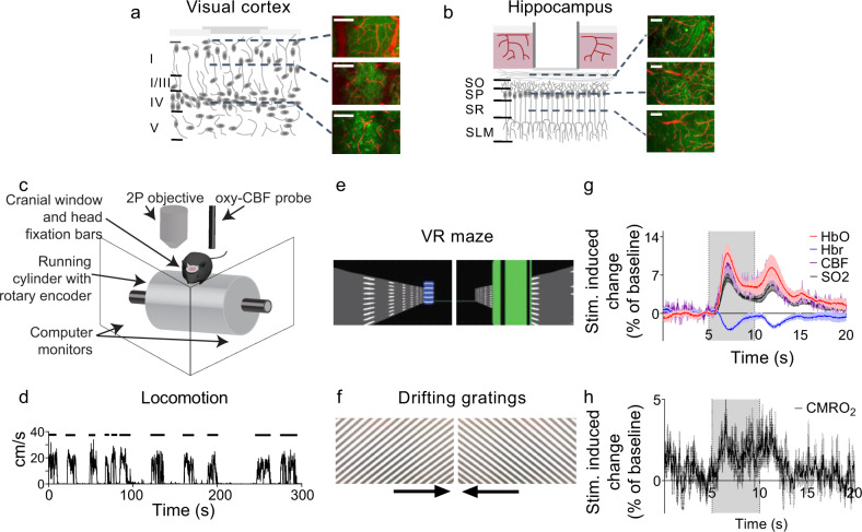
Fig. 1
Experimental set-up and example haemodynamic data.
Representative schematic showing the GCaMP6f-positive pyramidal neurons (green) and blood vessels (red) accessible for two-photon imaging after a visual cortical or b hippocampal surgery, with example...
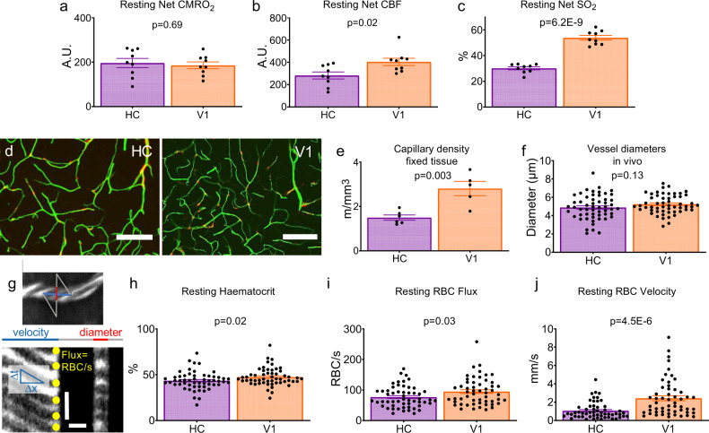
Fig. 2
Baseline haemodynamics in HC and V1.
Estimated CMRO 2 a , CBF b and oxygen saturation (SO 2 ) c in HC (purple) and V1 (orange) in stationary mice in the dark (HC: 9 animals across 21 sessions; V1: 9 animals across 19 sessions, 1u20135 se...
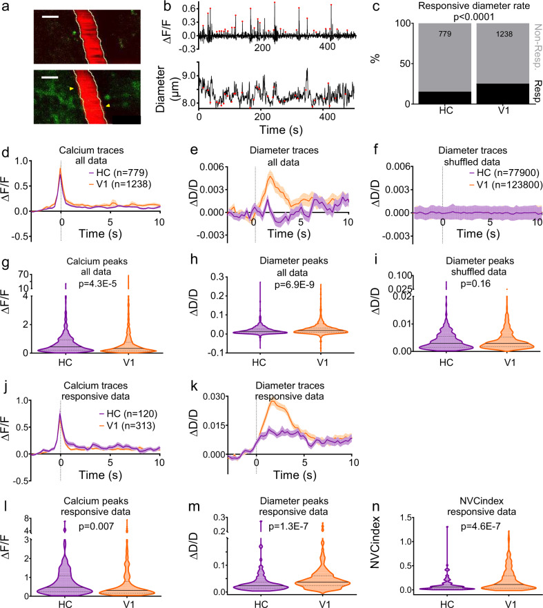
Fig. 3
Vessel responses to local neuronal calcium events.
a Texas Red dextran-filled vessel (red) and GCaMP6f-positive pyramidal neurons (green) from one recording in V1 before (top) and during (bottom) increases in neuronal calcium (to represent the 87 vess...
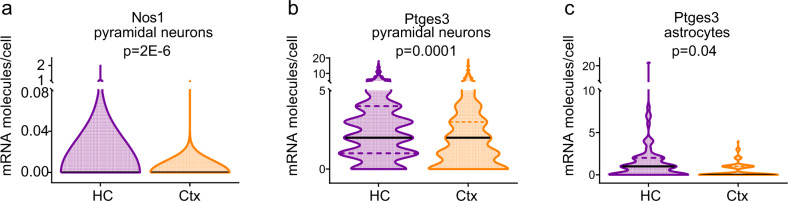
Fig. 4
Vasodilatory second messenger pathways in HC and cortex.
The expression of a Nos1 and b Ptges3 were higher in the pyramidal cells of HC (941 cells) than cortex (398 cells). c Ptges3 expression was also higher in astrocytes in HC (80 cells) than V1 (143 cell...
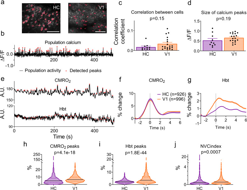
Fig. 5
Wide-field neuronal activity patterns.
a Representative wide field-of-view recording of calcium signals (white; maximum projection across time) in HC (left, 1 of 10 independent recordings) and V1 (right, 1 of 19 independent recordings). Re...
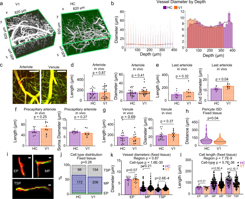
Fig. 6
Vascular morphology across brain regions.
a Example in vivo Z-stacks of vasculature in V1 (left) and HC (CA1, right, as used in b ). b Left panel: all data points for vessel diameters by depth from the pia in V1 (48458 vessels collapsed from ...
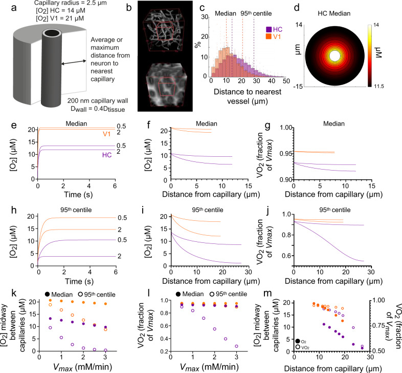
Fig. 7
Modelling O 2 diffusion in brain tissue.
a Schematic of radial diffusion model. b Top: example in vivo Z-stack (250u2009u03bcmu00b3) of fluorescent dextran-filled vasculature in CA1. Bottom: 3D distance map generated from the z-stack. White ...
Figure images are served from the NIH/NLM PubMed Central Open Access Subset or Europe PMC; copyright remains with the publishers and authors.
💬 Discussion
0 commentsNo comments yet. Be the first to start a discussion!
Leave a Comment