Abstract
AbstractSelf-assembled DNA nanostructures feature an unprecedented addressability with sub-nanometer precision and accuracy. This addressability relies on the ability to attach functional entities to single DNA strands in these structures. The efficiency of this attachment depends on two factors: incorporation of the strand of interest and accessibility of this strand for downstream modification. Here we use DNA-PAINT super-resolution microscopy to quantify both incorporation and accessibility of all individual strands in DNA origami with molecular resolution. We find that strand incorporation strongly correlates with the position in the structure, ranging from a minimum of 48% on the edges to a maximum of 95% in the center. Our method offers a direct feedback for the rational refinement of the design and assembly process of DNA nanostructures and provides a long sought-after quantitative explanation for efficiencies of DNA-based nanomachines.
🔬 Techniques
🔭 Microscopes
💻 Software
✨ Fluorophores
🏭 Microscope Brands
🧪 Reagent Suppliers
🔴 Lasers
📷 Detectors
🎨 Filters
💻 Software Details
🏛️ Research Organizations (ROR)
Affiliated research institutions:
📋 Methods
In silico validation of the method Transient, repetitive binding of dye-labeled oligonucleotides (“imager” strands) to their complementary targets (“docking” sites) can be observed as apparent blinking (Fig. 1a ). The apparent blinking is used to reconstruct super-resolution images that visualize the designed pattern of docking sites, e.g., a 20-nm-grid structure (based on the two-dimensional (2D) rectangular DNA origami, details about the design are shown in Supplementary Figs. 1 and 2 ). These 20-nm-grids, however, stochastically miss reconstructed points at designed sites 21 , 23 because the docking sites at these missing points are not transiently visited by an imager strand. This could be explained by two mechanisms: (1) staples are not incorporated into the structure; or (2) staples are incorporated, but docking sites are not available for binding of imager strands (i.e., sequestered). As a result, these positions are not accessible for downstream modification (Fig. 1b ). To assess this accessibility, we developed a software tool that detected DNA origami structures in a reconstructed DNA-PAINT image and subsequently aligned them to a template structure to create a sum image (Fig. 1c and Supplementary Figs. 3 and 4 ). Then, we quantified the number of localizations at each docking site in the sum image. As the binding of imager strands to their docking sites is repetitive, we defined a minimum number of localizations as a threshold value: sites with values below this threshold were classified as not detected (Fig. 1c ). To validate our analysis workflow, we performed in silico DNA-PAINT experiments of 20-nm-grids with an occurrence probability of individual docking sites ranging from 30 to 100% using the software program Picasso 21 . The number of detected docking sites was in good agreement with the number of simulated docking sites (Fig. 1d ), which confirmed the applicability of our analysis approach to measure the detectability of single docking sites. Fig. 1 Quantification of detected staples in DNA origami using super-resolution. a DNA-PAINT concept: transient hybridization of dye-labeled imager strands to docking sites on DNA origami enables super-resolution imaging. b Typical DNA-PAINT image of 20-nm-grids allows distinction of individual binding sites. Zoom-in of a 20-nm-grid shows that some of the 12 grid sites were not detected. c Quantification workflow for assessing abundance of docking sites. Single structures were selected and aligned to a template of the designed grid structure by image cross-correlation. Subsequently, a histogram of localizations per grid site was used to determine a cut-off threshold below, which a site is defined as not detected. This threshold is defined as the number of localizations at half-maximum as determined by the Gaussian fit (magenta curve). d Benchmarking of the detection workflow was performed using simulated ground-truth DNA-PAINT data. Blue dots represent simulated 20-nm-grids with varying percentage of simulated docking sites and their evaluation result. The dashed line is the identity line. Scale bars: 100 nm in b , 20 nm in d
Show full methods section
In silico validation of the method Transient, repetitive binding of dye-labeled oligonucleotides (“imager” strands) to their complementary targets (“docking” sites) can be observed as apparent blinking (Fig. 1a ). The apparent blinking is used to reconstruct super-resolution images that visualize the designed pattern of docking sites, e.g., a 20-nm-grid structure (based on the two-dimensional (2D) rectangular DNA origami, details about the design are shown in Supplementary Figs. 1 and 2 ). These 20-nm-grids, however, stochastically miss reconstructed points at designed sites 21 , 23 because the docking sites at these missing points are not transiently visited by an imager strand. This could be explained by two mechanisms: (1) staples are not incorporated into the structure; or (2) staples are incorporated, but docking sites are not available for binding of imager strands (i.e., sequestered). As a result, these positions are not accessible for downstream modification (Fig. 1b ). To assess this accessibility, we developed a software tool that detected DNA origami structures in a reconstructed DNA-PAINT image and subsequently aligned them to a template structure to create a sum image (Fig. 1c and Supplementary Figs. 3 and 4 ). Then, we quantified the number of localizations at each docking site in the sum image. As the binding of imager strands to their docking sites is repetitive, we defined a minimum number of localizations as a threshold value: sites with values below this threshold were classified as not detected (Fig. 1c ). To validate our analysis workflow, we performed in silico DNA-PAINT experiments of 20-nm-grids with an occurrence probability of individual docking sites ranging from 30 to 100% using the software program Picasso 21 . The number of detected docking sites was in good agreement with the number of simulated docking sites (Fig. 1d ), which confirmed the applicability of our analysis approach to measure the detectability of single docking sites. Fig. 1 Quantification of detected staples in DNA origami using super-resolution. a DNA-PAINT concept: transient hybridization of dye-labeled imager strands to docking sites on DNA origami enables super-resolution imaging. b Typical DNA-PAINT image of 20-nm-grids allows distinction of individual binding sites. Zoom-in of a 20-nm-grid shows that some of the 12 grid sites were not detected. c Quantification workflow for assessing abundance of docking sites. Single structures were selected and aligned to a template of the designed grid structure by image cross-correlation. Subsequently, a histogram of localizations per grid site was used to determine a cut-off threshold below, which a site is defined as not detected. This threshold is defined as the number of localizations at half-maximum as determined by the Gaussian fit (magenta curve). d Benchmarking of the detection workflow was performed using simulated ground-truth DNA-PAINT data. Blue dots represent simulated 20-nm-grids with varying percentage of simulated docking sites and their evaluation result. The dashed line is the identity line. Scale bars: 100 nm in b , 20 nm in d
Methods
Materials and buffers Unmodified, dye-labeled, and biotinylated DNA oligonucleotides were purchased from MWG Eurofins or Integrated DNA Technologies. DNA scaffold strands were purchased from Tilibit (p7249, identical to M13mp18). Streptavidin was purchased from Thermo Fisher (catalog number: S-888). Bovine serum albumin (BSA) and BSA-biotin obtained from Sigma-Aldrich (catalog number: A8549). Glass slides and coverslips were purchased from Marienfeld (cat. no. 0107032) and Thermo Fisher (cat. No. 10756991). Freeze ‘N Squeeze columns were ordered from Bio-Rad (cat. no. 732-6165). Polyethylene glycol (PEG)-8000 was purchased from Merck (cat. No. 6510-1KG). Four buffers were used for sample preparation and imaging: buffer A (10 mM Tris-HCl pH 7.5, 100 mM NaCl, 0.05% Tween 20, pH 7.5); buffer B (5 mM Tris-HCl pH 8, 10 mM MgCl 2 , 1 mM EDTA, 0.05% Tween 20, pH 8); buffer O (5 mM Tris-HCl pH 8, 12.5 mM MgCl 2 , 1 mM EDTA, 0.05% Tween 20, pH 8) and buffer O + (same as O, but supplemented with 1× PCA, 1× PCD, and 1× Trolox). A concentration of 100× Trolox: 100 mg Trolox, 430 μl 100% Methanol, 345 μl 1 M NaOH in 3.2 ml H 2 O. A concentration of 40× PCA: 154 mg PCA, 10 ml water, and NaOH were mixed and adjusted to pH 9.0. 100× PCD: 9.3 mg PCD, 13.3 ml of buffer (100 mM Tris-HCl pH 8, 50 mM KCl, 1 mM EDTA, 50% Glycerol). PEG-buffer was used for PEG precipitation 37 (15% PEG-8000, 500 mM NaCl, 12.5 mM MgCl 2 in TAE pH 8.0).
Super-resolution microscopy setup
Fluorescence imaging was carried out on an inverted Nikon Eclipse Ti microscope (Nikon Instruments) with the Perfect Focus System, applying an objective-type total internal reflection fluorescence (TIRF) configuration with an oil-immersion objective (Apo SR TIRF 100×, NA 1.49, Oil). Two lasers were used for excitation: 561 nm (200 mW, Coherent Sapphire) or 640 nm (150 mW, Toptica iBeam smart). The laser beam was passed through cleanup filters (ZET561/10 or ZET642/20, Chroma Technology) and coupled into the microscope objective using a beam splitter (ZT561rdc or ZT647rdc, Chroma Technology). Fluorescence light was spectrally filtered with an emission filter (ET600/50m and ET575lp or ET705/72m and ET665lp, Chroma Technology) and imaged on an electron-multiplying charge-coupled device (EMCCD) camera (Andor iXon Ultra 897, used for Figs. 1a and 3c ) or sCMOS camera (Andor Zyla 4.2, used for Figs. 3b , d, and 4 ) without further magnification, resulting in an effective pixel size of 160 nm (EMCCD) or 130 nm (sCMOS after 2 × 2 binning).
DNA origami self-assembly
Self-assembly of DNA origami was accomplished in a one-pot reaction mix with 40 µl total volume, consisting of 10 nM scaffold strand, 100 nM folding staples, 10 nM biotinylated staples (500 nM for Fig. 2 and Supplementary Fig. 16d ), and 1 µM (Figs. 1 b, 2 , 3b, and 4 ) or varying concentrations (Fig. 3c ) of docking site strands (5′-staple-TTATACATCTA-3′) in folding buffer (1× TE buffer with 12.5 mM MgCl 2 ). The reaction mix was then subjected to a thermal annealing ramp using a thermocycler (Mastercycler Nexus Gradient, Eppendorf or Tetrad 2, Bio-Rad). If not otherwise noted, the reaction mix was first incubated at 80 °C for 5 min and then cooled from 60 to 4 °C in steps of 1 °C per 3.21 min and then held at 4 °C until stored at −20 °C protected from light. Samples for the measurement with varying staple excess (Fig. 3c ) were purified via three rounds of PEG precipitation by adding the same volume of PEG-buffer, centrifuging at 10,000× g at 4 °C for 30 min, removing the supernatant, and resuspending in folding buffer. Structures for Fig. 2 were gel purified by mixing with 1× loading dye and subsequently subjected to agarose gel electrophoresis (1.5% agarose, 0.5× TAE, 10 mM MgCl 2 , 1× SYBR Safe) at 3 V cm −1 for 3 h. Gel bands were extracted, crushed, filled into a Freeze ‘N Squeeze column, and centrifuged for 5 min at 1000× g at 4 °C. Force-clamp structures were designed and assembled as described before 27 . The staple excess of the extended staple in the structure of Supplementary Fig. 16d was 100× over the scaffold.
Sample preparation
For sample preparation, a piece of coverslip and a glass slide were sandwiched together by two strips of double-sided tape (Scotch, cat. no. 665D) to form a flow chamber with inner volume of ~20 μl. First, 20 µl of biotin-labeled bovine albumin (1 mg/ml, dissolved in buffer A) was flushed into the chamber and incubated for 2 min. The chamber was then washed with 40 µl of buffer A. A volume of 20 µl of streptavidin (0.5 mg ml −1 , dissolved in buffer A) was then flushed through the chamber and allowed to bind for 2 min. After washing with 20 µl of buffer A and subsequently with 20 µl of buffer B, 20 µl of biotin-labeled DNA structures (~100–400 pM, see Supplementary Table 4 ) in buffer B were flushed into the chamber and incubated for 2 min. The chamber was washed with 40 µl of buffer B. Finally, 20 µl of the imager solution was flushed into the chamber, which was subsequently sealed with epoxy (Toolcraft, cat. no. TC-EPO5-24) before imaging.
Imaging conditions
Refer to Supplementary Table 4 for an overview of imaging conditions and Supplementary Table 5 for the imager strand sequences. Supplementary Table 3 shows the super-resolution data properties of all measurements.
Data simulation
In silico experiments were performed using the simulation module of the Picasso 18 software package. For Fig. 1c , 50 structures consisting of 12 BS spaced 20 nm apart (the “20-nm-grid” structure) were simulated with varying incorporation of staple strands (30–100%). Further simulation parameters were an image size of 128 × 128 px and an acquisition time of 50 min (15,000 frames at 200 ms integration time). For the simulation of the 3 BS and 6 BS structure of Fig. 3d , again 50 structures with the same parameters were simulated. For each simulation run, a dark time of 12.5 s and a bright time of 0.5 s were used, corresponding to 5 nM imager strand concentration at a constant association rate of 1.6 × 10 6 M −1 s −1 . Further simulation parameters were a pixel size of 160 nm, a detection rate of 35 photons × ms −1 kW −1 cm −2 , a budget of 1.5 × 10 6 photons, a power density of 1.5 kW × cm −2 , and a full width half-maximum of the point-spread-function of 309 nm.
Data analysis
First, super-resolution images were reconstructed and drift-corrected with the render module of Picasso. For the automated evaluation with our MATLAB program, individual structures were selected with Picasso’s “pick similar” feature. For the experiments involving the detection of single BS (Figs. 3d and 4 ), structures were additionally filtered manually by using Picasso’s “plot pick” feature. Structures that did not display a correct alignment pattern were discarded. An overview of all selected structures is shown in Supplementary Figs. 9 , 10 , 12 , and 13 . Localizations of selected structures were saved as *.hdf5 file and subsequently converted to a *.trace.mat, drift file and mbox file, which then could be imported into the MATLAB program. The template of each structure was automatically generated after selection of the docking site pattern on the 2D origami map in the template tool. An image was generated by placing Gaussian distributions ( σ = 3 nm, σ = 2 nm for Fig. 3c or σ = 1 nm for the single site measurements shown in Figs. 3d and 4 ) of binding events on the previously defined positions. For evaluation, a subset with n structures of all selected structures in the *.trace.mat file was used (Fig. 3b, c : n = 500; Fig. 3d : n = 250; Fig. 4 : two datasets were combined and the minimum number of structures that was present for each structure type was used, n = 186). Next, the software aligned each structure to the structure template: the localizations of each structure were isolated and a super-resolution image of the structure was generated by calculating a 2D histogram of these localizations. The super-resolution image was rotated stepwise in a circle and in each step cross-correlated to the template image. The rotation angle with the highest correlation coefficient was determined. This rotation angle and the corresponding xy -shift were then used to transform the localization list in order to align the structure to its template. After alignment, the program counted the number of localizations in a circle with a diameter of 20 nm (Figs. 1c and 3c ), 18 nm (Fig. 3b ), 6 nm (Fig. 4 ), or 5 nm (Fig. 3d ) around the predefined docking site positions of the template. The number of localizations per docking site for all structures was displayed in a histogram within the program. This histogram was used to determine the correct detection threshold. This threshold was subsequently used to calculate the presence of each docking site for a given structure. Finally, the program displayed the percentage of detected docking sites for all evaluated structures. For dual-channel measurements (Fig. 2 ), 100 structures were manually selected in the reconstructed super-resolution image from Picasso. For each selected structure, the presence or absence of both colors at each docking site was registered.
Data availability
All data supporting the findings of this study are available within the paper and its Supplementary Information. All RAW data are available upon request. The MATLAB program and source code for evaluation are available for download at http://www.jungmannlab.org . All sequences of the DNA origami structures are given in Supplementary Tables 6 and 7 .
Materials and buffers Unmodified, dye-labeled, and biotinylated DNA oligonucleotides were purchased from MWG Eurofins or Integrated DNA Technologies. DNA scaffold strands were purchased from Tilibit (p7249, identical to M13mp18). Streptavidin was purchased from Thermo Fisher (catalog number: S-888). Bovine serum albumin (BSA) and BSA-biotin obtained from Sigma-Aldrich (catalog number: A8549). Glass slides and coverslips were purchased from Marienfeld (cat. no. 0107032) and Thermo Fisher (cat. No. 10756991). Freeze ‘N Squeeze columns were ordered from Bio-Rad (cat. no. 732-6165). Polyethylene glycol (PEG)-8000 was purchased from Merck (cat. No. 6510-1KG). Four buffers were used for sample preparation and imaging: buffer A (10 mM Tris-HCl pH 7.5, 100 mM NaCl, 0.05% Tween 20, pH 7.5); buffer B (5 mM Tris-HCl pH 8, 10 mM MgCl 2 , 1 mM EDTA, 0.05% Tween 20, pH 8); buffer O (5 mM Tris-HCl pH 8, 12.5 mM MgCl 2 , 1 mM EDTA, 0.05% Tween 20, pH 8) and buffer O + (same as O, but supplemented with 1× PCA, 1× PCD, and 1× Trolox). A concentration of 100× Trolox: 100 mg Trolox, 430 μl 100% Methanol, 345 μl 1 M NaOH in 3.2 ml H 2 O. A concentration of 40× PCA: 154 mg PCA, 10 ml water, and NaOH were mixed and adjusted to pH 9.0. 100× PCD: 9.3 mg PCD, 13.3 ml of buffer (100 mM Tris-HCl pH 8, 50 mM KCl, 1 mM EDTA, 50% Glycerol). PEG-buffer was used for PEG precipitation 37 (15% PEG-8000, 500 mM NaCl, 12.5 mM MgCl 2 in TAE pH 8.0).
Electronic supplementary material Supplementary Information Peer Review File
📊 Figures
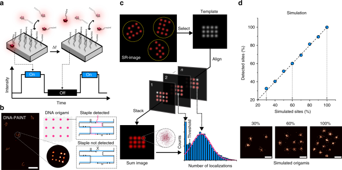
Fig. 1
Quantification of detected staples in DNA origami using super-resolution. a DNA-PAINT concept: transient hybridization of dye-labeled imager strands to docking sites on DNA origami enables super-resol...
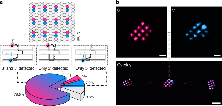
Fig. 2
Experimental validation of accessibility and incorporation efficiency. a The 20-nm-grid staples were extended with orthogonal DNA-PAINT docking sites on the 3u2032-end (magenta) and 5u2032-end (blue) ...
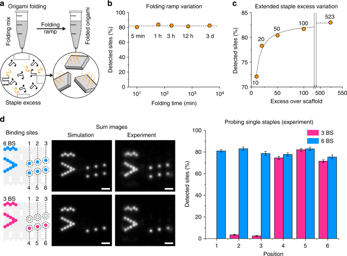
Fig. 3
Influence of folding conditions and experimental validation of accessibility of single sites. a Schematic folding of 20-nm-grids with the staples that carry detection sites in orange. b Percentage of ...
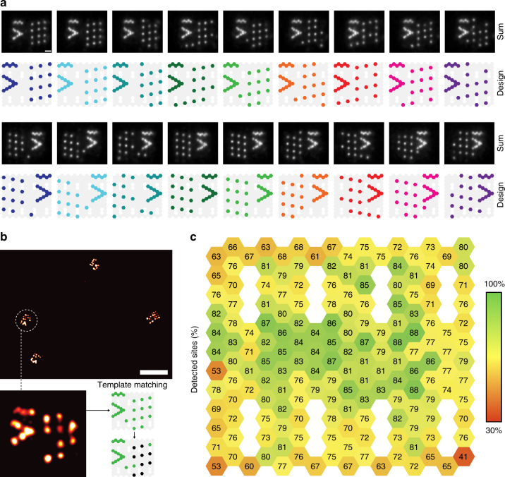
Fig. 4
Accessibility of all staples in a 2D rectangle. a A total of 18 design variants were used to probe all addressable staples in a 2D rectangular DNA origami structure in a single experiment. Designed pa...
Figure images are served from the NIH/NLM PubMed Central Open Access Subset or Europe PMC; copyright remains with the publishers and authors.
💬 Discussion
0 commentsNo comments yet. Be the first to start a discussion!
Leave a Comment