Abstract
1300 nm three-photon calcium imaging has emerged as a useful technique to allow calcium imaging in deep brain regions. Application to large-scale neural activity imaging entails a careful balance between recording fidelity and perturbation to the sample. We calculated and experimentally verified the excitation pulse energy to achieve the minimum photon count required for the detection of calcium transients in GCaMP6s-expressing neurons for 920 nm two-photon and 1320 nm three-photon excitation. By considering the combined effects of in-focus signal attenuation and out-of-focus background generation, we quantified the cross-over depth beyond which three-photon microscopy outpeforms two-photon microscopy in recording fidelity. Brain tissue heating by continuous three-photon imaging was simulated with Monte Carlo method and experimentally validated with immunohistochemistry. Increased immunoreactivity was observed with 150 mW excitation power at 1 and 1.2 mm imaging depths. Our analysis presents a translatable model for the optimization of three-photon calcium imaging based on experimentally tractable parameters.
🔬 Techniques
🧬 Organisms
✨ Fluorophores
🧪 Sample Preparation
🏭 Microscope Brands
🧪 Reagent Suppliers
🔴 Lasers
📷 Detectors
💻 Software Details
💾 Data Repositories
🏷️ Research Resource Identifiers (RRIDs)
Verified research resources used in this paper:
🏛️ Research Organizations (ROR)
Affiliated research institutions:
📋 Methods
Key resources table
Reagent type (species) or resource Designation Source or reference Identifiers Additional information Strain, strain background ( Mus musculus ) B6.Cg-Tg(CamK2a-tTA)1Mmay/J The Jackson Laborartory Stock: 007004 MGI:2179066 Strain, strain background ( Mus musculus ) B6;DBA-Tg(tetO-GCaMP6s)2Niell/J The Jackson Laborartory Stock: 024742 MGI:5553332 Antibody anti-HSP70/72 (mouse monoclonal) Enzo Life Sciences, Cat# SPA-810PED RRID: AB-2264369 IHC(1:400) Antibody anti-GFAP (mouse monoclonal) Sigma-Aldrich, Cat# G3893 RRID: AB_477010 IHC(1:760) Antibody anti-Iba1 (mouse monoclonal) Sigma-Aldrich, Cat# SAB2702364 RRID: AB_2820253 IHC(1:1000) Antibody Goat anti-mouse (polyclonal) Thermo Fisher Scientific, Cat# A-11003 RRID: AB_2534071 IHC(1:500) Software, algorithm Source code 1 : matlab code for simulating the brain temperature distribution under continuous long-wavelength illumination by 3PM using Monte Carlo method and heat equation. Mathworks, Matlab 2016b RRID: SCR_001622 Simultaneous 1320 nm 3PM and 920 nm 2PM Imaging with Time Division Multiplex Scheme The excitation source for 1320 nm 3PM was a noncollinear optical parametric amplifier (NOPA, Spectra-Physics) pumped by an ultrafast amplifier (Spirit, Spectra-Physics). The excitation source for 920 nm 2PM was a mode-locked Ti:Sapphire laser (Tsunami, Spectra-Physics). The two excitation beams were launched into a custom-built microscope, described in our previous works ( Ouzounov et al., 2019 ; Ouzounov et al., 2017 ). The 3PE wavelength was centered at 1320 nm and 2PE at 920 nm for the optimal d ′ ( Ouzounov et al., 2019 ). The two excitation beams were verified to have similar spatial resolution well below the size of neurons or blood vessels such that their excitation volumes are almost identical ( Ouzounov et al., 2019 ). Time-division multiplex (TDM) achieves nearly simultaneous 2PM and 3PM imaging by alternating between spatially overlapped 920 nm and 1320 nm laser beams on a microsecond time scale. 2PE and 3PE fluorescence signals were separated according to the recorded laser clock. More details about the setup can be found in Ouzounov et al. (2017) . The calcium activities were recorded with 13.6 Hz frame rate, limited by the fastest achievable line rate of the galvanometer scanners. This frame rate is sufficiently high for imaging the temporal dynamics of GCaMP6s ( τ 1 / e ~ 2 s). For 2PM and 3PM comparison experiments, the FOV was reduced to fit a single neuron so that the signal-to-noise ratio was maximized to ensure accurate comparison between 2PM and 3PM calcium traces. The excitation power for 3PM and 2PM was adjusted to generate similar photon count per frame that lead to the same noise level, and the FOV was reduced to increase the laser dwell time on neuron bodies. Photon counting schemes The microscope was first tested for shot-noise limited performance by photon counting the signal generated by stationary 1320-nm or 920-nm beam focused in fluorescein solution (~40 μM and pH=10). The laser power was chosen (~0.3 mW for both wavelengths) to ensure the photon counts per second is lower than 5% of the laser repetition rate of the NOPA, which limits the photon stacking error to within 2.5% of the total counts. According to Poisson statistics, photon stacking error causes a fraction of 1 - ( 1 - e - λ ) / λ underestimation in photon counts, where λ is the average count per second divided by the laser repetition rate. For 2PE using the Ti:Sapphire laser, the photon stacking error is negligible since the typical photon counts are below 1% of its repetition rate (80 MHz). In this experiment, the PMT (Hamamatsu H7422-40) anode current was first amplified with a 10 MHz bandwidth pre-amplifier (C9999, Hamamatsu), and then counted by a photon counter (SR400, Stanford Research). Shot-noise limited performance was confirmed for our imaging system. During imaging, the photon counts of neurons were obtained by converting pixel values to photon counts according to a conversion factor. The calibration was done by parking a 920 nm or 1320 nm focus in a fluorescein solution sample and then perform photon counting and imaging consecutively. Linearity between pixel values and photon counts was tested by changing the laser power, and the ratio between them was used as the conversion factor. In fact, recording analog value is a better way to measure high photon counts, since there is no photon stacking error and the voltage signal can simply be summed. The conversion factor was further confirmed by observing the first mode in a pixel value histogram. The zeroth mode of a pixel histogram peaks at PMT offset value, and the first mode is larger than that, representing pixels receiving exactly one photon. Higher-order modes can also be observed, representing pixels receiving multiple photons. For all simultaneous 2P and 3P imaging, the sampling frequency was 5 MHz, so that direct photon counting based on images could also be performed, which showed consistent results in comparison to analog recordings. Measurement of excitation light attenuation in the brain tissue based on fluorescence signal The vasculature imaging was performed simultaneously with 2PM and 3PM using the TDM scheme. The image stack was taken with 10 μm step size in depth, and the imaging power was increased with imaging depth to keep the signal level approximately constant. The signal of each frame was calculated as the average of the brightest 0.5% pixel values and then converted to photon counts per excitation pulse according to the method described in the previous section. The fraction of excitation power reaching the focus from the brain surface (Focus Power/Surface Power) was calculated as the square (cubic) root of the ratio of the 2PE (3PE) signal at the imaging depth and at the brain surface.
Show full methods section
Key resources table
Reagent type (species) or resource Designation Source or reference Identifiers Additional information Strain, strain background ( Mus musculus ) B6.Cg-Tg(CamK2a-tTA)1Mmay/J The Jackson Laborartory Stock: 007004 MGI:2179066 Strain, strain background ( Mus musculus ) B6;DBA-Tg(tetO-GCaMP6s)2Niell/J The Jackson Laborartory Stock: 024742 MGI:5553332 Antibody anti-HSP70/72 (mouse monoclonal) Enzo Life Sciences, Cat# SPA-810PED RRID: AB-2264369 IHC(1:400) Antibody anti-GFAP (mouse monoclonal) Sigma-Aldrich, Cat# G3893 RRID: AB_477010 IHC(1:760) Antibody anti-Iba1 (mouse monoclonal) Sigma-Aldrich, Cat# SAB2702364 RRID: AB_2820253 IHC(1:1000) Antibody Goat anti-mouse (polyclonal) Thermo Fisher Scientific, Cat# A-11003 RRID: AB_2534071 IHC(1:500) Software, algorithm Source code 1 : matlab code for simulating the brain temperature distribution under continuous long-wavelength illumination by 3PM using Monte Carlo method and heat equation. Mathworks, Matlab 2016b RRID: SCR_001622 Simultaneous 1320 nm 3PM and 920 nm 2PM Imaging with Time Division Multiplex Scheme The excitation source for 1320 nm 3PM was a noncollinear optical parametric amplifier (NOPA, Spectra-Physics) pumped by an ultrafast amplifier (Spirit, Spectra-Physics). The excitation source for 920 nm 2PM was a mode-locked Ti:Sapphire laser (Tsunami, Spectra-Physics). The two excitation beams were launched into a custom-built microscope, described in our previous works ( Ouzounov et al., 2019 ; Ouzounov et al., 2017 ). The 3PE wavelength was centered at 1320 nm and 2PE at 920 nm for the optimal d ′ ( Ouzounov et al., 2019 ). The two excitation beams were verified to have similar spatial resolution well below the size of neurons or blood vessels such that their excitation volumes are almost identical ( Ouzounov et al., 2019 ). Time-division multiplex (TDM) achieves nearly simultaneous 2PM and 3PM imaging by alternating between spatially overlapped 920 nm and 1320 nm laser beams on a microsecond time scale. 2PE and 3PE fluorescence signals were separated according to the recorded laser clock. More details about the setup can be found in Ouzounov et al. (2017) . The calcium activities were recorded with 13.6 Hz frame rate, limited by the fastest achievable line rate of the galvanometer scanners. This frame rate is sufficiently high for imaging the temporal dynamics of GCaMP6s ( τ 1 / e ~ 2 s). For 2PM and 3PM comparison experiments, the FOV was reduced to fit a single neuron so that the signal-to-noise ratio was maximized to ensure accurate comparison between 2PM and 3PM calcium traces. The excitation power for 3PM and 2PM was adjusted to generate similar photon count per frame that lead to the same noise level, and the FOV was reduced to increase the laser dwell time on neuron bodies. Photon counting schemes The microscope was first tested for shot-noise limited performance by photon counting the signal generated by stationary 1320-nm or 920-nm beam focused in fluorescein solution (~40 μM and pH=10). The laser power was chosen (~0.3 mW for both wavelengths) to ensure the photon counts per second is lower than 5% of the laser repetition rate of the NOPA, which limits the photon stacking error to within 2.5% of the total counts. According to Poisson statistics, photon stacking error causes a fraction of 1 - ( 1 - e - λ ) / λ underestimation in photon counts, where λ is the average count per second divided by the laser repetition rate. For 2PE using the Ti:Sapphire laser, the photon stacking error is negligible since the typical photon counts are below 1% of its repetition rate (80 MHz). In this experiment, the PMT (Hamamatsu H7422-40) anode current was first amplified with a 10 MHz bandwidth pre-amplifier (C9999, Hamamatsu), and then counted by a photon counter (SR400, Stanford Research). Shot-noise limited performance was confirmed for our imaging system. During imaging, the photon counts of neurons were obtained by converting pixel values to photon counts according to a conversion factor. The calibration was done by parking a 920 nm or 1320 nm focus in a fluorescein solution sample and then perform photon counting and imaging consecutively. Linearity between pixel values and photon counts was tested by changing the laser power, and the ratio between them was used as the conversion factor. In fact, recording analog value is a better way to measure high photon counts, since there is no photon stacking error and the voltage signal can simply be summed. The conversion factor was further confirmed by observing the first mode in a pixel value histogram. The zeroth mode of a pixel histogram peaks at PMT offset value, and the first mode is larger than that, representing pixels receiving exactly one photon. Higher-order modes can also be observed, representing pixels receiving multiple photons. For all simultaneous 2P and 3P imaging, the sampling frequency was 5 MHz, so that direct photon counting based on images could also be performed, which showed consistent results in comparison to analog recordings. Measurement of excitation light attenuation in the brain tissue based on fluorescence signal The vasculature imaging was performed simultaneously with 2PM and 3PM using the TDM scheme. The image stack was taken with 10 μm step size in depth, and the imaging power was increased with imaging depth to keep the signal level approximately constant. The signal of each frame was calculated as the average of the brightest 0.5% pixel values and then converted to photon counts per excitation pulse according to the method described in the previous section. The fraction of excitation power reaching the focus from the brain surface (Focus Power/Surface Power) was calculated as the square (cubic) root of the ratio of the 2PE (3PE) signal at the imaging depth and at the brain surface.
Measurement of the pulse energy required per 0.1 photon detection
To have a fair comparison on the excitation efficiency of 920 nm 2PM and 1320 nm 3PM, we controlled all the parameters regarding 2PE and 3PE except for the wavelength. For both wavelengths, the axial resolution was made equal by adjusting the beam size at the back aperture of the objective separately. The point spread functions of both wavelengths were also overlapped laterally (by fine-tuning the 920 nm beam pointing direction) and axially (by changing the field curvature of the 920 nm beam at the objective lens back aperture by fineadjustment of the distance between the lenses of a 1:1 telescope). For both wavelengths, the pulse durations were scaled to 60 fs (measured pulse durations were 60–70 fs in FWHM for 1320 nm, and 180–200 fs for 920 nm. All pulses were assumed to have sech 2 profile). Light absorption by the immersion water was taken into account when calculating the pulse energy for 1320 nm on the brain surface. As we show in Figure 3—figure supplement 1 , it is important to distinguish the pulse energy on the brain surface and after the objective lens for 1320 nm excitation. Based on the fluorescence signals derived from simultaneous 2P and 3P imaging, Figure 1B was plotted using the following equations ( Xu and Webb, 1997 ): (3) S 2 P / f = C 2 ( P / f ) 2 / τ (4) S 3 P / f = C 3 P / f 3 / τ 2 where S n P / f is the n-photon-excited signal yield in the unit of detected photon/pulse, P is the average power at the brain surface, f is the repetition rate, τ is the pulse duration, and C n (n=2 and 3) are the coefficients to be determined. For vasculature imaging, S n P / f is calculated as the average of the brightest 0.5% pixel values per frame, converted to photon counts. For GCaMP6s-labeled neurons, S n P / f was calculated from the sum of time-averaged pixel values in cell bodies (averaging time = 75 s, on 37 different cells in 5 animals). Given that P / f and τ are already measured during the experiment, C n can be solved. To produce Figure 1B , we plugged C n into the equations and set the signal yield (i.e., S n P / f ) to 0.1 photon per pulse, pulse duration to 60 fs, and then solve for pulse energy P / f on the sample surface according to Equations 3 and 4 . To account for the EAL variation recorded from different animals in Figure 1B , we measured EAL of the cortical layers of each animal by imaging fluorescein-labeled blood vessels immediately after calcium imaging. The depths of neurons were rescaled by dividing the measured EAL and then multiplying with the nominal EAL (i.e., 293 μm for 1320 nm 3PE and 154 μm for 920 nm, as measured by the vasculature data). The logarithm of the neuron signal was plotted against depth, and then fitted with a linear model for the slope and intercept ( Figure 1B ). The slope equals l n ( 10 ) / E A L , and the intercept equals to the pulse energy required to yield 0.1 detected photon per pulse on the sample surface (i.e., zero imaging depth).
Measurement of Signal-to-background ratio
The signal of each frame was measured as the average of the brightest 0.1% pixel values. For vasculature data, the background was measured as the average pixel values of regions surrounding the blood vessels (i.e., not labeled). For GCaMP6 neural data, the background was measured as the pixel value in the shadow of big blood vessels. The pixel values of cortical tissue surrounding the neurons cannot be used as background since it contains densely labeled neuronal processes except for area within the blood vessels. SBR was calculated as the signal divided by the background. Quantification of vasculature volume fraction and staining inhomogeneity The SBR limit of 2PM depends on the spatial inhomogeneity of staining ( Theer and Denk, 2006 ). We quantified the staining inhomogeneity of fluorescein-labeled vasculature in order to compare the in vivo SBR measurement to the theory and ex vivo fluorescent bead measurement ( Theer and Denk, 2006 ). The volume fraction of the vasculature can be estimated by the fraction of the stained blood vessel area in each xy image frame. Figure 2—figure supplement 1 shows the fractional vascular area vs. imaging depth, derived from the same 3PM dataset, as in Figure 2B . The segmentation of blood vessel regions was performed with graythresh function in MATLAB and then inspected manually for correctness. We concluded that the labeled vascular volume accounts for 2 ± 1% (mean ± standard deviation) in the imaged column of the mouse cortex (~2mm lateral and 2mm caudal to the Bregma point, Figure 2B ). Our result is in close agreement with other studies quantifying the fractional vascular volume by imaging sliced brains ex vivo (~2% for blood vessels of 20 μm or less diameter in the primary somatosensory cortex) ( Wang et al., 2019 ; Xiong et al., 2017 ). We noticed that most of the blood vessels in the imaged volume has a diameter of less than 20 μm, except for a few on the brain surface ( Figure 2—figure supplement 1A ). The blood vessel density is lower in the white matter (~750-850 μm) than that in the cortex ( Figure 2—figure supplement 1B ). The staining inhomogeneity is defined as, χ = C ^ / ⟨ C ⟩ , where C = C ( x , y , z ) denotes the spatial distribution of dye concentration in the entire imaged volume, C ^ is the maximum concentration, and C is the average concentration ( Theer and Denk, 2006 ). Staining inhomogeneity can be estimated as 1/(factional vascular volume) with the assumption that all the labeled blood vessels are equally bright ( C = 1 for all vasculature), and the rest of tissue is completely unstained ( C = 0 for the rest). Our experiments show that 2PM reaches SBR of 1 at about 4.7 EALs, that is 730 μm with EAL=154 μm ( Figure 2B ). This result is in close agreement to the 4.7 EALs predicted by theoretical calculation with a staining inhomogeneity of 50 ( Theer and Denk, 2006 ).
Analysis of the calcium traces of neurons
Sample motion in the original images, if any, was corrected by TurboReg plug-in in ImageJ. Regions of interest (ROIs) were generated by manual segmentation of neuron bodies. The pixel values of ROIs were exported to MATLAB 2016b for further processing. All the pixels in the ROI were summed and converted to photon counts. Spikes were inferred by thresholding the Poisson-distribution-based likelihood function derived from each trace ( Wilt et al., 2013 ). The discrimination threshold (denoted by C in the cited paper) was chosen to be l n ( ( 1 - r ) / r ) , where r is the estimated firing rate, which was estimated for each individual trace as the fraction of the trace that is more than 1.5 standard deviation above its mean. The baseline ( F 0 ) was determined by averaging trace values, after excluding the spikes and their rising and falling edges. For the processed traces in Figure 1C , fluorescence intensity traces were low-pass filtered with a hamming window of a time constant of 0.37 s. Traces ( F ) were normalized according to the equation ( F - F 0 ) / F 0 . Measurement of Δ F / F ratio from Simultaneously Recorded 3PM and 2PM Calcium Traces Based on the low-pass-filtered and normalized calcium traces described in the section above, the peaks of spikes were detected by finding local maxima that are larger than 30% Δ F / F in 3PM traces and have corresponding spike peaks detectable in 2PM traces. To produce the plot of Figure 2D , the ratios of 2PM and 3PM Δ F / F , that is Δ F / F 2 P / Δ F / F 3 P , of the same calcium transients were taken, and the depth of each neuron was normalized with the EAL of each animal. Monte Carlo simulation of light propagation and validation of tissue optical parameters We used Monte Carlo simulation to calculate light propagation in the brain tissue, following the algorithm described previously ( Stujenske et al., 2015 ). Podgorski et al. adapted the same numerical recipe to predict tissue temperature change during 2-photon imaging, which agreed well with experimental measurements at the wavelengths of 800 nm, 920 nm, and 1064 nm ( Podgorski and Ranganathan, 2016 ). In order to simulate for 1320 nm and 1280 nm excitation, we measured and estimated brain optical parameters as follows: For excitation wavelength longer than 1200 nm, water accounts for the majority of the light absorption in brain tissue in vivo ( Jacques, 2013 ). Therefore, tissue absorption coefficients μ a was approximated with 75% of the spectrum-weighted water absorption coefficient (defined in Section Measurement of Optical Absorption by Immersion Water), and the 75% is based on the water content of brain tissue ( Jacques, 2013 ; Tschöp et al., 2012 ). Tissue scattering coefficients μ s were then calculated from our measured effective attenuation lengths according to E A L = 1 / ( μ a + μ s ) , with EAL = 150 μm at 920 nm, and 300 μm at 1320 nm and 1280 nm. As cross-validation, the calculated scattering coefficient at 1320 nm is close to that measured by Gebhart et al. (i.e., 3.0 mm −1 ) ( Gebhart et al., 2006 ). We assumed an anisotropy factor g = 0.9 and tissue refractive index n = 1.36 for 920 nm, 1280 nm, and 1320 nm, since their variation in the wavelength range of interest is negligible. All the tissue optical parameters are summarized in Table 1 . To simulate underfilling of the objective back aperture, we initialized random photon distribution incident to the brain surface according to the relations: (5) w = w 0 − 1 / 2 l n ( X ) θ = s i n − 1 ( w / n 0 f ) r = t a n ( θ ) z where X is a random variable drawn from a uniform distribution from 0 to 1, w 0 is the 1/e 2 beam radius of the Gaussian beam at the objective back aperture, w is the radial distance to the objective optical axis of a randomly generated photon conforming to the Gaussian beam profile mentioned above, f is the objective focal length, n 0 is the refractive index of immersion water, z is the imaging depth in the sample. r and θ define, respectively, the radial coordinate of photon position and the polar angle of propagation direction, both with respect to the objective optical axis ( Figure 3—figure supplement 2 ). The objective (Olympus XLPLN25XWMP2, 25X, NA=1.05, focal length=7.2 mm) is under-filled, with 70% of its back aperture matched to the 1/e 2 beam diameter of a Gaussian beam, which gives an effective NA of ~ 0.75 ( Theer and Denk, 2006 ). The geometry of the simulation volume and boundary conditions are shown in Figure 3—figure supplement 2 . Heat diffusion model with Bio-heat equation Using the light intensity as the heat source, we calculated the temperature distribution by solving numerically the bio-heat Equation (6) , identical to that used previously by Stujenske et al. (2015) : (6) ρ c ∂ T ( r → , t ) ∂ t = k ∇ 2 T ( r → , t ) + ρ b c b w b ( T A − T ( r → , t ) ) + S h ( r → ) + q m where T r ⃑ , t is the spatial-temporal temperature distribution, S h r ⃑ is the radiative heat generation from Monto Carlo simulation, and the rest of the parameters and their values are listed in Table 3 , which are the same as in Stujenske et al. (2015) . Table 3. Thermal and mechanical properties of gray matter ( Stujenske et al., 2015 ). Variable Parameter Value Units ρ Density 1.04 × 10 −3 g/mm 3 c Brain specific heat 3.65 × 10 3 mJ/g°C k Thermal conductivity 0.527 mW/mm °C ρ b Blood density 1.06 × 10 −3 g/mm 3 c b Blood specific heat 3.6 × 10 3 mJ/g°C w b Blood perfusion rate 8.5 × 10 −3 /s q Metabolic heat 9.5 × 10 −3 mW/mm 3 T A Arterial temperature 36.7 °C We calculated steady-state temperature distribution at various imaging depths (0–6 attenuation lengths) and average powers for 920 nm, 1320 nm, and 1280 nm. Figure 3—figure supplement 3 shows the maximum tissue temperature as a function of the average input power on the brain surface. The maximum temperature is evaluated as the average temperature in a volume of ~10 7 μm 3 ( Figure 3—figure supplement 3 ), or equivalent to a cylinder of ~120 μm radius and ~210 μm height enclosing the hottest region of the tissue. The power at the brain surface is calculated from the power immediately after the objective lens by taking account of the absorption by immersion water. Immunohistolochemistry for assessing thermal damage induced by 1320 nm Illumination The experiment was performed 3 weeks after the window implantation. Anesthetized (2% isoflurane mixed with oxygen) mice were exposed to continuous scanning for 20 min at a 2-Hz frame rate and 230 μm x 230 μm FOV. The FOV was chosen to be similar to the actual achievable FOVs at the imaging depth of 1-1.2 mm ( Ouzounov et al., 2017 ; Weisenburger et al., 2019 ), and the frame rate was chosen to be comparable to that in typical structural imaging. Even at 2 Hz, the frame rate is fast enough to neglect tissue cooling (~0.1 °C/s) between successive frames ( Podgorski and Ranganathan, 2016 ). After 18 hours, mice were perfused with 4% paraformaldehyde, and post fixed in the same solution for 24 hours, followed by sucrose solutions immersion (10%, 20%, and 30% incrementally). Scanned brain regions were coronally sectioned into 200 µm sections and blocked at room temperature. Alternating slices were incubated at 4 °C overnight, with primary antibodies for heat shock protein (HSP70/72), glial fibrillary acidic protein (GFAP), and Iba1. Primary antibodies used were mouse monoclonal anti-HSP70/72 (C92F3A-5) (1: 400 dilution, Enzo Life Sciences Cat# SPA-810PED, RRID: AB-2264369 ), mouse anti-GFAP (1:760 dilution, Sigma-Aldrich Cat# G3893, RRID: AB_477010 ), and mouse anti-Iba1 (1: 1000 dilution, Sigma-Aldrich Cat# SAB2702364, RRID: AB_2820253 ). Slices were washed and incubated with secondary antibody conjugated to Alexa Fluor 546 (1:500 dilution, Thermo Fisher Scientific Cat# A-11003, RRID: AB_2534071 ) at 4 °C overnight, washed again, and mounted in VECTASHIELD antifade medium for confocal imaging. Images were analyzed with ImageJ. The intensity ( I 0 ) was determined by the average intensity in the region of interest ~1 mm wide centered around the illuminated site covering the entire thickness of the neocortex, and the baseline I 0 was determined in the mirror position in the contralateral hemisphere. The level of tissue response was quantified as the fractional change of immunolabeling intensity relative to the region of contralateral hemisphere: ( I - I 0 ) / I 0 . The procedures described here follows closely the previous studies on assessing thermal damage caused by 2-photon imaging of mouse brain ( Podgorski and Ranganathan, 2016 ).
Calculation of the pulse energy for fluorophore saturation under
Three-photon excitation The excitation probability per pulse for a fluorescent molecule at the center of the focus is calculated as ( Xu and Webb, 1997 ): (7) P r = 1 − exp [ − g p ( 3 ) τ 2 σ 3 ( N A 2 π λ 3 P 2 ) 3 ( P 3 P f ) 3 ] where the definition and values of all the parameters remain the same as in the previous section. Using GCaMP6s 3PE cross section of 3 × 10 −82 cm 6 s 2 , the pulse energy (i.e., P 3P f ⋅ h c λ 3 P ) required for 10% and 63% excitation probability per pulse is 2 nJ and 4.3 nJ, respectively. We note that these pulse energies are much smaller (by ~ 2π) than those given by Yildirim et al. (2019) . This factor of 2π error in Yildirim et al. (2019) is probably due to a typo (the Planck’s constant h and ℏ ) since the correct equation for 2PE saturation intensity was given by the same authors in earlier work ( So et al., 2000 ).
Animal procedures
Chronic craniotomy was performed on mice according to the procedures described in Ouzounov et al. (2017) . Windows of 5 mm diameter were centered at ~2.5 mm lateral and ~2 mm caudal from the bregma point over the somatosensory cortex. Vasculature imaging was performed on wild-type mice (8–15 weeks, male, C57BL/6J, The Jackson Laboratory) with retro-orbital injection of fluorescein dextran conjugate (10 kDa, 25 mg dissolved in 200 μl saline). Calcium imaging was performed on five different transgenic animals with GCaMP6s-labeled neurons (3 males and 2 females, 11–17 weeks, CamKII-tTA/tetO-GCaMP6s). The spontaneous calcium activity imaging was performed on awake or lightly anesthetized (0.5–1% isoflurane mixed with oxygen) animals. Thermal damage experiments were performed on wild-type mice (3 to 4 mice for each depth and power combination, for a total of 23 mice, 8–30 weeks, male, C57BL/6J, The Jackson Laboratory). All animal experimentation and housing procedures were conducted in accordance with Cornell University Institutional Animal Care and Use Committee guidance.
Animal procedures
Chronic craniotomy was performed on mice according to the procedures described in Ouzounov et al. (2017) . Windows of 5 mm diameter were centered at ~2.5 mm lateral and ~2 mm caudal from the bregma point over the somatosensory cortex. Vasculature imaging was performed on wild-type mice (8–15 weeks, male, C57BL/6J, The Jackson Laboratory) with retro-orbital injection of fluorescein dextran conjugate (10 kDa, 25 mg dissolved in 200 μl saline). Calcium imaging was performed on five different transgenic animals with GCaMP6s-labeled neurons (3 males and 2 females, 11–17 weeks, CamKII-tTA/tetO-GCaMP6s). The spontaneous calcium activity imaging was performed on awake or lightly anesthetized (0.5–1% isoflurane mixed with oxygen) animals. Thermal damage experiments were performed on wild-type mice (3 to 4 mice for each depth and power combination, for a total of 23 mice, 8–30 weeks, male, C57BL/6J, The Jackson Laboratory). All animal experimentation and housing procedures were conducted in accordance with Cornell University Institutional Animal Care and Use Committee guidance.
Additional files Source code 1. Matlab code for simulating the brain temperature distribution under continuous long-wavelength illumination by 3PM using Monte Carlo method and heat equation, which was used to produce Figure 3B and C , Figure 3—figure supplements 3 and 4 . Transparent reporting form
📊 Figures
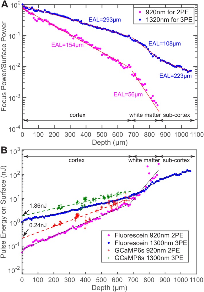
Figure 1.
Comparison of the power attenuation of 1320 nm and 920 nm excitation light and their respective 3-photon and 2-photon excitation efficiency in the mouse brain.
( A ) Power attenuation of 920 nm and 1320 nm excitation light in the mouse brain. The mouse brain vasculature was uniformly labeled with fluorescein dextran and imaged simultaneously by 920 nm 2PM an...
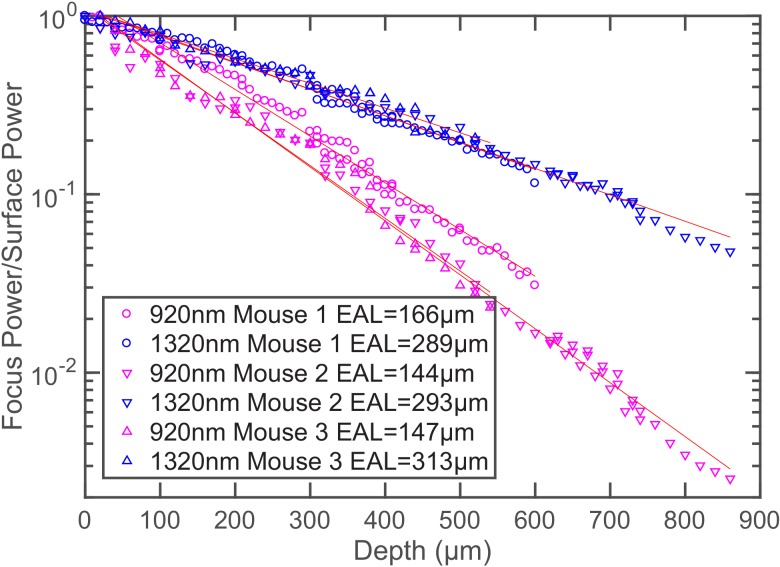
Figure 1u2014figure supplement 1.
Additional power attenuation curves of 920 nm and 1320 nm excitation light in the mouse neocortex (nu00a0=u00a03,u00a0>12 weeks old mice, all males).
Figure 1u2014figure supplement 1u2014source data 1. Additional power attenuation with depth curves of 1320 nm and 920 nm excitation light in the mouse neocortex, plotted in Figure 1u2014figure supplem...
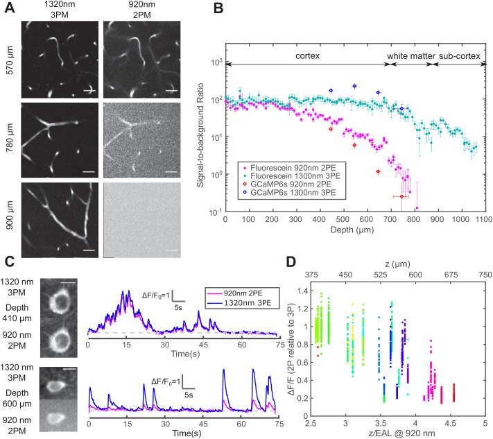
Figure 2.
Comparison of signal-to-background ratio for 1320 nm 3PM and 920 nm 2PM in the non-sparsely labeled mouse brain and its effect on calcium imaging sensitivity.
( A ) Comparison of 3PM and 2PM images of fluorescein-labeled blood vessels at different depths. Scale bar 30 u03bcm. ( B ) SBR measured simultaneously by 1320 nm 3PE and 920 nm 2PE on fluorescein-lab...
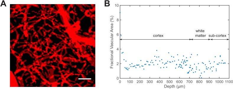
Figure 2u2014figure supplement 1.
Measurement of the staining density in uniformly labeled vasculature.
( A ) Z-projection of the identified blood vessels by summing all the XY-images in a vertical image stack (0u2013400 u03bcm deep, with 10 u03bcm step size). Scale bar, 30 u03bcm. ( B ) The fractional ...
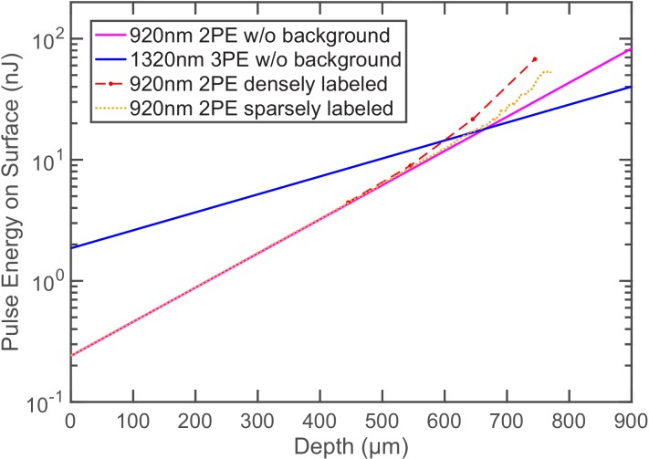
Figure 2u2014figure supplement 2.
The pulse energy required at the brain surface to generate the same d u2032 per pulse sampling the neuron for 2PE and 3PE of GCaMP6s at different imaging depths.
In the absence of the background fluorescence, d u2032 is entirely determined by signal photon counts: when a neuron is sampled by 1000 excitation pulses in 1 s, it generates F 0 = 1000 p u l s e s u0...
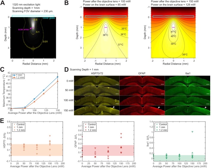
Figure 3.
Brain heating and thermal damage induced by continuous scanning by 1320 nm 3PM.
( A ) Monte Carlo simulation of light intensity of 1320 nm excitation light. The excitation light is focused at 1 mm below the brain surface in the cortex by an objective of 1.05 NA atu00a0~75% fillin...
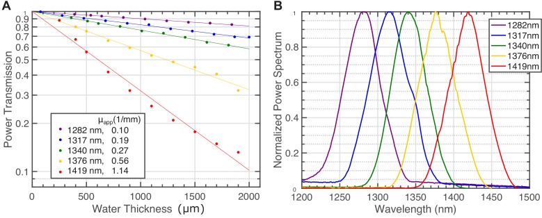
Figure 3u2014figure supplement 1.
Light attenuation by immersion water for various excitation wavelengths.
( A ) Power transmission versus immersion water thickness under the objective (Olympus XLPLN25XWMP2, 25X, NA=1.05, ~ 75% filling of the back aperture) for 5 spectra centered from 1280 nm to 1420 nm us...
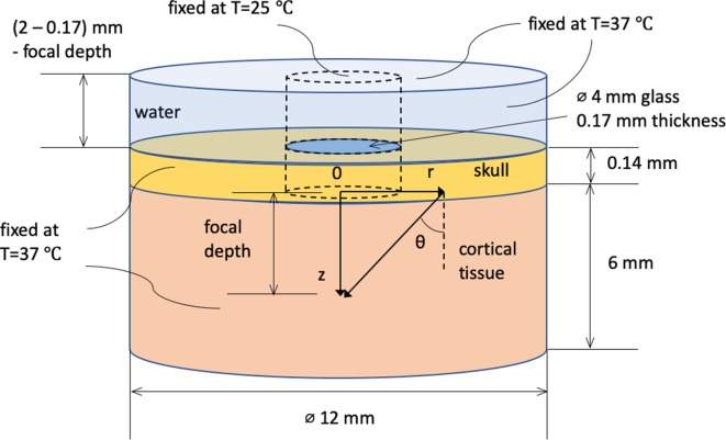
Figure 3u2014figure supplement 2.
Spatial dimension, coordinate system, and boundary conditions for Monte Carlo and heat conduction simulation.
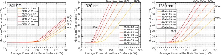
Figure 3u2014figure supplement 3.
The maximum brain temperature as a function of the average power at the brain surface, shown for different imaging depths at 920 nm, 1320 nm, and 1280 nm.
The imaging depth grows in the increment of the nominal EAL of the cortex, which is 150 u03bcm for 920 nm and 300 u03bcm for both 1320 nm and 1280 nm. The linear scanning FOV diameter is 300 u03bcm, a...
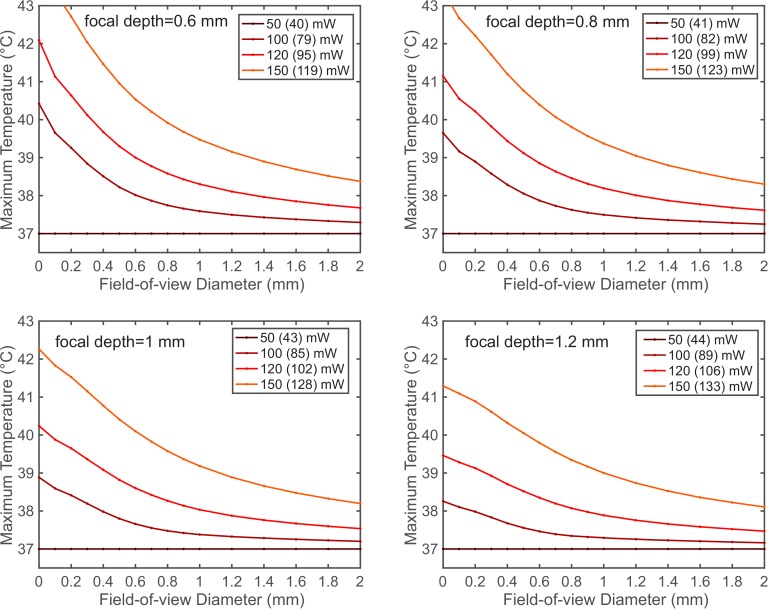
Figure 3u2014figure supplement 4.
The maximum brain temperature decreases with the scanning field-of-view.
The simulation was performed for 1320 nm excitation wavelength at 1- and 1.2 mm imaging depth with various average powers after the objective lens. The NA and the back-aperture beam size remain the sa...
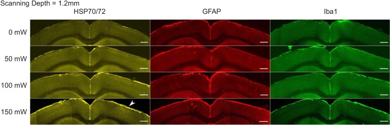
Figure 3u2014figure supplement 5.
Immunostaining reveals brain tissue damage by 1320 nm 3PM with 150 mW imaging power after the objective lens at 1.2 mm imaging depth.
The scanning was performed with 230 u03bcm FOV for 20 min at various average powers in the mouse brain. The window and scanning area are on the right side of each brain slice, and the location of heat...
Figure images are served from the NIH/NLM PubMed Central Open Access Subset or Europe PMC; copyright remains with the publishers and authors.
💬 Discussion
0 commentsNo comments yet. Be the first to start a discussion!
Leave a Comment