Abstract
Due to the overlapping emission spectra of fluorophores, fluorescence microscopy images often have bleed-through problems, leading to a false positive detection. This problem is almost unavoidable when the samples are labeled with three or more fluorophores, and the situation is complicated even further when imaged under a multiphoton microscope. Several methods have been developed and commonly used by biologists for fluorescence microscopy spectral unmixing, such as linear unmixing, non-negative matrix factorization, deconvolution, and principal component analysis. However, they either require pre-knowledge of emission spectra or restrict the number of fluorophores to be the same as detection channels, which highly limits the real-world applications of those spectral unmixing methods. In this paper, we developed a robust and flexible spectral unmixing method: Learning Unsupervised Means of Spectra (LUMoS), which uses an unsupervised machine learning clustering method to learn individual fluorophores' spectral signatures from mixed images, and blindly separate channels without restrictions on the number of fluorophores that can be imaged. This method highly expands the hardware capability of two-photon microscopy to simultaneously image more fluorophores than is possible with instrumentation alone. Experimental and simulated results demonstrated the robustness of LUMoS in multi-channel separations of two-photon microscopy images. We also extended the application of this method to background/autofluorescence removal and colocalization analysis. Lastly, we integrated this tool into ImageJ to offer an easy to use spectral unmixing tool for fluorescence imaging. LUMoS allows us to gain a higher spectral resolution and obtain a cleaner image without the need to upgrade the imaging hardware capabilities.
🔬 Techniques
💻 Software
✨ Fluorophores
🧪 Sample Preparation
🔬 Cell Lines
🏭 Microscope Brands
🧪 Reagent Suppliers
🔴 Lasers
📷 Detectors
💻 Software Details
💾 Data Repositories
🏷️ Research Resource Identifiers (RRIDs)
Verified research resources used in this paper:
🏛️ Research Organizations (ROR)
Affiliated research institutions:
📋 Methods
Sample preparations For N fluorophores = N detectors unmixing studies, FluoCells Prepared Slide #1 ( F36924 , Invitrogen, Carlsbad, CA) was used. Fixed bovine pulmonary artery endothelial (BPAE) cells were stained with a combination of fluorescent dyes. DAPI was used to label the nuclei, F-actin was stained using Alexa Fluor488 (AF488) phalloidin, and mitochondria were labeled with MitoTracker Red CMXRos. For N fluorophores > N detectors beads unmixing studies, particles of different sizes and colors were mixed and prepared on a glass slide and covered with a #1 cover slip for imaging. The commercial beads were either surface conjugated with standard fluorophores or polymerized with an organic dye within. The emission (EM) peak was either determined by the online spectra-viewer for a standard fluorophore or provided by the nanoparticle company (Spherotech Inc., Lake Forest, IL) for an organic dye. A combination of 5 different beads was used: Light Yellow (LY, FP-2045-2, Spherotech Inc.): 1.97μm in diameter, 450nm peak EM; FITC (ECFP-F1, Spherotech Inc.): 3.27μm in diameter, 515nm peak EM; PE (ECFP-F2, Spherotech, Inc.): 3.4μm in diameter, 575nm peak EM; Purple (FP-2062-2, Spherotech Inc.): 2.37μm in diameter, 620nm peak EM; APC (345036, BD Biosciences, San Jose, CA): 6μm in diameter, 660nm peak EM. For N fluorophores > N detectors Colorful Cell unmixing studies, a plasmid encoding 6 independent transcription units driving expression of different fluorescent proteins to distinct intracellular compartments, Colorful Cell [ 33 ], was a gift from Pierre Neveu (RRID:Addgene_62449; http://n2t.net/addgene:62449 ; Addgene, Watertown, MA). The 6 fluorescent proteins were TagBFP trimer fused to a nuclear localization sequence, Cerulean trimer fused to a plasma membrane targeting sequence, AzamiGreen fused to a mitochondrial localization sequence, Citrine fused to a Golgi targeting sequence, mCherry fused to an endoplasmic reticulum retention sequence, and iRFP670 fused to a peroxisome localization sequence. Plasmid DNA was transiently transfected into HEK293T (Pheonix) cells by calcium phosphate precipitation and assayed 48–72 hours later. By flow cytometry 40–70% of cells were expressing the transfected plasmid. For imaging, wet mounts of single cell suspensions containing 100,000 live cells/10 μL were prepared and imaged immediately. For the colocalization experiments, CD28-deficient, DO11.10 T cells were retrovirally transduced with CD28 fused at the C terminus to YFP or to Cerulean either separately or together. T cells were then mixed with stably transfected antigen-presenting cells (APCs) expressing MHC class II, ICAM-1, and CD80 that were or were not preloaded with 2.0 μg/ml OVA peptide for 1 hour at 37°C, and pelleted at Rcf 2000 for 20 sec. The pellet was incubated at 37° C for 10 min, resuspended and plated on poly-L–lysine coated cover slips for imaging [ 34 ].
Show full methods section
Sample preparations For N fluorophores = N detectors unmixing studies, FluoCells Prepared Slide #1 ( F36924 , Invitrogen, Carlsbad, CA) was used. Fixed bovine pulmonary artery endothelial (BPAE) cells were stained with a combination of fluorescent dyes. DAPI was used to label the nuclei, F-actin was stained using Alexa Fluor488 (AF488) phalloidin, and mitochondria were labeled with MitoTracker Red CMXRos. For N fluorophores > N detectors beads unmixing studies, particles of different sizes and colors were mixed and prepared on a glass slide and covered with a #1 cover slip for imaging. The commercial beads were either surface conjugated with standard fluorophores or polymerized with an organic dye within. The emission (EM) peak was either determined by the online spectra-viewer for a standard fluorophore or provided by the nanoparticle company (Spherotech Inc., Lake Forest, IL) for an organic dye. A combination of 5 different beads was used: Light Yellow (LY, FP-2045-2, Spherotech Inc.): 1.97μm in diameter, 450nm peak EM; FITC (ECFP-F1, Spherotech Inc.): 3.27μm in diameter, 515nm peak EM; PE (ECFP-F2, Spherotech, Inc.): 3.4μm in diameter, 575nm peak EM; Purple (FP-2062-2, Spherotech Inc.): 2.37μm in diameter, 620nm peak EM; APC (345036, BD Biosciences, San Jose, CA): 6μm in diameter, 660nm peak EM. For N fluorophores > N detectors Colorful Cell unmixing studies, a plasmid encoding 6 independent transcription units driving expression of different fluorescent proteins to distinct intracellular compartments, Colorful Cell [ 33 ], was a gift from Pierre Neveu (RRID:Addgene_62449; http://n2t.net/addgene:62449 ; Addgene, Watertown, MA). The 6 fluorescent proteins were TagBFP trimer fused to a nuclear localization sequence, Cerulean trimer fused to a plasma membrane targeting sequence, AzamiGreen fused to a mitochondrial localization sequence, Citrine fused to a Golgi targeting sequence, mCherry fused to an endoplasmic reticulum retention sequence, and iRFP670 fused to a peroxisome localization sequence. Plasmid DNA was transiently transfected into HEK293T (Pheonix) cells by calcium phosphate precipitation and assayed 48–72 hours later. By flow cytometry 40–70% of cells were expressing the transfected plasmid. For imaging, wet mounts of single cell suspensions containing 100,000 live cells/10 μL were prepared and imaged immediately. For the colocalization experiments, CD28-deficient, DO11.10 T cells were retrovirally transduced with CD28 fused at the C terminus to YFP or to Cerulean either separately or together. T cells were then mixed with stably transfected antigen-presenting cells (APCs) expressing MHC class II, ICAM-1, and CD80 that were or were not preloaded with 2.0 μg/ml OVA peptide for 1 hour at 37°C, and pelleted at Rcf 2000 for 20 sec. The pellet was incubated at 37° C for 10 min, resuspended and plated on poly-L–lysine coated cover slips for imaging [ 34 ].
Two-photon imaging
All images were collected by an Olympus FVMPE-RS system (Olympus, Center Valley, PA) using Olympus 25× water objective (XLPLN25XWMP2, 1.05NA). The system was equipped with two two-photon lasers: Spectra-Physics InSightX3 (680nm-1300nm, Spectra-Physics, Santa Clara, CA) and Spectra-Physics MaiTai DeepSee Ti:Sapphire laser (690nm-1040nm). There were four Photon Multiplier Tubes (PMTs) and two filter cubes for multi-color imaging. Galvanometer scanners were used for scanning. PMT gains for all imaging were used between 500 and 650 a.u. in the Olympus Fluoview software. The system schematic is shown in S1 Fig (the Blue/Green, and Red/fRed filter cubes setup is shown). For N fluorophores = N channels unmixing studies, FluoCells Prepared Slide #1 was imaged using MaiTai laser at 780nm to excite DAPI, AF488, and MitoTracker Red in the BPAE cells. 3D 512x512 pixel images were collected with 0.5μm per z step. For N fluorophores >N channels beads unmixing studies, multi-color beads slide was imaged using InSightX3 laser at 1000nm and MaiTai laser at 800nm simultaneously. 2D 512×512 pixel images were collected. For N fluorophores >N channels Colorful Cell separation studies, Colorful Cell slide was imaged using InSightX3 laser at 1050nm and MaiTai laser at 840nm sequentially with 1024×1024 pixels in x-y and 0.5μm per z step. Blue/Green cube (420-460nm/495-540nm) and red/fRed cube (575-630nm/645-685nm) were used for the above imaging. For colocalization studies, Cerulean, YFP, or Cerulean + YFP labeled cell slides were imaged with 800×800 pixels in x-y and 0.5μm per z step using InSightX3 laser at 970nm and MaiTai laser at 860nm sequentially. CFP/YFP cube (420-500nm/519-549nm) was used for this colocalization experiment. Data pre-processing Depending on the content of the input image, it may be appropriate to group together pixels with different net intensities but similar ratios of intensities in different z-planes. This could be necessary in fluorescence microscopy, and especially 2PLSM, in which there usually are signal intensity differences across imaging depths. This can be accounted for by dividing the intensity of a pixel x in each channel c by the overall sum of that pixel intensities across all the channels: x ^ c = x c ∑ c ∈ C x c (1) where x c is the raw intensity of pixel x in channel c , x ^ c is the scaled intensity of pixel x in channel c and C is the set of all input channels. This step is not always desirable, as in some cases pixels with the same intensity ratios but different raw intensities may actually represent different structures. To prevent the clustering algorithm from being biased by signal intensity differences and variations between channels, the brightness and contrast of input data were normalized to be relatively spherical distributions before clustering. Normalization also makes k -means initialize with better centroid choices and run faster with fewer iterations to converge [ 32 , 35 ]. Therefore, clustering was performed on z -scores where the z -score is the number of standard deviations away from the mean a signal. This can be expressed for a given pixel x as: z x , c = x ^ c − μ c σ c (2) where z x , c is the z -score for pixel x in channel c , and μ c and σ c are the overall mean and standard deviation of all pixels in channel c . This can be done to pixels with either non-scaled intensities ( x c ) or scaled intensities ( x ^ c ) as in Eq1.
LUMoS algorithm
We here present an unsupervised machine learning clustering method (Learning Unsupervised Means of Spectra, LUMoS) to learn the spectral signatures of each fluorophore and assign each pixel to the cluster whose spectral signature is closest. The process is referred to as “unsupervised” because no human intervention is required to label any pixels as belonging to a particular fluorophore, and the algorithm can identify features from raw images simply by looking at the pixels’ intensity values across all the detection channels. Specifically, a hard clustering method, k -means clustering, was used to separate mixed fluorophores unambiguously. Pixels that are spatially close tend to belong to the same structure, and thus stained by the same fluorophore. To leverage this spatial information to improve the unmixing ability of LUMoS beyond the single-pixel level, a median filter (3×3×3 or 5×5×5) is first applied to the image before clustering. In order to preserve potentially meaningful variations in intensity in the raw image, the median filter is only applied at the clustering stage and the intensity output for each pixel is still taken from the raw image. Given a set of observations X , containing n individual observations: x 1 , x 2 , …, x n , the objective of k -means is to partition all observations into k different clusters, S = { S 1 , S 2 ,…, S k }, in a way that minimizes within-cluster variance. This can be expressed as min s ∑ x ∈ X m i n i ‖ x − s i ‖ 2 (3) where s i is the centroid of cluster S i . Unlike other applications where k is difficult to define and requires tuning to optimize, in our case, the number of clusters k is simply the total number of fluorophores plus 1 more cluster that represents the background. The cluster centroid resulting from this approach can be interpreted as the spectral signatures of each fluorophores. These are the spectral means alluded to in the name Learning Unsupervised Means of Spectra (LUMoS) . The algorithm partitions the data into k clusters using Eq3 as a loss function. K -means approximates the solution to minimize the loss function by assigning data points to the class to whose centroid they are closest, and iteratively updating the centroid. Fig 1 details the steps taken in LUMoS. There are several algorithms for initializing the cluster centroids and we implemented the k -means++ initialization algorithm for its speed and convergence properties [ 36 ]. Briefly, k -means++ chooses the first cluster centroid at random from the input data points, and each subsequent cluster centroid is selected from the remaining data points with the probability inversely related to the distance from the closest appointed centroid. The algorithm converges when clusters do not change following one iteration. The maximum number of iterations allowed per replicate, max_iter , was set to 100 to limit run time. The iterative algorithm was applied num_replicates times and the replicate with the lowest cost was used in accordance with the loss function given in Eq3. All the unmixing performed in this paper used 10 replicates. The values of num_replicates and max_iter can be tuned, with more replicates and iterations yielding higher quality results but longer runtime. 10.1371/journal.pone.0225410.g001 Fig 1 LUMoS spectral unmixing algorithm. Once the algorithm converges, a new output image is created with k channels where each channel belongs to one cluster. In the output image, a pixel x assigned to one channel c is given the value of the highest intensity of that pixel among all the C input channels, and any pixel not belonging to channel c is assigned a value of 0: y i = { max c ∈ C x c i f p i x e l y b e l o n g s t o c l u s t e r S i 0 otherwise (4) where y i is the intensity of output pixel y in output channel i . At its core, spectral unmixing is the task of decomposing mixed multichannel images into spectral signatures and abundances of each signature in each pixel [ 9 , 37 , 38 ]: [ X 1 , 1 ⋯ X 1 , n ⋮ ⋱ ⋮ X C , 1 ⋯ X C , n ] = [ A 1 , 1 ⋯ A 1 , k ⋮ ⋱ ⋮ A C , 1 ⋯ A C , k ] [ B 1 , 1 ⋯ B 1 , n ⋮ ⋱ ⋮ B k , 1 ⋯ B k , n ] (5) which may be simplified as: X = AB . In Eq5, X is the observed fluorescence intensities of n pixels in C different spectral channels. The endmembers are the known fluorophores used to label the sample. A is a C × k matrix of the spectral signatures for each of the k fluorophores, in which each column is the recorded intensity of a fluorophore across the C detection channels. B is a k × n matrix containing the abundances of each fluorophore in each pixel. In LUMoS unmixing, B is obtained by scaling each pixel’s class label to the original intensity of that pixel as described in Eq4, which is based on a binary assumption that each pixel is occupied by only one fluorophore. Unlike other linear unmixing algorithms, LUMoS unmixes based on clustering rather than directly solving Eq5 with linear methods; because of this, LUMoS is different in that 1) the prior knowledge of fluorophore spectra ( A ) is not required to do the inversion of the equation and calculate the abundances ( B ), 2) it is not required that the number of fluorophores or endmembers ( k ) must be less than the number of detection channels ( C ), and 3) the abundances ( B ) are not the fractions of all endmembers, but are binary results assuming one endmember per pixel (Eq4).
Synthetic data
In order to test the capabilities of LUMoS across a wide range of conditions, we generated synthetic data for unmixing. We assumed the hardware for the simulated imaging to be the same as our two-photon system with 2 two-photon lasers and 4 detection channels (blue: 420-460nm, green: 495-540nm, red: 575-630nm and far-red 645-685nm). For each simulated fluorophore, a theoretical emission spectrum was generated ( Fig 2A ). The intensity distribution was modeled as a Weibull distribution (Eq6) with a = 1.7 and b = 100 to reflect the tendency of a fluorochrome to have a long tail at the longer wavelength [ 37 ]. R e l a t i v e I n t e n s i t y = a b ( λ − c b ) a − 1 e − ( ( λ − c ) / b ) a (6) where λ is emission wavelength and c is a constant to shift the peak of the emission spectra for different synthetic fluorophores. 10.1371/journal.pone.0225410.g002 Fig 2 Synthetic data. (A) Synthetic emission spectra of 8 fluorophores. Bandwidth of the 4 detection channels were marked in shaded areas. For simplicity, the emission spectra of synthetic fluorophores were assumed to be the same Weibull distribution with the peaks of all fluorophores evenly distributed between 420nm and 685nm. (B) Spectral signatures of the 8 synthetic fluorophores in A. The intensity of each fluorophore was measured as the integrated area under the spectral curves in A. (C) Synthetic 2PLSM images based on the emission spectra in A. The ground truth image shows the 8 synthetic fluorophore expressing structures. Ch1-Ch4 images were the raw images from the 4 detection channels with an SNR of 10. Each fluorophore was synthetized to be expressed in a narrow band either vertically or horizontally. 7 of the 8 bands had the same area, while 1 small band (furthest red fluorophore) has an area 1/5 th (cluster size ratio 0.2) of the rest. The emission peaks were evenly spaced between 420nm and 685nm so that all fluorophore peaks fell within the detection range of the microscope. We assumed all fluorophores were excited effectively, and their emission spectra peak at the same magnitude. Consistent spectral shapes and spacing represented an ideal case for easy simulations, but in reality, fluorophores usually have different shapes of spectra or even multiple peaks. To facilitate the generation of a synthetic image for an arbitrary number of fluorophores, a grid pattern was created where each successive fluorophore occupies an alternating vertical or horizontal strip ( Fig 2C ). For this synthetic data, the ideal situation where each pixel is occupied by only one fluorophore is assumed, to mimic the general biological staining assumptions without considering the nano-scale colocalizations caused by spatial resolution limitations. This pattern is overlaid onto a background with no fluorophores present. All synthetic images were 512×512 pixels. The length and width of the strip of the furthest red fluorophore was set variable while the rest of fluorophore expressing strips were fixed to be 512 pixels long and 256 p i x e l s # o f f l u o r o p h o r e s wide. This allowed us to measure the performance of LUMoS with unbalanced structure sizes. Cluster size ratio was the area of the minor fluorophore strip (furthest red) divided by the area of the major fluorophore strip. Within each strip, all pixels belong to the same fluorophore but they all have slightly different emission spectra from the ideal value expressed in Eq6. Each pixel’s adjusted spectrum was shifted by a randomly selected wavelength with a standard deviation of 10nm to represent the variance present in real imaging. A four-channel representation of the pixel was then generated by integrating the emission spectrum within the bandpass of the detection channels ( Fig 2B ). For pixels with no fluorophore, a small background noise was added from a Gaussian distribution with a mean of 2 and standard deviation of 1. Additional Poisson noise was then applied to each channel to mimic the shot noise. At the end, the image was convolved with a Gaussian filter with a standard deviation of 0.5 and a 3×3 median filter to represent real-world diffusion effects. Synthetic data unmixing performance was evaluated with the F1 score between the LUMoS output and the ground truth image ( Fig 2C ): F 1 = 2 × p r e c i s i o n * r e c a l l p r e c i s i o n + r e c a l l (7) where p r e c i s i o n = t r u e p o s i t i v e s t r u e p o s i t i v e s + f a l s e p o s i t i v e s , and r e c a l l = t r u e p o s i t i v e s t r u e p o s i t i v e s + f a l s e n e g a t i v e s .
Supporting information S1 Fig Two-photon system schematic. The system (Olympus FVMPE-RS) was equipped with two two-photon lasers and four PMTs. 25× water immersion objective was used. M: mirror, DM: dichroic mirror, Scanner: galvanometer scanner, PMT: photomultiplier tube. The Blue/Green (420-460nm/495-540nm), and Red/fRed (575-630nm/645-685nm) filter cubes setup is shown. (TIF) Click here for additional data file. S2 Fig Single stained cell preparations of the colocalization example. T cells only transduced with Cerulean or YFP virus mixed with APCs and imaged with the same conditions as in Fig 6 . (A) Cells transduced with Cerulean expressing virus. Cerulean signals showed only in CFP channel (Ch1). (B) Cells transduced with YFP virus. YFP signals were only detected by the YFP channel (Ch2). There was no cross-talk between CFP and YFP channels. APCs showed weak autofluorescence. (TIF) Click here for additional data file. S3 Fig Separated background noise cluster images. (A) The separated background image by LUMoS of the BPAE cells image in Fig 3 . (B) The separated background image by LUMoS of the multi-color beads image in Fig 4 . (C) The separated background image by LUMoS of the colorful cell image in Fig 5 . (D) The separated background image of the imaged cells in Fig 6 . (TIF) Click here for additional data file. S4 Fig Two-fluorophore peak distance limitations. (A) Synthetic emission spectra of two fluorophores with peak emissions at 475 nm and 490 nm. 10 nm standard deviations for each spectra are shown in shaded area. (B) The performance of LUMoS for synthetic images of two fluorophores with variable distances between emission peaks. The cluster size ratio was fixed at 0.2, number of fluorophores at 2 and SNR at 10. For each color plotted, the peak of the lower wavelength fluorophore was fixed while the peak of the higher wavelength fluorophore was varied. Results of 10 simulations were averaged to obtain the final results. (TIF) Click here for additional data file. S1 Movie BPAE cells 3D image unmixing results. Z-stack of BPAE cells 2PLSM images shown in Fig 3 . Left , raw image. Right , LUMoS unmixed image. (MOV) Click here for additional data file. S2 Movie Colorful Cell 3D image unmixing results. Z-stack of Colorful Cell cells 2PLSM images shown in Fig 5 . Left , raw image. Right , LUMoS unmixed image. (MOV) Click here for additional data file. S3 Movie Cerulean and YFP colocalization 3D image unmixing results. Z-stack of T cells transduced with Cerulean and YFP virus shown in Fig 6 . Top , raw image. Bottom , LUMoS unmixed image. (MOV) Click here for additional data file.
📊 Figures
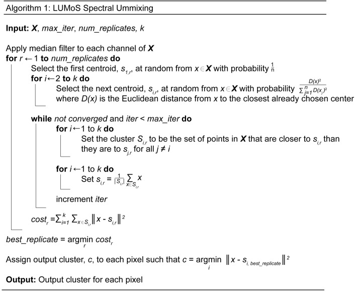
Fig 1
LUMoS spectral unmixing algorithm.
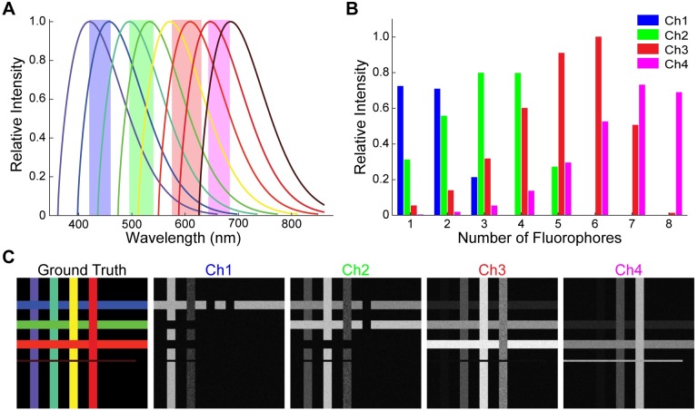
Fig 2
Synthetic data.
(A) Synthetic emission spectra of 8 fluorophores. Bandwidth of the 4 detection channels were marked in shaded areas. For simplicity, the emission spectra of synthetic fluorophores were assumed to be t...
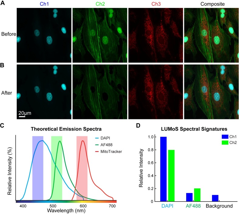
Fig 3
LUMoS unmixing of BPAE cells with channels bleed-through.
(A) BPAE cell stained with DAPI in nuclei, AF488 in actin, and MitoTracker Red in mitochondria, and imaged with 2PLSM. Images shown were 2D maximum intensity projections of 3D z-stacks. The green chan...
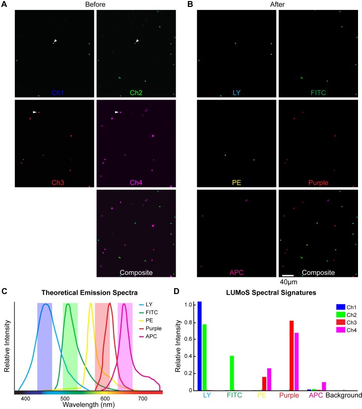
Fig 4
LUMoS unmixing of 5-color beads mixed in 4 detection channels.
(A) Mixed beads stained with Light Yellow (LY), FITC, PE, Purple, and APC imaged with 2PLSM. LY and Purple are special dyes by Spherotech. It was unable to resolve 5 colors with 4 detectors, and there...
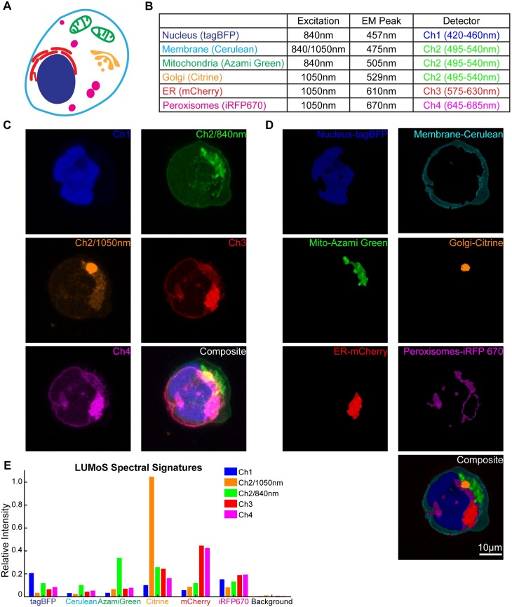
Fig 5
LUMoS unmixing of the colorful cell expressing 6 colors.
(A) Schematic of the Colorful Cell expressing BFP in nucleus, Cerulean in cell membrane, AzamiGreen in mitochondria, Citrine in Golgi bodies, mCherry in endoplasmic reticulum, and iRFP 670 in peroxiso...
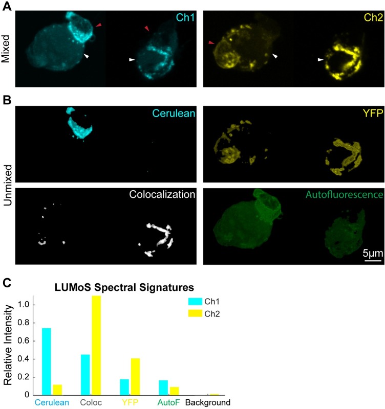
Fig 6
LUMoS unmixing for colocalization analysis and autofluorescence removal.
(A) The raw 2-channel 2PLSM images of T cells expressing Cerulean, YFP, or colocalized Cerulean and YFP. APCs are larger cells (pointed out by white arrows) than T cells (pointed out by red arrows), a...
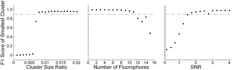
Fig 7
Simulation tests of the performance of LUMoS.
Left , the performance of LUMoS with unbalanced structure size. The number of fluorophores was fixed at 8 and SNR at 10. Middle , the performance of LUMoS with increasing number of fluorophores. The c...
Figure images are served from the NIH/NLM PubMed Central Open Access Subset or Europe PMC; copyright remains with the publishers and authors.
💬 Discussion
0 commentsNo comments yet. Be the first to start a discussion!
Leave a Comment