Abstract
Stress granules (SGs) are cytosolic, nonmembranous RNA-protein complexes. In vitro experiments suggested that they are formed by liquid-liquid phase separation; however, their properties in mammalian cells remain unclear. We analyzed the distribution and dynamics of two paradigmatic RNA-binding proteins (RBPs), Ras GTPase-activating protein SH3-domain-binding protein (G3BP1) and insulin-like growth factor II mRNA-binding protein 1 (IMP1), with single-molecule resolution in living neuronal cells. Both RBPs exhibited different exchange kinetics between SGs. Within SGs, single-molecule localization microscopy revealed distributed hotspots of immobilized G3BP1 and IMP1 that reflect the presence of relatively immobile nanometer-sized nanocores. We demonstrate alternating binding in nanocores and anomalous diffusion in the liquid phase with similar characteristics for both RBPs. Reduction of low-complexity regions in G3BP1 resulted in less detectable mobile molecules in the liquid phase without change in binding in nanocores. The data provide direct support for liquid droplet behavior of SGs in living cells and reveal transient binding of RBPs in nanocores. Our study uncovers a surprising disconnect between SG partitioning and internal diffusion and interactions of RBPs.
🔬 Techniques
💻 Software
✨ Fluorophores
🧪 Sample Preparation
🔬 Cell Lines
🏭 Microscope Brands
🧪 Reagent Suppliers
📷 Detectors
💻 Software Details
💻 Code & Software
💾 Data Repositories
🏛️ Research Organizations (ROR)
Affiliated research institutions:
📋 Methods
Constructs and materials Eukaryotic expression plasmids for human G3BP1 and human IMP1 with amino-terminally fused HaloTag and SNAP-tag were constructed from pRc/cytomegalovirus (CMV)–based expression vectors coding for PAGFP- and mCherry-tagged G3BP1 and IMP1 ( Moschner et al., 2014 ). The coding sequence for human G3BP1 was PCR amplified from pRc/CMV PAGFP-hG3BP1 and modified to include a SbfI and a NotI restriction site using the primers Sbf1_G3BP1_FW and G3BP1_NotI_BW (5′-GGCCCCTGCAGGGATGGTGATGGAGAAG-3′/5′-GTTATCTAGATGCGGCCGCTCACTGCCGTG-3′). The PCR product as well as the vector plasmid pSems HaloTag-hTau441wt were digested using SbfI and NotI endonucleases, followed by ligation. Cloning of SNAP-tag-hG3BP1 was performed essentially the same using pSems fSNAP-tag-Rab5a as vector. The coding sequence for IMP1 was PCR amplified from pRc/CMV PAGFP-IMP1 and modified to include a XhoI and a NotI restriction site using the primers XhoI_IMP1_FW and IMP1_NotI_BW (5′-CGCGGGCTCGAGATATCCATGAACAAG-3′/5′-CCGGCGGCCGCTCACTTCCTCCG-3′). The PCR product and the vector plasmid pSems haloTag-hTau441wt were digested using XhoI and NotI endonucleases, followed by ligation. To clone pSems SNAP-tag-IMP1, the vector pSems fSNAP-tag-Rab5a and the plasmid pSems HaloTag-IMP1 were linearized using XhoI and NotI endonucleases, followed by ligation. The pCMV-3×PAGFP plasmid ( Weissmann et al., 2009 ) and the construct coding for mEGFP-HaloTag ( Wedeking et al., 2015 ) were described previously. The deletion constructs G3BP1 N , G3BP1 C and IMP1 C were prepared as described previously ( Moschner et al., 2014 ). Sequences that were introduced by PCR were verified by DNA sequencing (Seqlab-Microsynth). Chemicals were obtained from Sigma-Aldrich, and cell culture media, supplements, culture flasks, plates, and dishes were obtained from Sigma-Aldrich and ThermoFisher Scientific, unless stated otherwise. TMR-HTL was obtained from Promega, JF549-HTL and PA-JF549-HTL from Janelia Research Campus (Ashburn, VA), and SiR (SNAP-Cell 647-SiR) from New England Biolabs. The following antibodies were used: anti–TIA-1 (G-3; mouse monoclonal; Santa Cruz Biotechnology), anti-G3BP1 (NBP2; rabbit polyclonal; Novus Biologicals), anti-IMP1 (D-9; mouse monoclonal; Santa Cruz Biotechnology). As secondary antibodies, anti–mouse Alexa488 (Jackson ImmunoResearch Laboratories) or anti–rabbit and anti–mouse detection modules for Wes (ProteinSimple Wes; ProteinSimple) were used.
Show full methods section
Constructs and materials Eukaryotic expression plasmids for human G3BP1 and human IMP1 with amino-terminally fused HaloTag and SNAP-tag were constructed from pRc/cytomegalovirus (CMV)–based expression vectors coding for PAGFP- and mCherry-tagged G3BP1 and IMP1 ( Moschner et al., 2014 ). The coding sequence for human G3BP1 was PCR amplified from pRc/CMV PAGFP-hG3BP1 and modified to include a SbfI and a NotI restriction site using the primers Sbf1_G3BP1_FW and G3BP1_NotI_BW (5′-GGCCCCTGCAGGGATGGTGATGGAGAAG-3′/5′-GTTATCTAGATGCGGCCGCTCACTGCCGTG-3′). The PCR product as well as the vector plasmid pSems HaloTag-hTau441wt were digested using SbfI and NotI endonucleases, followed by ligation. Cloning of SNAP-tag-hG3BP1 was performed essentially the same using pSems fSNAP-tag-Rab5a as vector. The coding sequence for IMP1 was PCR amplified from pRc/CMV PAGFP-IMP1 and modified to include a XhoI and a NotI restriction site using the primers XhoI_IMP1_FW and IMP1_NotI_BW (5′-CGCGGGCTCGAGATATCCATGAACAAG-3′/5′-CCGGCGGCCGCTCACTTCCTCCG-3′). The PCR product and the vector plasmid pSems haloTag-hTau441wt were digested using XhoI and NotI endonucleases, followed by ligation. To clone pSems SNAP-tag-IMP1, the vector pSems fSNAP-tag-Rab5a and the plasmid pSems HaloTag-IMP1 were linearized using XhoI and NotI endonucleases, followed by ligation. The pCMV-3×PAGFP plasmid ( Weissmann et al., 2009 ) and the construct coding for mEGFP-HaloTag ( Wedeking et al., 2015 ) were described previously. The deletion constructs G3BP1 N , G3BP1 C and IMP1 C were prepared as described previously ( Moschner et al., 2014 ). Sequences that were introduced by PCR were verified by DNA sequencing (Seqlab-Microsynth). Chemicals were obtained from Sigma-Aldrich, and cell culture media, supplements, culture flasks, plates, and dishes were obtained from Sigma-Aldrich and ThermoFisher Scientific, unless stated otherwise. TMR-HTL was obtained from Promega, JF549-HTL and PA-JF549-HTL from Janelia Research Campus (Ashburn, VA), and SiR (SNAP-Cell 647-SiR) from New England Biolabs. The following antibodies were used: anti–TIA-1 (G-3; mouse monoclonal; Santa Cruz Biotechnology), anti-G3BP1 (NBP2; rabbit polyclonal; Novus Biologicals), anti-IMP1 (D-9; mouse monoclonal; Santa Cruz Biotechnology). As secondary antibodies, anti–mouse Alexa488 (Jackson ImmunoResearch Laboratories) or anti–rabbit and anti–mouse detection modules for Wes (ProteinSimple Wes; ProteinSimple) were used.
Cell culture and transfections
PC12 cells were cultured in 15% serum/DMEM as described previously ( Fath et al., 2002 ). For induction of neuronal differentiation, the medium was switched to 1% serum/DMEM with 100 ng/ml 7 S mouse NGF (Alomone Laboratories) for 4 d. Transfections of PC12 cells were performed with Lipofectamine 2000 (Invitrogen) as described previously ( Fath et al., 2002 ). For FDAP analysis, cells were plated on 35-mm polylysine- and collagen-coated glass-bottom culture dishes (MatTek). For TIRF imaging, cells were plated on glass coverslips (24 mm, No. 1; VWR) that were coated with poly- l -lysine and collagen or poly- l -lysine–graft (polyethylene glycol)–copolymer functionalized with RGD as described previously ( Wedeking et al., 2015 ). Before imaging, the medium was exchanged against DMEM without phenol red. For the induction of stress, 0.5 mM sodium arsenite was added to the medium. After 20 min, the medium was replaced with fresh DMEM without phenol red. Labeling of cells for imaging was performed by incubation with serum-DMEM containing 0.5–5 nM TMR-HTL, 0.25 nM JF549-HTL, and 25 nM SiR for 20 min at 37°C. For photoactivation experiments with HaloTag constructs, PA-JF549-HTL was used at 100 nM. Subsequently, cells were washed 3 × 5 min with serum-DMEM without phenol red and transferred to the microscope.
Photoactivation and live cell imaging
Live cell imaging for FDAP experiments was performed on a laser scanning microscope (Eclipse TE2000-U inverted; Nikon) equipped with argon (488 nm), helium/neon (543 nm), and violet diode (407 nm) lasers. The microscope was enclosed in an incubation chamber maintained at 37°C and 5% CO 2 (Solent Scientific). A 60× magnification objective with NA 1.40 (oil, Plan Apo VC; Nikon) was used. Photoactivation was performed with the violet diode in a region between the nucleus and the cell membrane with a size of 3 × 5 µm. Automated image acquisition after photoactivation was essentially performed as described previously ( Weissmann et al., 2009 ). Frames were obtained at a frequency of 1 frame per second, and 112 frames were collected per experiment. Standard series were collected at a resolution of 256 × 256 pixels.
FDAP data analysis and fitting
For determination of fluorescence decay, individual image frames from FDAP experiments were extracted from raw images using Fiji software ( Schindelin et al., 2012 ). From all frames, the zero-level (“preactivation intensity”, t = −1 s) was subtracted to exclude the preactivation fluorescence and normalized to 1 by the maximal value at t = 0 s. Data fitting was performed using the Levenberg–Marquardt algorithm implemented in the Origin Pro 8 software package. To test for different fluorescence populations in the FDAP curves, two different model FDAP functions were used: I 1 ( t ) = F ∞ A + ( F 0 − F ∞ ) A e − t / τ , (1) and I 2 ( t ) = F ∞ ( A f a s t + A s l o w ) + ( F 0 − F ∞ ) A f a s t e − t / τ f a s t + ( F 0 − F ∞ ) A s l o w e − t / τ s l o w . (2) In Eq. 2 , A slow and A fast denote the relative fractions ranging from 0 to 1 of a slow and fast fraction, τ slow and τ fast represent the corresponding characteristic decay times of those fractions, and F ∞ and F 0 are auxiliary offset parameters. Eq. 1 is a simplification of Eq. 2, wherein the fraction of one of the two populations is set to 0. We underline that both models do not include information on either the geometry of the activation region or the molecular kinetics underlying the decay. Because there was no a priori knowledge whether a FDAP curve reflects the dynamic of one or two populations, both models were applied to fit every curve. The resulting fit parameters were averaged to produce a mean and SEM for each construct. By using a χ 2 statistical test to compare the results of fitting, it became clear that the FDAP curves for 3×PAGFP and PAGFP-IMP1 were better described by Eq. 1 and the curves for PAGFP-G3BP1 by Eq. 2 . Single-molecule microscopy, localization, and tracking For recording single molecules, TIRF microscopy was performed using an IX81 microscope (Olympus) with a four-line motorized TIR condenser (cellTIRF) and 405-nm (200 mW), 488-nm (200 mW), 561-nm (200 mW), and 642-nm (140 mW) lasers (Olympus). High-speed single-molecule tracking was performed using a digital scientific complementary metal–oxide–semiconductor camera (sCMOS, ORCA-Flash4.0 V2 C11440 -22CU; Hamamatsu). A 150× magnification objective with NA 1.45 (oil, UAPON 150×/1.45; Olympus) was used for TIR illumination in the highly inclined and laminated optical sheet mode. The emitted fluorescence from the sample was filtered using a quad-band bandpass filter (FF01 446/523/600/677; Semrock) and a secondary single bandpass filter: BrightLine HC 525/50 (Semrock) for meGFP, BrightLine HC 600/37 (Semrock) for TMR/JF549, and BrightLine HC 697/58 (Semrock) for SiR. The microscope was enclosed in an incubation chamber maintained at 37°C and 10% CO 2 (cellVivo; Olympus). Time series were recorded using Olympus CellSens 1.14 software. Cell vitality was confirmed by a bright field snapshot and double transfection verified with a snapshot in the SiR channel. Time series were performed in the TMR/JF549 channel with an exposure time of 10 ms and 2,000–8,000 frames were recorded per cell. Image stacks were imported using FIJI software ( Schindelin et al., 2012 ) and regions of interest containing RNP granules were cropped and saved as separate TIFF stacks that were further analyzed (∼2,000–6,000 frames, where individual molecules could be localized). Localization of single molecules and single-molecule tracking as well as further data processing were performed in MATLAB (MathWorks) using well-established localization and tracking algorithms as previously described ( Jaqaman et al., 2008 ; Sergé et al., 2008 ) implemented in a custom-written graphical user interface, which we call SLIMfast (software for localization-based imaging in MATLAB). The estimated localization precision achieved 20–30 nm in our experiments. Trajectory linking proceeded in parallel with the localization step and used a local criterion (a search radius determined by a hypothetical diffusion process) to build trajectories in each time step. Past statistics (instantaneous diffusion coefficient, mean intensity of spots, and blinking statistics) were taken into account when assigning new localized spots to trajectories to resolve local ambiguities such as crossing trajectories or dye blinking. Lifetime determination and diffusion in granules The trajectory set produced by SLIMfast contained, on the one hand, trajectories that existed for hundreds of frames and explored compact areas within granules. On the other hand, there were trajectories being rather short-lived but exploring wider areas. To separate those fractions from one another and estimate their relative abundances, the MSD for each trajectory longer than 10 frames was calculated and instantaneous diffusion coefficients were obtained by linearly fitting those MSDs between time lag 2 and 10. The distribution of diffusion constants was analyzed using a two-component Gaussian function to estimate the different populations. The Gaussians for the two subpopulations cross at a point ( D threshold ) that we defined as a border between those subpopulations. For trajectories that satisfied the inequality D < D threshold (defined as bound fraction), lifetime histograms were plotted and the mean lifetimes ( τ life ) were determined by fitting single exponential functions to them. The resulting lifetimes were corrected by subtracting an estimated bleaching rate γ (0.040 ± 0.002 s −1 ) from the corresponding dissociation rate 1/ τ life . For trajectories with instantaneous diffusion coefficients that satisfied the inverse inequality D > D threshold (defined as mobile fraction), MSD plots for time lags 2 to 20–40 were constructed. The MSDs were fitted by two models: simple and anomalous diffusion. In most cases, the MSD were better described by anomalous diffusion, which allowed us to determine the anomaly exponent α and diffusion constant Γ ( µm 2 /t α ) from the fits.
Cluster analysis
Clustering of localized molecule positions was performed using the DBSCAN algorithm ( Ester et al., 1996 ). This algorithm, given a set of points in 2D space, splits closely located points into groups (clusters) and rejects all unclustered points in low-density regions as “noise.” DBSCAN uses two parameters to define the critical density of points in a certain region to belong to a cluster, ε and m . A chosen point is a core sample when there exists at least m points within a circle of radius ε around a randomly chosen point in the set. The core (a set of closely packed core samples) is then recursively expanded by ensuring the validity of the aforesaid criterion for all neighboring points unless the local density of points drops significantly. Every detected cluster is surrounded by noncore samples that do not yet belong to noise but contain at least one core sample within their ε-neighborhood. To prepare single-molecule data for the cluster analysis, we performed the localization of TMR and SiR stacks using SLIMfast without any subsequent tracking (see Single-molecule microscopy, localization, and tracking). The coordinates of the localized positions of every granule were saved in ASCII format and were further analyzed by self-written Python scripts ( Oliphant, 2007 ) implementing the scikit-learn library for machine learning ( Pedregosa et al., 2011 ). Before working with experimental data, the cluster detection procedure was tested on simulated data to find optimal DBSCAN parameters (Fig. S5 A), which depend on factors such as the mean distance between points, the mean distance between clusters and the amount of noise in low-density regions. A general idea about the spatial scales present in a set of points can be given by the radial distribution function (RDF) which describes how the density of points changes as a function of distance from an arbitrary reference particle. As the test set is rather inhomogeneous, the RDF is expected to have a local maximum at low values of ε, which corresponds to the mean half-radius of high-density regions (future clusters). It is clear that the value of ε during the DBSCAN cluster detection should lie below this critical value ε*. In the opposite case, DBSCAN will ignore fine intracluster details and underestimate the number of detected clusters. Integrating the RDF over ε and multiplying it by the total number of points in the set yields the mean number of points within a circle of radius ε, ( ε ) . This information is required to estimate the optimal m parameter for the DBSCAN cluster detection. Choosing m close to ( ε ) ensures that the density of points for the chosen optimal value of ε is directly related to the composition of the given set of points. Given an optimal area in the (ε , m )-space for the DBSCAN cluster detection (0 < ε < ε * and m = ( ε ) ), one finally has to choose an appropriate pair of the parameters to perform the final clustering with. For every pair (ε i , ( ε i ) ), the number of clusters N clusters detected by DBSCAN was calculated (Fig. S5 A). N clusters decayed with the increase of ε, but not monotonously. There was, as expected, a sharp drop in N clusters when ε crossed the critical value ε * . This drop corresponds to a sort of “phase transition” as the fine intracluster details are not properly taken into account anymore. The sharp drop observed at small values of ε reflected an overestimation of the number of clusters because of the too high density required to classify points of clusters, which resulted in splitting of the actual clusters into smaller subclusters. The sought optimal parameter pair was therefore located in the plateau between the two drops of N clusters . Cluster detection with these parameters yield the best result for the given set of points (Fig. S5 B). To calculate the overlap area between two cluster sets (e.g., 1 and 2), we performed the binarization of the 2D space (Fig. S5 C). For this to be done, a 2D grid with a certain cell size ( d ) was created and put on the 2D space containing the cluster sets. The grid corresponded to a matrix whose elements were assigned 1 depending on whether the respective cell in the 2D grid contained core elements of both cluster sets. In all other cases, the elements of the matrix were assigned 0. The overlap area was then calculated as the number of all nonzero elements of the grid matrix n times the area of a single binarization cell d 2 . To eliminate the dependence of the overlap area on the cell size and account for different numbers of points in the cluster sets, a unitless measure s was introduced: s = n d 2 / S 1 S 2 , where S 1 and S 2 are the areas taken by the cluster set 1 and 2, respectively. To validate the values of the weighted overlap, we performed two types of calculations. First, using the datasets for TMR-G3PB1 and SiR-G3BP1 ( Fig. 3 C , first line), we selected signals that did not belong to any cluster detected with DBSCAN. Those signals were hence interpreted as noise. Calculating the weighted overlap for these noise contributions from the TMR and SiR channels yielded a value of 0.020 ± 0.001 (mean ± SEM, n = 8). Hence, noise detected in the different channels was spatially uncorrelated. Second, we calculated the weighted overlap between images, where the signals were generated numerically using a 2D uniform distribution and the total number of signal in either channel was comparable to that observed experimentally. This yielded 0.001 ± 0.000 (mean ± SEM, n = 8). This suggested that the measured overlaps in Fig. 3 C were significantly different from noise.
Analysis of quasistationary multiple binding sites
Nanocore binding sites within the SGs are expected to be quasistationary within the observed time period. Therefore binding events to such sites correspond to transient immobilization of G3BP1 and IMP1 and were detected using the DBSCAN principle as described above but adapted to work only within a constraint time window around each localization. Before localization, raw image stacks were preprocessed using a highly localized 3 × 3 × 3 median filter (width [pixels] × height [pixels] × depth [frames]) to specifically increase the signal to noise ratio of the immobilized particles. We then scanned around each localization within a radius ε of 225 nm (five times the apparent localization precision as determined from manually preselected binding events) tolerating a 50% probability to not observe the respective molecule because of blinking. We started with a time window of 30s (3,000 frames) to pick up prolonged binding events and sequentially reduced the time window to 1s (100 frames) to be able to detect more transient events but still discriminate mobile particles. Precise detection of the starting point and endpoint of the immobilization events was realized by initially clustering the localizations in a pure forward- or backward-looking sweep (for a point localized at time t 0 only those points localized at t > t 0 are considered in the forward sweep and vice versa in the backward sweep) and subsequent fusion of corresponding cluster via maximal overlap. Spurious start and end points caused by noise peaks were removed by enforcing at least three subsequent localizations to be present at these points. If the endpoint of one cluster coincided with the starting point of a second cluster within a radius of 500 nm and 1 s, then these clusters were subsequently merged into one. To determine the number of binding sites present, we extracted for each cluster the x-t- and y-t-kymographs and applied the STaSI algorithm to each coordinate ( Shuang et al., 2014 ). This algorithm decomposed the observed kymographs into an optimal number of piece-wise constant periods. The averages of these piece-wise constant periods in both dimensions then represent the position of the respective binding sites and their change points the sequential hopping of the RBPs from one binding site to the next. Because the binding sites showed some form of additional fluctuation, we set the minimum accepted jump distance to 90 nm (two times the apparent localization precision). To approximate the size of the nanocore, we calculated the pairwise distances between binding sites within one nanocore among selected samples.
Other methods
PC12 cells transfected with PAGFP-G3BP1 or PAGFP-IMP1 constructs were lysed with RIPA buffer containing protease inhibitors as described previously ( Moschner et al., 2014 ). Lysates were analyzed in the Simple Western size-based capillary electrophoresis system (ProteinSimple Wes) following the manufacturer’s instructions. Electropherograms were represented as pseudo-blots, generated using the inbuilt Compass software (ProteinSimple).
Statistical analysis
Statistical analysis among experimental groups was performed using Student’s t test. One-way ANOVA followed by post-hoc Tukey’s test for multiple comparisons was used for FDAP analysis (*, P < 0.05; **, P < 0.01; ***, P < 0.001). Online supplemental material Fig. S1 shows single-molecule imaging of G3BP1 and IMP1 in different combinations and examples of spatial clustering of single molecule localizations. Fig. S2 shows single-molecule imaging of mEGFP-HaloTag in living cells and single molecule imaging of fixed samples after expression of SiR-labeled SNAP-IMP1 and TMR-labeled HaloTag-G3BP1. Fig. S3 shows RNP-binding dynamics on a single-nanocore level. Fig. S4 shows localizations, trajectories, and biphasic partitioning of IMP1 within a SG and comparison of residence times for PAGFP-G3BP1 and PAGFP-IMP1 with the respective HaloTag constructs. Fig. S5 shows determination of optimal DBSCAN parameters for cluster detection using simulated data and lifetime determination of different combinations of HaloTag- and SNAP-tagged G3BP1 and IMP1 using the DBSCAN algorithm adapted to group localizations. Video 1 shows a visualization of DBSCAN algorithm adapted to group localizations that exhibit high spatiotemporal correlation. Video 2 shows single-molecule tracking of G3BP1 molecules in a SG. Video 3 shows TALM visualizing immobile hot spots of G3BP1 binding events. Video 4 shows single-molecule track of a G3BP1 molecule in a SG. Source code 1 shows custom-made Python scripts for detection of optimal DBSCAN parameters and analysis of G3BP1 and IMP1 clusters and colocalization. Source code 2 (available at https://github.com/CPaoloR/smDBSCAN/releases/tag/1.0-JCB ) shows MATLAB scripts for image smoothing, molecule localization, cluster analysis, kymograph extraction, and subsequent STaSI analysis for scrutinizing quasi-stationary multiple binding sites in SGs.
Constructs and materials Eukaryotic expression plasmids for human G3BP1 and human IMP1 with amino-terminally fused HaloTag and SNAP-tag were constructed from pRc/cytomegalovirus (CMV)–based expression vectors coding for PAGFP- and mCherry-tagged G3BP1 and IMP1 ( Moschner et al., 2014 ). The coding sequence for human G3BP1 was PCR amplified from pRc/CMV PAGFP-hG3BP1 and modified to include a SbfI and a NotI restriction site using the primers Sbf1_G3BP1_FW and G3BP1_NotI_BW (5′-GGCCCCTGCAGGGATGGTGATGGAGAAG-3′/5′-GTTATCTAGATGCGGCCGCTCACTGCCGTG-3′). The PCR product as well as the vector plasmid pSems HaloTag-hTau441wt were digested using SbfI and NotI endonucleases, followed by ligation. Cloning of SNAP-tag-hG3BP1 was performed essentially the same using pSems fSNAP-tag-Rab5a as vector. The coding sequence for IMP1 was PCR amplified from pRc/CMV PAGFP-IMP1 and modified to include a XhoI and a NotI restriction site using the primers XhoI_IMP1_FW and IMP1_NotI_BW (5′-CGCGGGCTCGAGATATCCATGAACAAG-3′/5′-CCGGCGGCCGCTCACTTCCTCCG-3′). The PCR product and the vector plasmid pSems haloTag-hTau441wt were digested using XhoI and NotI endonucleases, followed by ligation. To clone pSems SNAP-tag-IMP1, the vector pSems fSNAP-tag-Rab5a and the plasmid pSems HaloTag-IMP1 were linearized using XhoI and NotI endonucleases, followed by ligation. The pCMV-3×PAGFP plasmid ( Weissmann et al., 2009 ) and the construct coding for mEGFP-HaloTag ( Wedeking et al., 2015 ) were described previously. The deletion constructs G3BP1 N , G3BP1 C and IMP1 C were prepared as described previously ( Moschner et al., 2014 ). Sequences that were introduced by PCR were verified by DNA sequencing (Seqlab-Microsynth). Chemicals were obtained from Sigma-Aldrich, and cell culture media, supplements, culture flasks, plates, and dishes were obtained from Sigma-Aldrich and ThermoFisher Scientific, unless stated otherwise. TMR-HTL was obtained from Promega, JF549-HTL and PA-JF549-HTL from Janelia Research Campus (Ashburn, VA), and SiR (SNAP-Cell 647-SiR) from New England Biolabs. The following antibodies were used: anti–TIA-1 (G-3; mouse monoclonal; Santa Cruz Biotechnology), anti-G3BP1 (NBP2; rabbit polyclonal; Novus Biologicals), anti-IMP1 (D-9; mouse monoclonal; Santa Cruz Biotechnology). As secondary antibodies, anti–mouse Alexa488 (Jackson ImmunoResearch Laboratories) or anti–rabbit and anti–mouse detection modules for Wes (ProteinSimple Wes; ProteinSimple) were used.
Other methods
PC12 cells transfected with PAGFP-G3BP1 or PAGFP-IMP1 constructs were lysed with RIPA buffer containing protease inhibitors as described previously ( Moschner et al., 2014 ). Lysates were analyzed in the Simple Western size-based capillary electrophoresis system (ProteinSimple Wes) following the manufacturer’s instructions. Electropherograms were represented as pseudo-blots, generated using the inbuilt Compass software (ProteinSimple).
Online supplemental material Fig. S1 shows single-molecule imaging of G3BP1 and IMP1 in different combinations and examples of spatial clustering of single molecule localizations. Fig. S2 shows single-molecule imaging of mEGFP-HaloTag in living cells and single molecule imaging of fixed samples after expression of SiR-labeled SNAP-IMP1 and TMR-labeled HaloTag-G3BP1. Fig. S3 shows RNP-binding dynamics on a single-nanocore level. Fig. S4 shows localizations, trajectories, and biphasic partitioning of IMP1 within a SG and comparison of residence times for PAGFP-G3BP1 and PAGFP-IMP1 with the respective HaloTag constructs. Fig. S5 shows determination of optimal DBSCAN parameters for cluster detection using simulated data and lifetime determination of different combinations of HaloTag- and SNAP-tagged G3BP1 and IMP1 using the DBSCAN algorithm adapted to group localizations. Video 1 shows a visualization of DBSCAN algorithm adapted to group localizations that exhibit high spatiotemporal correlation. Video 2 shows single-molecule tracking of G3BP1 molecules in a SG. Video 3 shows TALM visualizing immobile hot spots of G3BP1 binding events. Video 4 shows single-molecule track of a G3BP1 molecule in a SG. Source code 1 shows custom-made Python scripts for detection of optimal DBSCAN parameters and analysis of G3BP1 and IMP1 clusters and colocalization. Source code 2 (available at https://github.com/CPaoloR/smDBSCAN/releases/tag/1.0-JCB ) shows MATLAB scripts for image smoothing, molecule localization, cluster analysis, kymograph extraction, and subsequent STaSI analysis for scrutinizing quasi-stationary multiple binding sites in SGs.
Supplementary Material Supplemental Materials (PDF) Python Source Code (ZIP file) Video 1 Video 2 Video 3 Video 4
📊 Figures
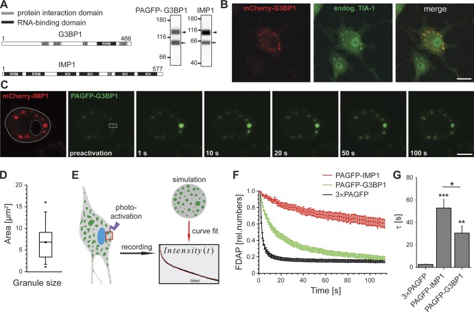
Figure 1.
G3BP1 and IMP1 exhibit different dynamics of protein exchange between SGs. (A) Protein interaction (gray) and RNA-binding domains (black) of human G3BP1 and IMP1 according to SMART analysis for identi...
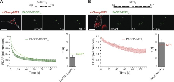
Figure 2.
Effect of G3BP1 and IMP1 deletions on protein exchange between SGs. (A and B) FDAP curves for PAGFP-G3BP1 C (A) and PAGFP-IMP1 C (B; mean u00b1 SEM, n = 22 and n = 13, respectively). Schematic represe...
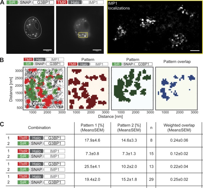
Figure 3.
G3BP1 and IMP1 are enriched in distributed nanocores within SGs. (A) Single-molecule imaging of SiR-labeled SNAP-G3BP1 and TMR-labeled HaloTag-IMP1. Snapshots before image acquisition confirmed the pr...
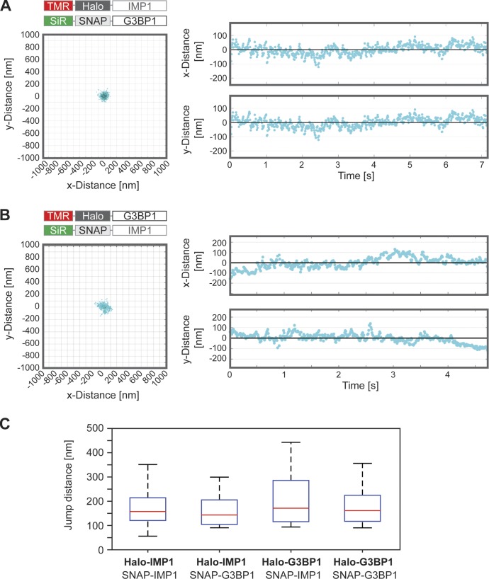
Figure 4.
Nanocores are relatively immobile within SGs and contain multiple binding sites. (A and B) Top view (left) and kymographic representation (right) of a typical single binding event of Halo-IMP1 on SNAP...
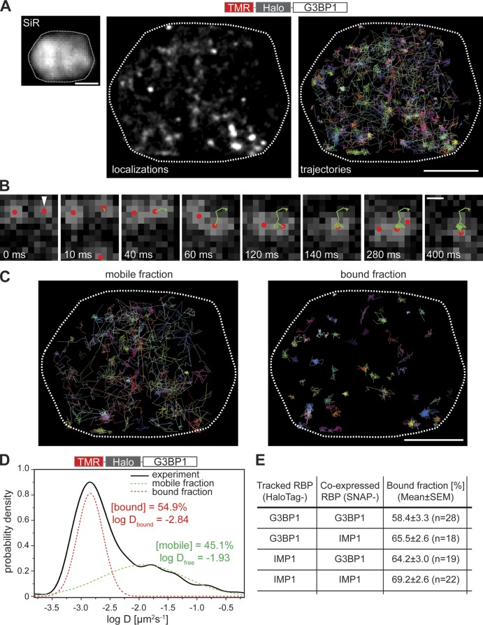
Figure 5.
G3BP1 and IMP1 exhibit a biphasic partition in a bound and mobile fraction within SGs. (A) Example of a representative granule in a double-transfected cell. The granule was identified based on SiR sta...
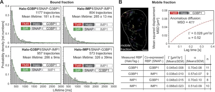
Figure 6.
G3BP1 and IMP1 have a short lifetime in the bound fraction and display anomalous subdiffusion in the mobile fraction. (A) Lifetime determination of different combinations of HaloTag- and SNAP-tagged G...
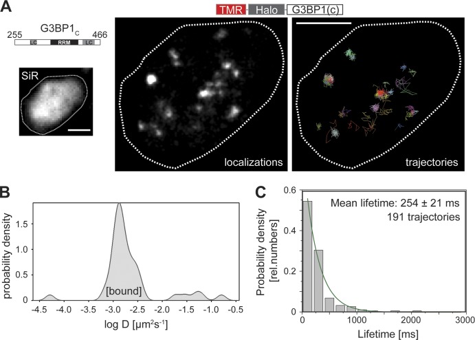
Figure 7.
Reduction in the number of LC regions of G3BP1 results in less detectable mobile molecules within the liquid phase without changing binding properties to nanocores. (A) Example of a representative gra...
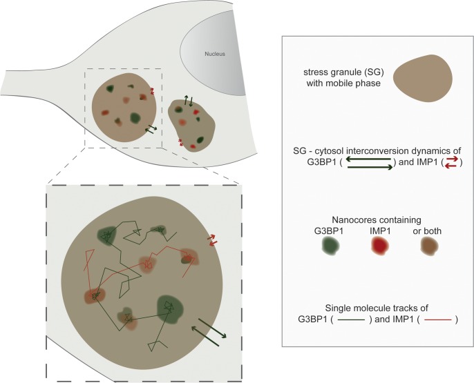
Figure 8.
Schematic representation visualizing the major findings of the study. The study reveals the presence of distributed nanocores within the mobile, liquid droplet-like phase of SGs. The two RBPs, G3BP1 (...
Figure images are served from the NIH/NLM PubMed Central Open Access Subset or Europe PMC; copyright remains with the publishers and authors.
💬 Discussion
0 commentsNo comments yet. Be the first to start a discussion!
Leave a Comment