Abstract
AbstractQuantitative phase imaging has gained popularity in bioimaging because it can avoid the need for cell staining, which, in some cases, is difficult or impossible. However, as a result, quantitative phase imaging does not provide the labelling of various specific intracellular structures. Here we show a novel computational segmentation method based on statistical inference that makes it possible for quantitative phase imaging techniques to identify the cell nucleus. We demonstrate the approach with refractive index tomograms of stain-free cells reconstructed using tomographic phase microscopy in the flow cytometry mode. In particular, by means of numerical simulations and two cancer cell lines, we demonstrate that the nucleus can be accurately distinguished within the stain-free tomograms. We show that our experimental results are consistent with confocal fluorescence microscopy data and microfluidic cyto-fluorimeter outputs. This is a remarkable step towards directly extracting specific three-dimensional intracellular structures from the phase contrast data in a typical flow cytometry configuration.
🔬 Techniques
✨ Fluorophores
🧪 Sample Preparation
🔬 Cell Lines
🏭 Microscope Brands
🧪 Reagent Suppliers
📷 Detectors
🏛️ Research Organizations (ROR)
Affiliated research institutions:
📋 Methods
Description and assessment of the CSSI method
To reconstruct the 3D RI distribution at the single-cell level in-flow, the TPM system in flow cytometry condition sketched in Fig. 2a has been employed, which is described in the Methods section along with the numerical processing summarized in Fig. 2b . Since the sub-cellular structures (i.e. organelles) often cannot be detected within the tomogram by conventional RI-based thresholding methods, the CSSI algorithm is proposed to identify the nuclear OCH. To validate the CSSI method, we preliminarily tested and assessed it on a 3D numerical cell phantom simulation, modelled with the cell membrane, nucleus, cytoplasm, and mitochondria, as shown in Fig. 3a (see the Methods section ). As reported by the histogram in Fig. 3b , a RI distribution has been assigned to each of the four sub-cellular structures. This 3D numerical cell phantom has been used to assess our CSSI algorithm for nucleus segmentation. However, nucleus segmentation is only one case of a more general technique which in principle can segment any kind of subcellular structure with a suitable spatial resolution, because it only exploits the hypothesis of knowing the location of a group of voxels belonging to the organelle to be segmented, considered as the initial reference set. In fact, the CSSI method is based on the Wilcoxon–Mann–Whitney (WMW) test 35 , 36 , that is a statistical test we use to reject or not the hypothesis for which a test set has been drawn from the same distribution as the designed reference set. In particular, the steps depicted in the scheme in Fig. 3c are performed as follows Rough clustering of the organelle voxels, exploiting the WMW test to infer the statistical similarity between different voxel clouds (i.e. the test sets) and a certain voxel cloud (i.e. the initial reference set) which contains the voxels supposed to belong to the organelle of interest. Filtering of the outlier organelle voxels when they are too far away from the centroid of the rough organelle cluster in terms of both geometric and statistical distances. Refinement of the filtered organelle cluster to improve its external shape by adding/removing smaller voxel clouds. Filling of the holes and smoothing of the corners of the refined organelle cluster by common morphological operators. Notice that, whenever the WMW test is used, the reference set is randomly selected from the last estimation of the organelle cluster until that moment, to match its dimensionality with that of the test set, thus preserving the fairness of the statistical test. Due to this random selection, by repeating several times the described steps, at each iteration j = 1,2, …, K we can obtain a slightly different estimation of the OCH. The output of each iteration is a binary valued 3D volume whose non-null values correspond to the voxels associated with the organelle. Therefore, the sum of all the K outputs provides a tomogram of occurrences, from which the probability that a voxel belongs to the organelle can be inferred through a normalization operation. Finally, the OCH is identified by a suitable probability threshold. A detailed description of the CSSI algorithm is reported in Section S1, Figs. S1,S2, and Table S1 in the Supplementary Information. In this paper we focus on the problem of stain-free nucleus segmentation, therefore we associate the initial reference set to the central voxels of the cell. Indeed, for many kinds of suspended cells, the central voxels belong to the nucleus. This property occurs especially in the case of cancer cells. This is confirmed by the 2D images of the neuroblastoma cells recorded through a FM cyto-fluorimeter (see Fig. S3 ), by the 3D morphological parameters reported in the literature for MCF-7 cells imaged through a confocal microscope 37 , and more generally by the increase of the nucleus-cytoplasm ratio demonstrated in cancer cells 38 – 42 . On the left in Fig. 3d , the sole simulated nucleus is reported in red within the blue cell shell, while on the right we show the nucleus segmented from the 3D numerical cell phantom through the CSSI algorithm. The visual comparison in Fig. 3d suggests that the proposed CSSI method allows segmenting a nucleus region very close to the original one, as also confirmed by the great quantitative performances reported below the tomograms. Moreover, to numerically assess the proposed 3D CSSI algorithm, it has been applied to reconstruct the nuclei of 1000 numerical cell phantoms simulated by randomly drawing their morphological and RI parameters from the distributions described in the Methods section and in Table S2 . The overall CSSI performances are summarized in the first column of Table S3 by means of 9 metrics, which corresponding histograms are displayed in blue in Fig. S4 . It is worth underlying that, in order to simplify the description of the CSSI algorithm and highlight its results about the stain-free nucleus identification, so far we neglected the presence of the nucleolus within the 3D numerical cell phantoms. The extended analysis with the simulation of the nucleolus reported in Section S2 and Figs. S4,S5 in the Supplementary Information highlights that the presence of nucleoli inside the nucleus does not substantially deteriorate the performances of the CSSI nucleus segmentation algorithm (see the second column of Table S3 and the corresponding orange histograms in Fig. S4 ). For example, the accuracy passes from an average value of ACC = 96.28 % in the case without the nucleolus to an average value of ACC = 95.86 % in the case with nucleolus.
Show full methods section
Description and assessment of the CSSI method
To reconstruct the 3D RI distribution at the single-cell level in-flow, the TPM system in flow cytometry condition sketched in Fig. 2a has been employed, which is described in the Methods section along with the numerical processing summarized in Fig. 2b . Since the sub-cellular structures (i.e. organelles) often cannot be detected within the tomogram by conventional RI-based thresholding methods, the CSSI algorithm is proposed to identify the nuclear OCH. To validate the CSSI method, we preliminarily tested and assessed it on a 3D numerical cell phantom simulation, modelled with the cell membrane, nucleus, cytoplasm, and mitochondria, as shown in Fig. 3a (see the Methods section ). As reported by the histogram in Fig. 3b , a RI distribution has been assigned to each of the four sub-cellular structures. This 3D numerical cell phantom has been used to assess our CSSI algorithm for nucleus segmentation. However, nucleus segmentation is only one case of a more general technique which in principle can segment any kind of subcellular structure with a suitable spatial resolution, because it only exploits the hypothesis of knowing the location of a group of voxels belonging to the organelle to be segmented, considered as the initial reference set. In fact, the CSSI method is based on the Wilcoxon–Mann–Whitney (WMW) test 35 , 36 , that is a statistical test we use to reject or not the hypothesis for which a test set has been drawn from the same distribution as the designed reference set. In particular, the steps depicted in the scheme in Fig. 3c are performed as follows Rough clustering of the organelle voxels, exploiting the WMW test to infer the statistical similarity between different voxel clouds (i.e. the test sets) and a certain voxel cloud (i.e. the initial reference set) which contains the voxels supposed to belong to the organelle of interest. Filtering of the outlier organelle voxels when they are too far away from the centroid of the rough organelle cluster in terms of both geometric and statistical distances. Refinement of the filtered organelle cluster to improve its external shape by adding/removing smaller voxel clouds. Filling of the holes and smoothing of the corners of the refined organelle cluster by common morphological operators. Notice that, whenever the WMW test is used, the reference set is randomly selected from the last estimation of the organelle cluster until that moment, to match its dimensionality with that of the test set, thus preserving the fairness of the statistical test. Due to this random selection, by repeating several times the described steps, at each iteration j = 1,2, …, K we can obtain a slightly different estimation of the OCH. The output of each iteration is a binary valued 3D volume whose non-null values correspond to the voxels associated with the organelle. Therefore, the sum of all the K outputs provides a tomogram of occurrences, from which the probability that a voxel belongs to the organelle can be inferred through a normalization operation. Finally, the OCH is identified by a suitable probability threshold. A detailed description of the CSSI algorithm is reported in Section S1, Figs. S1,S2, and Table S1 in the Supplementary Information. In this paper we focus on the problem of stain-free nucleus segmentation, therefore we associate the initial reference set to the central voxels of the cell. Indeed, for many kinds of suspended cells, the central voxels belong to the nucleus. This property occurs especially in the case of cancer cells. This is confirmed by the 2D images of the neuroblastoma cells recorded through a FM cyto-fluorimeter (see Fig. S3 ), by the 3D morphological parameters reported in the literature for MCF-7 cells imaged through a confocal microscope 37 , and more generally by the increase of the nucleus-cytoplasm ratio demonstrated in cancer cells 38 – 42 . On the left in Fig. 3d , the sole simulated nucleus is reported in red within the blue cell shell, while on the right we show the nucleus segmented from the 3D numerical cell phantom through the CSSI algorithm. The visual comparison in Fig. 3d suggests that the proposed CSSI method allows segmenting a nucleus region very close to the original one, as also confirmed by the great quantitative performances reported below the tomograms. Moreover, to numerically assess the proposed 3D CSSI algorithm, it has been applied to reconstruct the nuclei of 1000 numerical cell phantoms simulated by randomly drawing their morphological and RI parameters from the distributions described in the Methods section and in Table S2 . The overall CSSI performances are summarized in the first column of Table S3 by means of 9 metrics, which corresponding histograms are displayed in blue in Fig. S4 . It is worth underlying that, in order to simplify the description of the CSSI algorithm and highlight its results about the stain-free nucleus identification, so far we neglected the presence of the nucleolus within the 3D numerical cell phantoms. The extended analysis with the simulation of the nucleolus reported in Section S2 and Figs. S4,S5 in the Supplementary Information highlights that the presence of nucleoli inside the nucleus does not substantially deteriorate the performances of the CSSI nucleus segmentation algorithm (see the second column of Table S3 and the corresponding orange histograms in Fig. S4 ). For example, the accuracy passes from an average value of ACC = 96.28 % in the case without the nucleolus to an average value of ACC = 95.86 % in the case with nucleolus.
Experimental consistency with 2D FM cyto-fluorimetry
The proposed CSSI method has been used to retrieve the 3D nuclear OCHs from five stain-free human neuroblastoma cancer cells (SK-N-SH cell line), reconstructed by TPM in flow cytometry. The isolevels representation of an SK-N-SH cell is shown in Fig. 4a , highlighting in red the 3D segmented nuclear OCH within the blue cell shell. Moreover, its central slice is displayed in Fig. 4b , in which the segmented nucleus is marked by the red line, while in Fig. 4c we report in green the corresponding 3D RI histogram, separating in red and in blue the contributions of the 3D nuclear OCH and the 3D non-nucleus region, respectively. To experimentally assess the 3D segmentation technique, we digitally projected the segmented 3D TPM reconstruction back to 2D where the experimental 2D FM images are available for comparison. In particular, the segmented RI tomogram is digitally rotated from 0° to 150° with 30° angular step around x -, y -, and z -axes, and then its silhouettes along the z -, x -, and y -axes, respectively, are considered to create 2D TPM segmented projections, as sketched in Fig. 4a . According to the ray optics approximation, the phase measured by digital holography (DH) is directly proportional to the integral of the RI values along the direction perpendicular to the plane of the camera. In this way, 18 unlabelled QPMs were obtained. As shown in a re-projected QPM on the left in Fig. 4d , it is cumbersome to recognize a sub-cellular structuring since no label is employed. However, thanks to the proposed 3D CSSI algorithm, the region occupied by the nucleus can be also marked (red line) in the 2D TPM projection within the outer cell (blue line). We exploit this process to further assess the proposed segmentation algorithm, by comparing the 3D results obtained through the in-flow TPM technique with a conventional 2D FM cyto-fluorimeter (i.e. ImageStreamX, see the Methods section ). The latter has been used to record 11549 2D FM images of flowing SK-N-SH single cells, in which the nuclei have been stained through fluorescent dyes. On the right in Fig. 4d , the bright-field image of an SK-N-SH cell has been combined with the corresponding fluorescent image of the marked nucleus, therefore the false-color visualization makes the nucleus easily distinguishable (red line) with respect to the outer cell (blue line). ImagesStreamX can record a single random 2D image for each cell since it goes through the field of view (FOV) once. Instead, TPM allows the 3D tomographic reconstruction of a single cell. Through the reprojection process, we simulate the transition of the reconstructed cell within the ImageStreamX FOV at different 18 3D orientations with respect to the optical axis. In this way, we digitally replicate the ImageStreamX recording process and we also increase the dataset of 2D TPM images avoiding a high correlation between the reprojections of the same cell, thanks to the choice of a big angular step (i.e., 30°). Hence, in the 3D scatter plot in Fig. 4e , we quantitively compare some 2D morphological parameters representative of nucleus size, nucleus shape, and nucleus position, i.e. nucleus-cell area ratio (NCAR), nucleus aspect ratio (NAR), and normalized nucleus-cell centroid distance (NNCCD), respectively, measured from both 90 TPM images (red dots) and 11549 FM images (blue dots). In particular, we computed the NAR as the ratio between the minor axis and the major axis of the best-fitted ellipse to the nucleus surface, while the nucleus-cell centroid distance refers to 2D centroids and has been normalized to the radius of a circle having the same area of the cell, thus obtaining NNCCD. The 3D scatter plot highlights the very good agreement between TPM and FM 2D nuclear features since the TPM red dots are completely contained within the FM blue cloud. In addition, by using the one-sample multivariate Hotelling's T 2 test 43 between TPM and FM measurements about NCAR, NAR, and NNCCD, we also obtained a high p-value, i.e. 0.962, according to which it is not rejected with high confidence level the hypothesis that TPM and FM 2D nuclear features have been drawn from the same distributions. This quantitative comparison is summarized in Table S4 . Moreover, to better visualize the 3D scatter plot in Fig. 4e , we split it into three different 2D scatter plots, shown in Figs. 4f-h .
Experimental consistency with 3D FM confocal microscope
For the second experimental assessment, three stain-free human breast cancer cells (MCF-7 cells) have been reconstructed by TPM in flow cytometry and then segmented by the CSSI method, as shown in the example in Figs. 5a,b . In particular, the nucleus shell is marked in red within the blue cell shell in the isolevels representation of Fig. 5a , which segmented central slice is displayed in Fig. 5b . Moreover, in Fig. 5c , we display in green its 3D RI histogram, also separating the RI distribution of the 3D nuclear OCH (red) and the 3D non-nucleus region (blue). In this case, the experimental assessment is based on a quantitative comparison with the 3D morphological parameters measured in ref. 37, in which a confocal microscope has been employed to find differences between viable and apoptotic MCF-7 cells through 3D morphological features extraction. In this study, 206 suspended cells were stained with three fluorescent dyes to measure average values and standard deviations of 3D morphological parameters about the overall cell and its nucleus and mitochondria. A synthetic description of 3D nucleus size, shape, and position is given by nucleus-cell volume ratio (NCVR), nucleus surface-volume ratio (NSVR), and normalized nucleus-cell centroid distance (NNCCD), respectively. In particular, in this case, the nucleus-cell centroid distance refers to 3D centroids and has been normalized with respect to the radius of a sphere having the same cell volume, thus obtaining NNCCD. Moreover, it is worth underlining that NCVR and NSVR are direct measurements reported in ref. 37, while NNCCD is an indirect measurement since it has been computed by using the direct ones in ref. 37. In the 2D scatter plots in Figs. 5d-f regarding nucleus size, shape, and position, the three TPM measurements (red dots) are reported along with three blue rectangles, which are the intervals μ ± 1 σ , μ ± 2 σ , and μ ± 3 σ , with μ the average value and σ the standard deviation of the same parameters measured by FM confocal microscope. These scatter plots highlight a very good agreement between the 3D nucleus identified in labelled static MCF-7 cells by confocal microscope and the 3D nucleus segmented in unlabelled flowing MCF-7 cells by the proposed CSSI algorithm. In fact, all the TPM values are located in the 1σ-interval around the FM average values, except for shape measurement, that is anyway located in the 2σ-interval around the FM average value ( Figs. 5d,f ). The values shown in Figs. 5d-f are summarized in Table S5 .
Methods Sample preparation
The human breast cancer cells (MCF-7 cell line) and the human neuroblastoma cells (SK-N-SH cell line) were selected for tomographic experiments. The MCF-7 and the SK-N-SH cells were cultured in RPMI 1640 and in Minimum Essential Medium Eagle (MEM) from Sigma Aldrich, respectively. Both cell culture media were supplemented with 10% fetal bovine serum, 2 mM L-glutamine, 100 μg ml −1 streptomycin, and 100 U ml −1 penicillin. Then, cells were collected from the Petri dish by incubation for 5 min with a 0.05% trypsin–EDTA solution (Sigma, St. Louis, MO). Finally, the MCF-7 and the SK-N-SH cells were centrifuged for 5 min at 125 x g, resuspended in complete medium, and injected into the microfluidic channel for the TPM experiment in flow cytometry condition. The SK-N-SH cells were also analysed through a FM cyto-fluorimeter. To this aim, 7 million SK-N-SH cells were resuspended in Phosphate Buffered Saline (PBS), 1X (Sigma) and exposed to 25 μM DRAQ5 Fluorescent Probe for 5 min at room temperature under agitation (#62254, Thermo Scientific™). Tomographic phase microscopy setup in flow cytometry condition In a QPM, phase-contrast is due to the optical path length difference between the unlabelled biological specimen and its background because of the combination of its thickness and its RI 2 . These two quantities can be decoupled by recording multiple 2D QPMs at different viewing angles around the sample, thus performing the 3D TPM. However, unlike conventional TPM methods, in our setup the DH microscope acquires multiple digital holograms of flowing and rotating cells within a microfluidic channel, exploiting the hydrodynamic forces produced by a laminar flow 30 , 31 . In fact, the light beam generated by the laser (Laser Quantum – Torus, emitting at a wavelength λ = 532 nm) is coupled into an optical fibre, which splits it into an object beam and a reference beam in order to constitute a Mach−Zehnder interferometer in off-axis configuration. The object beam exits from the fibre and is collimated to probe the biological sample that flows at 7 nL/s along a commercial microfluidic channel with cross section 200 μm × 200 μm (Microfluidic Chip-Shop). The flux velocity is controlled by a pumping system (CETONI – neMESYS) that ensures temporal stability of the parabolic velocity profile into the microchannel. The wavefield passing throughout the sample is collected by the Microscope Objective (Zeiss 40× – oil immersion – 1.3 numerical aperture) and directed to the 2048 × 2048 CMOS camera (USB 3.0 U-eye, from IDS) by means of a Beam-Splitter that allows the interference with the reference beam. The interference patterns of the single cells rotating into a 170 μm × 170 μm FOV are recorded at 35 fps. The proposed TPM system in flow cytometry has the advantage to work in label-free modality, so the sample preparation time related to the nucleus staining is completely skipped. Instead, the experiment to acquire 1000 cells can take 30-60 minutes, since tens of images per cell must be recorded to retrieve their 3D tomographic reconstruction. The described opto-fluidic setting is able to provide potentially a throughput of about 100 cells/minute. It is important to underline that the maximum throughput achievable by a tomographic system of rotating cells in continuous flow is theoretically much lower than the conventional imaging flow cytometer. In fact, in order to retrieve the tomographic data, one needs to collect from tens to hundreds images per cell instead of a single snapshot. This automatically reduces the throughput of the in-flow TPM system by one or two orders of magnitude with respect to the conventional imaging flow cytometer. On the other hand, our system does not need the cells to be in microfluidic focusing, thus multiple cells can be simultaneous imaged within the same FOV (e.g. by using a larger camera sensor and/or by increasing the cell concentration) in order to increase the throughput. Moreover, also the flow rate can be increased over 7 nL/sec but with the constraint to avoid cell deformations and to guarantee that a full cell rotation occurs within the imaged FOV. Finally, it is possible to use multiple parallel microfluidic channels on the same chip, proportionally increasing the throughput. Actually, some of these opto-fluidics solutions to increase the throughput have been exploited in our very recent work 50 . According to the reference system sketched in Fig. 2a , cells flow along the y-axis and continuously rotate around the x-axis thanks to the microfluidic properties 51 , while their holograms are recorded along the z-axis. Then, as summarized in Fig. 2b , numerical operations are performed to reconstruct the stain-free 3D RI tomograms of the recorded flowing single-cells. The off-axis configuration allows demodulating each hologram of the recorded sequence by filtering the real diffraction order 52 . Then, the 3D positions of the flowing cells within the microfluidic channel are computed through a holographic tracking algorithm 53 . Each demodulated hologram is numerically propagated along the z-axis through the Angular Spectrum formula 52 in order to minimize a contrast-based metric, i.e. the Tamura Coefficient 53 (TC), to recover the z-position of the cell and refocus it. The QPMs are then obtained by implementing the phase unwrapping algorithm 52 on the corresponding refocused complex wavefronts. In each QPM, the weighted centroids provide the xy -positions of the cell, which are used to center it in its cropped region of interest (ROI), as shown in Fig. 4d , thus avoiding motion artefacts in the final 3D tomogram. Moreover, the microfluidic properties and the high frame rate allow to linearize the relationship between the angular and the translational speeds 51 . Therefore, the K unknown rolling angles ϑ K are estimated by using the computed y -positions as follows (1) ϑ k = 180 ∘ y k − y 1 y f 180 − y 1 , where K = 1, …, K is the frame index. The f 180 value is the index of the frame at which the cell has rotated of 180° with respect to the first frame of the sequence. It is computed by minimizing the Tamura Similarity Index (TSI), that is a phase image similarity metric based on the evaluation of the local contrast calculated on all the QPMs of the rolling cell though the TC. The tomographic reconstruction is firstly obtained by the inverse Radon transform, and it is then enhanced though the LT algorithm.
Learning Tomography algorithm
LT is an iterative reconstruction algorithm based on a nonlinear forward model, beam propagation method (BPM), to capture high orders of scattering 29 . Using the BPM, we propagate an incident light illumination on an initial guess acquired by the inverse Radon transform and compare the resulting field with the experimentally recorded field. The error between the two fields is backpropagated to calculate the gradient 54 . At each iteration of LT, the gradient calculation is repeated for 8 randomly selected rotation angles, and the corresponding gradients are rotated and summed to update the current solution. As an intermediate step, the total variation regularization was employed. The total iteration number is 200 with a step size of 0.00025 and a regularization parameter of 0.005. In order to run LT, we need two electric fields, incident and total electric fields. The amplitude of the incident field was estimated from the amplitude of the total electric field by low-pass filtering in the Fourier domain with a circular aperture whose radius is 0.176 k 0 , where k 0 = 2 π λ given a wavelength λ = 532 nm in a vacuum. In other words, we assume that the high-frequency information in the amplitude of the total electric field was only attributed to the light interference caused by a sample when illuminated by an illumination with slowly varying amplitude. FM cyto-fluorimeter In order to record thousands of 2D FM images, a commercial multispectral flow cyto-fluorimeter has been employed, i.e., Amnis ImageStreamX®. Cells are hydrodynamically focused within a micro-channel, and then they are probed both by a transversal brightfield light source and by orthogonal lasers. The fluorescence emissions and the light scattered and transmitted from the cells are collected by an objective lens. After passing through a spectral decomposition element, the collected light is divided into multiple beams at different angles according to their spectral bands. The separated light beams propagate up to 6 different physical locations of one of the two CCD cameras (256 rows of pixels), which operates in time operation. Therefore, the image of each single flowing cell is decomposed into 6 separate sub-images on each of the two CCD cameras, based on their spectral band, thus allowing the simultaneous acquisition of up to 12 images of the same cell, including brightfield, scatter, and multiple fluorescent images. Hence, Amnis ImageStreamX® combines the single-cell analysis of the standard FM microscopy with the statistical significance due to large number of samples provided by standard flow-cytometry. ImageStreamX Mark II Flow Cytometer (Luminex Corporation) was used to acquire 11549 single cells images at 60× magnification. For each single cell, we recorded two simultaneous images, i.e., a brightfield image of the flowing cell and its corresponding FM image. To segment nucleus, we analysed the single cells using the IDEAS software (version 6.2.64.0), which combines fluorescence intensity (DRAQ5) and morphometric measures (darkfield), generating a global threshold of the FM signal corresponding to the nucleus size. The automatic calibration provided by the instrument, corresponding to 0.33 μm/pixel, was employed to measure 2D morphological parameters related to the cell and the nucleus, in order to realize a quantitative comparison with the tomographic reconstructions. Three of the recorded brightfield and fluorescent images are shown at the top and at the bottom of Fig. S3 , respectively, with overlapped in red the contour of the segmented nuclei. In the FM cyto-fluorimeter experiments, the sample preparation step takes ~ 45 minutes, consisting of adding a specific stain (DRAQ5) to label nuclei, while the experiment to collect 1000 images (one per cell) takes at least 5 minutes. 3D numerical cell phantom In ref. 37 , a confocal microscope has been employed to find differences between viable and apoptotic MCF-7 cells through 3D morphological features extraction. In particular, 206 cells were stained with three fluorescent dyes in order to measure the average value and standard deviation of 3D morphological parameters about the overall cell and its nucleus and mitochondria. We exploit these measurements to simulate a 3D numerical cell phantom, by setting 1 px = 0.12 μm. It is made of four sub-cellular structures, i.e., cell membrane, cytoplasm, nucleus, and mitochondria. We shape cell, nucleus, and mitochondria as ellipsoids, then we make irregular the cell external surface, and finally we obtain cytoplasm through a morphological erosion of the cell shape. Moreover, in each simulation, the number of mitochondria is drawn from the uniform distribution U 1 { a 1 , b 1 }. A 3D numerical cell phantom is displayed in Fig. 3a , in which 18 mitochondria have been simulated. To each simulated 3D sub-cellular component, we assign a RI distribution, as shown by the RI histogram in Fig. 3b . Measuring accurate RI values at sub-cellular level is still a deeply debated topic 55 , 56 . Hence, we cannot replicate realistic RIs since they are not yet well known, therefore we simulate the unfavourable case for our testing purpose segmenting the nucleus from cytoplasm, i.e., we model overlapped subcellular distributions of the RI values. In particular, for each cell membrane voxel, we draw its RI from distribution N 1 ( μ 1 , σ 2 ). Instead, without knowing if the nucleus RIs are greater than the cytoplasm ones or vice versa, in each simulation we randomly assign cytoplasm and nucleus to distributions N 2 ( μ 2 , σ 2 ) or N 3 ( μ 3 , σ 2 ). It is worth remarking that, to strengthen the numerical assessment, we increase the randomness of the RI assignments among the different simulations, because each voxel belonging to cell membrane, nucleus, and cytoplasm is drawn from gaussian distributions N 1 , N 2 , and N 3 (or N 1 , N 3 , and N 2 ), respectively, which average values μ 1 , μ 2 , and μ 3 are in turn drawn from other gaussian distributions for each voxel extraction, i.e. N μ 1 ( μ μ 1 , σ μ 2 ) , N μ 2 ( μ μ 2 , σ μ 2 ) and N μ 3 ( μ μ 3 , σ μ 2 ) , respectively. Instead, as regards mitochondria, each of them has a RI gaussian distribution N 4 ( μ 4 , σ 2 ) which average value μ 4 is drawn from the gaussian distribution N μ 4 ( μ μ 4 , N μ 4 ( μ μ 4 , σ μ 2 ) ) for each mitochondrion and not for each voxel. Moreover, we create a RI transition zone straddling the nucleus to cytoplasm, thus avoiding any discontinuity that could somehow facilitate the segmentation. In particular, after drawing all nucleus and cytoplasm values, RIs that are in the middle of their average values are assigned to the voxels of the transition zone, as highlighted by the red arrow at the top of Fig. 3b . This transition zone is obtained through morphological erosion and dilation of the nucleus ellipsoid, by using a spherical structuring element, which radius is drawn from the uniform distribution U 2 { a 2 , b 2 } px for each simulation, thus resulting in an internal nucleus volume that is about 85-95 % of the total nucleus volume. In the example in Figs. 3a,b , a 3 px radius has been selected. All the described parameters are reported in Table S2 .
Supplementary Material Supplementary Information Supplementary Video 1 Supplementary Video 2
📊 Figures
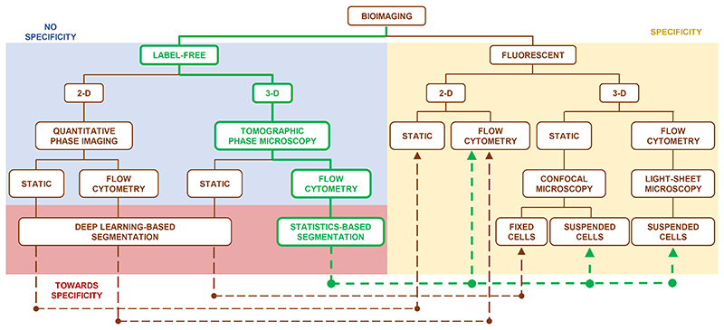
Fig. 1
Comparison between label-free and fluorescent bioimaging in microscopy.
Unlike the label-free bioimaging (blue box), the fluorescent bioimaging (yellow box) has sub-cellular specificity because nucleus is marked, but it is qualitative and limited by the staining itself. T...

Fig. 2
TPM in flow cytometry technique.
a Sketch of the in-flow TPM setup based on a digital holographic microscope in off-axis configuration. BSF, Beam Splitter Fiber; MP, Microfluidic Pump; MC, Microfluidic Channel; OB, Object Beam; MO, M...

Fig. 3
Numerical assessment of the CSSI algorithm applied to segment the 3D nuclear OCH from a 3D numerical cell phantom ( Supplementary Video 1 ).
a Isolevels representation of the 3D cell model, simulated with four sub-cellular components, i.e., cell membrane, cytoplasm, nucleus, and 18 mitochondria. b Histogram of the RI values assigned to eac...

Fig. 4
Experimental assessment of the CSSI algorithm applied to segment the 3D nuclear OCHs from unlabelled in-flow TPM reconstructions of five SK-N-SH cells, by comparison with the morphological parameters measured through a 2D FM cyto-fluorimeter ( Supplementary Video 2 ).
a 3D segmented nucleus (red) within the 3D cell shell (blue) of an SK-N-SH cell reconstructed by TPM. The segmented tomogram is rotated around the x -, y -, and z -axes (orange arrows) and then reproj...

Fig. 5
Experimental assessment of the CSSI algorithm applied to segment the 3D nuclear OCHs from unlabelled in-flow TPM reconstructions of three MCF-7 cells, by comparison with the morphological parameters measured through a 3D FM confocal microscope ( Supplementary Video 2 ).
a 3D segmented nuclear OCH (red) within unlabelled 3D cell shell (blue) reconstructed through in-flow TPM. b Central slice of the isolevels representation in (a), with nucleus marked by the red line. ...
Figure images are served from the NIH/NLM PubMed Central Open Access Subset or Europe PMC; copyright remains with the publishers and authors.
💬 Discussion
0 commentsNo comments yet. Be the first to start a discussion!
Leave a Comment