Abstract
Abstract Mechanical forces acting on ligand-engaged T-cell receptors (TCRs) have previously been implicated in T-cell antigen recognition, yet their magnitude, spread, and temporal behavior are still poorly defined. We here report a FRET-based sensor equipped either with a TCR-reactive single chain antibody fragment or peptide-loaded MHC, the physiological TCR-ligand. The sensor was tethered to planar glass-supported lipid bilayers (SLBs) and informed most directly on the magnitude and kinetics of TCR-imposed forces at the single molecule level. When confronting T-cells with gel-phase SLBs we observed both prior and upon T-cell activation a single, well-resolvable force-peak of approximately 5 pN and force loading rates on the TCR of 1.5 pN per second. When facing fluid-phase SLBs instead, T-cells still exerted tensile forces yet of threefold reduced magnitude and only prior to but not upon activation.
🔬 Techniques
🔭 Microscopes
🧬 Organisms
💻 Software
✨ Fluorophores
🧪 Sample Preparation
🔬 Cell Lines
🏭 Microscope Brands
🧪 Reagent Suppliers
🔴 Lasers
📷 Detectors
🎨 Filters
💻 Software Details
💾 Data Repositories
🏛️ Research Organizations (ROR)
Affiliated research institutions:
📋 Methods
Force sensor—anchor unit Recombinant mSAv-3xHis 6 served as anchor unit for the force sensor and was produced as described 33 . Briefly, biotin binding deficient subunits equipped with a C-terminal His 6 -tag—“dead”—and functional subunits with C-terminal 3C protease cleaving site followed by Glu 6 -tag—“alive”—were expressed as inclusion bodies in E. coli BL-21 using the pET expression system (Novagen). Inclusion bodies were dissolved in 6 M guanidine hydrochloride at 10 mg/ml, mixed at a ratio of 3 “dead” to 1 “alive” subunit and refolded in 100 volumes PBS. The salt concentration was reduced to 2 mM by cycles of concentration using a 10 kDa cutoff spin concentrator (Amicon) and dilution with 20 mM Tris pH 7.0. The mixture was loaded onto a MonoQ 5/50 column (GE Healthcare), and after washing the column with 100 mM NaCl in 20 mM Tris pH 7.0 mSAv-3xHis 6 was eluted at 20 mM Tris pH 7.0, 240 mM NaCl. Human 3 C protease (Pierce) was added and allowed to cleave the Glu 6 -tag overnight. The digested protein was subjected to Superdex 200 (GE Healthcare) size exclusion chromatography in PBS to yield to pure anchor unit. Force sensor—spring unit The MFS peptide biotin-N-GG C GS(GPGGA) 5 GG K YGGS-K(ε-N 3 ) (residues for fluorophore attachment are underlined), MFS C peptide biotin-N-GGGGS(GPGGA) 5 GG K Y C GS-K(ε-N 3 ) and the MFS 0 peptide biotin-N-GGGGS (GPGGA) 5 GGKYG GS-K(ε-N 3 ) were purified via preparative C18 reverse phase HPLC (5 µm particle size, 250 × 21.2 mm, Agilent) applying a linear gradient of 0.1% triflouracetic acid (TFA) in deionized water (buffer A) and 0.1% TFA, 9.9% deionized water, 90% acetonitrile (buffer B) over 80 min at a flow rate of 5 ml/min. The identity of the spring modules was confirmed via MALDI-TOF mass spectrometry (Bruker). 350 µg lyophilized peptide was dissolved in PBS at a final concentration of 5 mg/ml, mixed with Alexa Fluor 555 maleimide (Thermo Fisher Scientific) at a 1.5-fold molar surplus and then incubated for 2 h followed by an incubation with 1.5-fold excess Alexa Fluor 647 succinimidyl ester (Thermo Fisher Scientific) in the presence of 330 mM NaHCO 3 for 2 h at room temperature. HPLC purification and lyophilization was performed after each step and successful conjugation was confirmed via mass spectrometry. Force sensor—functional unit TCRβ-reactive H57 antibody single chain fragments featuring a C-terminal unpaired cysteine residue (H57 cys scF V ) were expressed in E. coli BL-21 as inclusion bodies using the pET expression system (Novagen) and refolded by multiple dialysis steps continuously diluting the concentration of guanidine hydrochloride within the refolding buffer (50 mM Tris pH = 8.0, 200 mM NaCl, 1 mM EDTA); in a final step the refolded protein was dialyzed against 1×PBS 9 , 42 . The product was then concentrated using a 10 kDa cutoff spin concentrator (Amicon) in the presence of 25 µM Tris-(2-carboxyethyl)phosphine hydrochloride (TCEP, Pierce). Monomeric H57 cys scF V was purified by Superdex 75 (GE Healthcare) size exclusion chromatography in PBS, then concentrated to 1 mg/ml in the presence of 25 µM TCEP and allowed to react with a 10-fold surplus of dibenzylcyclooctyne-maleimide (DBCO, Jena Bioscience) for 2 h at room temperature. Unreacted DBCO was removed by gel filtration and proteins were brought to a concentration of 1 mg/ml. IE k α featuring an additional C-terminal cysteine residue and IE k β were also expressed as inclusion bodies and refolded in the presence of MCC 88–103 peptide (ANERADLIAYLKQATK, Intavis) for 2 weeks 9 . Correctly folded IE k molecules were isolated via an in house built 14-4-4 antibody column, reduced with 25 µM TCEP followed by S200 gel filtration. Monomeric IE k MCC with unpaired cysteine residue was collected and coupled to DBCO as described above.
Show full methods section
Force sensor—anchor unit Recombinant mSAv-3xHis 6 served as anchor unit for the force sensor and was produced as described 33 . Briefly, biotin binding deficient subunits equipped with a C-terminal His 6 -tag—“dead”—and functional subunits with C-terminal 3C protease cleaving site followed by Glu 6 -tag—“alive”—were expressed as inclusion bodies in E. coli BL-21 using the pET expression system (Novagen). Inclusion bodies were dissolved in 6 M guanidine hydrochloride at 10 mg/ml, mixed at a ratio of 3 “dead” to 1 “alive” subunit and refolded in 100 volumes PBS. The salt concentration was reduced to 2 mM by cycles of concentration using a 10 kDa cutoff spin concentrator (Amicon) and dilution with 20 mM Tris pH 7.0. The mixture was loaded onto a MonoQ 5/50 column (GE Healthcare), and after washing the column with 100 mM NaCl in 20 mM Tris pH 7.0 mSAv-3xHis 6 was eluted at 20 mM Tris pH 7.0, 240 mM NaCl. Human 3 C protease (Pierce) was added and allowed to cleave the Glu 6 -tag overnight. The digested protein was subjected to Superdex 200 (GE Healthcare) size exclusion chromatography in PBS to yield to pure anchor unit. Force sensor—spring unit The MFS peptide biotin-N-GG C GS(GPGGA) 5 GG K YGGS-K(ε-N 3 ) (residues for fluorophore attachment are underlined), MFS C peptide biotin-N-GGGGS(GPGGA) 5 GG K Y C GS-K(ε-N 3 ) and the MFS 0 peptide biotin-N-GGGGS (GPGGA) 5 GGKYG GS-K(ε-N 3 ) were purified via preparative C18 reverse phase HPLC (5 µm particle size, 250 × 21.2 mm, Agilent) applying a linear gradient of 0.1% triflouracetic acid (TFA) in deionized water (buffer A) and 0.1% TFA, 9.9% deionized water, 90% acetonitrile (buffer B) over 80 min at a flow rate of 5 ml/min. The identity of the spring modules was confirmed via MALDI-TOF mass spectrometry (Bruker). 350 µg lyophilized peptide was dissolved in PBS at a final concentration of 5 mg/ml, mixed with Alexa Fluor 555 maleimide (Thermo Fisher Scientific) at a 1.5-fold molar surplus and then incubated for 2 h followed by an incubation with 1.5-fold excess Alexa Fluor 647 succinimidyl ester (Thermo Fisher Scientific) in the presence of 330 mM NaHCO 3 for 2 h at room temperature. HPLC purification and lyophilization was performed after each step and successful conjugation was confirmed via mass spectrometry. Force sensor—functional unit TCRβ-reactive H57 antibody single chain fragments featuring a C-terminal unpaired cysteine residue (H57 cys scF V ) were expressed in E. coli BL-21 as inclusion bodies using the pET expression system (Novagen) and refolded by multiple dialysis steps continuously diluting the concentration of guanidine hydrochloride within the refolding buffer (50 mM Tris pH = 8.0, 200 mM NaCl, 1 mM EDTA); in a final step the refolded protein was dialyzed against 1×PBS 9 , 42 . The product was then concentrated using a 10 kDa cutoff spin concentrator (Amicon) in the presence of 25 µM Tris-(2-carboxyethyl)phosphine hydrochloride (TCEP, Pierce). Monomeric H57 cys scF V was purified by Superdex 75 (GE Healthcare) size exclusion chromatography in PBS, then concentrated to 1 mg/ml in the presence of 25 µM TCEP and allowed to react with a 10-fold surplus of dibenzylcyclooctyne-maleimide (DBCO, Jena Bioscience) for 2 h at room temperature. Unreacted DBCO was removed by gel filtration and proteins were brought to a concentration of 1 mg/ml. IE k α featuring an additional C-terminal cysteine residue and IE k β were also expressed as inclusion bodies and refolded in the presence of MCC 88–103 peptide (ANERADLIAYLKQATK, Intavis) for 2 weeks 9 . Correctly folded IE k molecules were isolated via an in house built 14-4-4 antibody column, reduced with 25 µM TCEP followed by S200 gel filtration. Monomeric IE k MCC with unpaired cysteine residue was collected and coupled to DBCO as described above.
Force sensor assembly
Refolded from E. coli inclusion bodies H57-scF V were modified for sensor attachment with DBCO maleimide at a mutant unpaired C-terminal cysteine residue (Supplementary Fig. 1A–D ). MFS peptides were mixed with DBCO-conjugated proteins and 25 vol% 2 M Tris pH 8.0 at a molar ratio of at least 5:1 and incubated for 2 h at room temperature. Unreacted protein was removed with the use of a monomeric avidin column (Pierce). After elution with biotin, unconjugated spring was separated from MFS conjugates using size exclusion chromatography on a Superdex 75 column (GE Healthcare). mSAv-3xHis 6 gel shift assays documented successful conjugation as only a neglectable proportion of H57-scFv gave rise to dimers (Supplementary Fig. 1E ). The existence of such entities may have yielded a small underestimation in ensemble readouts. However, in the case of single-molecule experiments, multimeric structures could be directly identified and subsequently eliminated from the analysis. T-cells Antigen-experienced 5c.c7 murine T-cell blasts were obtained as previously described 50 . Briefly, 7.5*10 6 /ml spleenocytes were stimulated with 2 µM HPLC-purified MCC peptide (ANERADLIAYLKQATK, Intavis Bioanalytical Instruments) in T-cell medium, which consisted of RPMI 1640 (Gibco) supplemented with 10% FCS (Sigma), 100 U/ml penicillin/streptomycin (Gibco), 2 mM glutamate (Gibco), 1 mM sodium pyruvate (Gibco), 1× non-essential amino acids (Gibco) and 50 µM ß-Mercaptoethanol (Gibco). Culture volume was doubled and also supplemented with 100 U/ml IL-2 (eBioscience) on day 2. T-cell cultures were expanded in a ratio of 1:1 on day 3 and 5. Dead cells were removed by centrifugation on a cushion of Histopaque-1119 (Sigma) on day 6. T-cells were used for experiments on day 7–9 after initial stimulation. OT-1 aβ TCR-transgenic mice of 8–12 weeks were sacrificed to collect spleen and lymph nodes (housing conditions: 22 °C, 53% relative humidity, 12 h dark–light cycle). Isolated splenic APCs were loaded with 1 µM C18 reverse-phase HPLC-purified Ovalbumin (Ova 257–264, SIINFEKL) peptide. After 1 h incubation, splenic APCs were washed with RPMI 1640 culture medium (Gibco). Subsequently, lymph-node-derived cells were mixed in a 1:2 ratio with OVA-peptide pulsed spleenocytes and cultured in RPMI 1640 culture medium (Gibco) supplemented with 10% fetal calf serum (FCS) (Sigma), 100 U/ml penicillin/streptomycin (Gibco), 2 mM glutamate (Gibco), 1 mM sodium pyruvate (Gibco), 1× non-essential amino acids (Gibco), and 50 µM ß-mercaptoethanol (Gibco) at 37 °C and 5% CO 2 . On day 2, IL-2 was added to a final concentration of 50 U/ml. Cells were split 1:1 with fresh media every second day (day 3, 5, and 7). Dead cells were removed on day 7 prior to splitting by Ficoll-Paque Plus (Merck) step gradient centrifugation and cytotoxic T lymphocytes (CTLs) were used on day 8–10 for experiments.
Ethical compliance statement
Mice were bred and euthanized for T-cell isolation according to guidelines and protocols evaluated by the ethics committee of the Medical University of Vienna and approved by the Federal Ministry of Science, Research and Economy, BMWFW (BMWFW-66.009/0378-WF/V/3b/2016). Animal husbandry and experimentation were performed under national laws (Federal Ministry of Science, Research and Economy, Vienna, Austria) and the ethics committee of the Medical University of Vienna and according to the guidelines of the Federation of Laboratory Animal Science Associations (FELASA).
Reagents Hank’s buffered salt solution
(HBSS) and phosphate buffered saline (PBS), Cytochalasin D (from Zygosporium masonii) as well as fetal calf serum (FCS) were from Sigma Aldrich (Merck KGaA, Germany). DPPC, 1-palmitoyl-2-oleoyl-glycero-3-phosphocholine (POPC), and 1,2-dioleoyl-sn-glycero-3-[(N-(5-amino-1-carboxypentyl)iminodiacetic acid)succinyl] (nickel salt) (Ni-NTA-DGS) were from Avanti Polar Lipids, Inc., USA. ICAM-1 and B7-1 were produced in Hi-5 insect cells using baculovirus and purified via size exclusion and ion exchange chromatography 9 . Preparation of functionalized lipid bilayers 98 mol-% POPC or DPPC and 2 mol-% Ni-NTA-DGS, all dissolved in chloroform, were mixed and then dried under nitrogen flow for 20 min. The lipid mixture was suspended in 1 ml PBS at room temperature (POPC) or 55 °C (DPPC) and then sonicated for 10 min in an ultrasound bath (USC500TH, VWR, England) at the same temperature to form small unilamellar vesicles (SUVs). The SUV solution was finally diluted to 125 μM using PBS. Cover slips (MENZEL-Gläser Deckgläser 24 × 60 mm #1.5) were treated in a plasma cleaner (PDC-002 Plasma Cleaner Harrick Plasma, Ithaca, NY, USA) for 10 min and glued to the bottom of an eight-well chamber (Nunc Lab-Tek, Thermo Scientific, USA) using duplicating silicone (Twinsil soft 18, picodent, Germany). SUVs were incubated for 20 min at room temperature (POPC) or 55 °C (DPPC) to form bilayers. After incubation, excess vesicles were washed away using PBS. His-tagged proteins (for activating conditions: 10 ng mSAv-3xHis 6 , 30 ng ICAM-1, 50 ng B7-1; for scanning conditions: 0.4 ng mSAv-3xHis 6 , 30 ng ICAM-1) were added in 0.5 ml PBS to each well and incubated for 75 min at room temperature. Afterwards, the bilayer was washed with PBS. Finally, the bilayer was incubated for 20 min with biotinylated MFS variants (for activating conditions: 10 ng MFS 0 , 5–20 pg MFS or MFS C ; for scanning conditions: 20–60 pg MFS or MFS C ) in 0.5 ml PBS per well for binding to the mSAv-3xHis 6 . Bilayers were washed again to remove excess MFS. Immediately before adding cells, the buffer was exchanged for HBSS containing 2% FCS. For ensemble experiments, molecular densities were determined by dividing the fluorescence signal per pixel by the single molecule brightness recorded at the same settings, considering the effective pixel width of 160 nm. In single molecule samples, densities were determined by counting the number of molecules and dividing by the area of the field of view. T-cell calcium imaging 3 ml of HBSS + 2% FCS were added to ~10 6 T-cells. After centrifugation (300× g for 3 min), supernatant was removed and cells were incubated with 1 μg of Fura-2 AM dye (Thermo Scientific, USA) at 1 mg/ml DMSO in a total volume of 100 µl for 20 min at room temperature, and washed (addition of 5 ml HBSS + 2% FCS, centrifugation at 300× g for 3 min, removal of supernatant, resuspension in 100 µl). Cells were kept at room temperature until seeding them onto the functionalized bilayers and for a maximal duration of 30 min. Time-lapse movies were recorded using alternating excitation (340 and 380 nm, 50 and 10 ms illumination, respectively) using a monochromatic light source (Polychrome V, TILL Photonics), coupled into a Zeiss Axiovert 200M microscope equipped with a 10× objective (UPlanFL N 10×/0.30, Olympus) and an Andor iXon Ultra 897 EMCCD (Andor Technology Ltd, Belfast, UK) camera. The total recording time was 15 min or longer at 1 Hz. Cells were tracked in each frame using a particle tracking algorithm published by Gao and Kilfoil 59 . Tracking parameters were chosen accordingly to only include cells in contact with the SLBs. A custom-built MATLAB software was used to generate the ratio images for each frame. We used the average ratio of each cell in a central circle of 2 µm. Population analysis was performed using a custom-build MATLAB software based on the “Methods for automated and accurate analysis of cell signals” 60 . Briefly, all ratio traces of a population were normalized frame-wise to the population median of the negative control. Cells with at least 80% of their trajectory above activation threshold were counted as activated. Individual trajectories were aligned to the maximum ratio value of each trajectory creating a synchronized population with respect to peak position. The population was synchronized with respect to cell adhesion and contained individual cellular trajectories starting from cell contact with the SLB. The data was displayed as medians with interquartile range. As positive control we used SLBs decorated with 30 ng ICAM-1, 50 ng B7-1 and 10 ng His-tagged MCC-IE k amounting to ~100 molecules µm −2 , as negative control SLBs decorated with only ICAM-1. T-cell fixation and immunostaining Prior to T-cell seeding, ligand densities on SLBs were determined as described above. 5 c.c7 TCR-transgenic T-cells were seeded onto SLBs and allowed to settle for 10 min at room temperature. Fixation buffer (PBS, 8% formaldehyde (28908, ThermoFisher Scientific), 0.2% glutaraldehyde (G7776-10ML, Sigma Aldrich), 100 mM Na 3 O 4 V (S6508-10G, Sigma Aldrich), 1 M NaF (S7920-100G, Sigma Aldrich)) was added 1:1 and incubated for 20 min at room temperature, before samples were rinsed with PBS. Permeabilization buffer (PBS, 100 mM Na 3 O 4 V, 1 M NaF, 0.2% Triton-X (85111, ThermoFisher Scientific)) was added and after 1 min samples were washed with PBS before blocking with passivation buffer (PBS, 3% BSA) for 30 min. Anti-ZAP70 antibody labeled with AF647 (clone 1E7.2, #51-6695-82, ThermoFisher Scientific) was added at a final concentration of 1.25 μg/ml and incubated overnight at 4 °C. Samples were washed extensively with passivation buffer. Imaging was performed in HBSS. Inhibition of actin polymerization 5c.c7 T-cells were seeded onto SLBs in HBSS containing 2% FCS and incubated for 7 min at room temperature. 10 μM Cytochalasin D in DMSO was carefully added and was incubated for 10 min at room temperature prior to single-molecule FRET measurements. A mock sample was incubated with the same volume of DMSO. Effect of inhibition was monitored in parallel by calcium flux measurements. Microscopy experiments Experiments were performed at room temperature and carried out on two different microscopy systems. In the first microscopy system, fluorophores were excited with 640 nm (OBIS 640, Coherent, CA) or 532 nm (Millenia Prime, Spectra Physics, CA) laser light coupled into an epifluorescence microscopy (Zeiss, Germany). All experiments were performed in objective-type TIR configuration, using a high-NA objective (α Plan-FLUAR 100x/1.45 oil, Zeiss, Germany) and a quad-band dichroic mirror (Di01-R405/488/532/635-25×36, Semrock Inc., USA) to separate excitation light from emission light. The fluorescence emission path was split along wavelengths with the use of an emission beam splitter system (Optosplit II, Cairn Research, Kent, UK) employing a dichroic mirror with a cutoff wavelength of 640 nm (FF640-FDi01-25 × 36, Semrock Inc., USA) and emission filters (ET570/60m and ET675/50m band pass, Chroma Technology Corp, USA). Both color channels were imaged side-by-side on the same chip of an EM-CCD camera (Andor iXon Ultra 897, Andor Technology Ltd, UK). In addition, we used a 405 nm laser (iBeam Smart 405-S, Toptica Photonics AG, Germany) for visualizing the cell contours. In the second microscopy system, excitation was achieved by coupling a 532 nm (OBIS LS, Coherent, USA) and a 640 nm (iBeam smart, Toptica Photonics, Germany) laser line into a T i -E inverted microscope (Nikon, Japan) via a dichroic mirror ZT405/488/532/640rpc (Chroma, USA) into a ×100 objective (SR Apo TIRF, Nikon, Japan) in an objective-based TIR setting. Emission was split using an Optosplit II (Cairn Research, UK) equipped with a 640 nm dichroic mirror (ZT640rdc, Chroma, USA) and emission filters (ET575/50, ET655LP, Chroma, USA) and simultaneously imaged on an Andor iXon Ultra 897 EM-CCD camera (Andor Technology, UK). Calcium imaging was performed using a Lambda LS xenon lamp (Sutter Instruments, USA) with excitation filters (340/26, 387/11, Semrock, USA) for illumination via a ×20 objective (S FLUOR, Nikon, Tokyo, Japan) and Fura-2 emission filter (ET525/50, Chroma, USA). Devices were controlled by MetaMorph imaging software (Molecular Devices, USA). Microscopy system #1 was used for all single molecule experiments and for ensemble FRET measurements with the use of DPPC bilayers. Microscopy system #2 was employed for ensemble FRET experiments using POPC membranes and for calcium measurements.
Ensemble FRET measurements
FRET efficiencies were determined at the ensemble level using DRAAP. For this, an image of the donor channel was recorded before and after acceptor photobleaching, and the pixel-averaged fluorescence signal documentclass[12pt]{minimal} usepackage{amsmath} usepackage{wasysym} usepackage{amsfonts} usepackage{amssymb} usepackage{amsbsy} usepackage{mathrsfs} usepackage{upgreek} setlength{oddsidemargin}{-69pt} begin{document}$${f}_{{rm{pre}}}$$end{document} f pre and documentclass[12pt]{minimal} usepackage{amsmath} usepackage{wasysym} usepackage{amsfonts} usepackage{amssymb} usepackage{amsbsy} usepackage{mathrsfs} usepackage{upgreek} setlength{oddsidemargin}{-69pt} begin{document}$${f}_{{rm{post}}}$$end{document} f post , respectively, was calculated for each cell. The FRET efficiency was then given by documentclass[12pt]{minimal} usepackage{amsmath} usepackage{wasysym} usepackage{amsfonts} usepackage{amssymb} usepackage{amsbsy} usepackage{mathrsfs} usepackage{upgreek} setlength{oddsidemargin}{-69pt} begin{document}$${{E}}_{{rm{bulk}}}=({f}_{{rm{post}}}-{f}_{{rm{pre}}})/{f}_{{rm{post}}}$$end{document} E bulk = ( f post − f pre ) / f post . For quantitation an area was selected underneath the T-cell and averaged, giving rise to documentclass[12pt]{minimal} usepackage{amsmath} usepackage{wasysym} usepackage{amsfonts} usepackage{amssymb} usepackage{amsbsy} usepackage{mathrsfs} usepackage{upgreek} setlength{oddsidemargin}{-69pt} begin{document}$${E}_{{rm{bulk}}}^{{rm{cell}}}$$end{document} E bulk cell . The same area was also recorded on lipid bilayers devoid of T-cells, analyzed for FRET efficiency, and averaged, yielding documentclass[12pt]{minimal} usepackage{amsmath} usepackage{wasysym} usepackage{amsfonts} usepackage{amssymb} usepackage{amsbsy} usepackage{mathrsfs} usepackage{upgreek} setlength{oddsidemargin}{-69pt} begin{document}$${{E}}_{{rm{bulk}}}^{{rm{no}};{rm{cell}}}$$end{document} E bulk no cell . Finally, the difference was calculated via documentclass[12pt]{minimal} usepackage{amsmath} usepackage{wasysym} usepackage{amsfonts} usepackage{amssymb} usepackage{amsbsy} usepackage{mathrsfs} usepackage{upgreek} setlength{oddsidemargin}{-69pt} begin{document}$$triangle {E}_{{rm{bulk}}}={E}_{{rm{bulk}}}^{{rm{cell}}}-{E}_{{rm{bulk}}}^{{rm{no}};{rm{cell}}}$$end{document} △ E bulk = E bulk cell − E bulk no cell . Bleaching times were between 500 ms and 1 s, illumination times and delays were typically below 10 ms. Single-molecule FRET measurements Single-molecule FRET measurements In a typical experiment we recorded 300 images alternating between green and red excitation, with illumination times t ill = 5 ms (see Supplementary Fig. 5B ). The delay between the green and the red color channel, t gr , was kept as short as possible, typically t gr = 5–15 ms. The delay between two consecutive green-red doublets, t delay , was chosen in a range between 5 ms and 975 ms. For each time point, three images were recorded: donor emission upon donor excitation ( documentclass[12pt]{minimal} usepackage{amsmath} usepackage{wasysym} usepackage{amsfonts} usepackage{amssymb} usepackage{amsbsy} usepackage{mathrsfs} usepackage{upgreek} setlength{oddsidemargin}{-69pt} begin{document}$${{rm{Im}}}_{{rm{DD}}}$$end{document} Im DD ), acceptor emission upon donor excitation ( documentclass[12pt]{minimal} usepackage{amsmath} usepackage{wasysym} usepackage{amsfonts} usepackage{amssymb} usepackage{amsbsy} usepackage{mathrsfs} usepackage{upgreek} setlength{oddsidemargin}{-69pt} begin{document}$${{rm{Im}}}_{{rm{DA}}}$$end{document} Im DA ), and acceptor emission upon acceptor excitation ( documentclass[12pt]{minimal} usepackage{amsmath} usepackage{wasysym} usepackage{amsfonts} usepackage{amssymb} usepackage{amsbsy} usepackage{mathrsfs} usepackage{upgreek} setlength{oddsidemargin}{-69pt} begin{document}$${{rm{Im}}}_{{rm{AA}}}$$end{document} Im AA ). To convert camera counts into emitted photons, count values were multiplied by the manufacturer-provided camera efficiency at the chosen settings (15.7 photons per count) and divided by the EM gain (typically, 300). To determine single-molecule FRET efficiencies, a series of seven processing steps was performed (Supplementary Figs. 5 and 10 ). Data analysis was implemented in Python 3, using the Numpy, SciPy 61 , and Pandas packages for general numerical computations, matplotlib for plotting and path handling 62 , scikit-learn for fitting of Gaussian mixture models 63 , trackpy for single-molecule tracking 64 , pims for reading image sequences from disk, and OpenCV for adaptive thresholding. Jupyter notebook and ipywidgets were used as a front-end to Python. As a first step, two-color images ( documentclass[12pt]{minimal} usepackage{amsmath} usepackage{wasysym} usepackage{amsfonts} usepackage{amssymb} usepackage{amsbsy} usepackage{mathrsfs} usepackage{upgreek} setlength{oddsidemargin}{-69pt} begin{document}$${{rm{Im}}}_{{rm{DD}}}$$end{document} Im DD and documentclass[12pt]{minimal} usepackage{amsmath} usepackage{wasysym} usepackage{amsfonts} usepackage{amssymb} usepackage{amsbsy} usepackage{mathrsfs} usepackage{upgreek} setlength{oddsidemargin}{-69pt} begin{document}$${{rm{Im}}}_{{rm{DA}}}$$end{document} Im DA ) were registered and corrected for chromatic aberrations using beads of 200 nm diameter (TetraSpec, Invitrogen) as fiducial markers, by fitting an affine transformation to the set of localization pairs. In our case, we transformed and interpolated the donor color channel to match the acceptor color channel ( documentclass[12pt]{minimal} usepackage{amsmath} usepackage{wasysym} usepackage{amsfonts} usepackage{amssymb} usepackage{amsbsy} usepackage{mathrsfs} usepackage{upgreek} setlength{oddsidemargin}{-69pt} begin{document}$$Tleft({{rm{Im}}}_{{rm{DD}}}right)$$end{document} T Im DD ). Secondly, we identified candidates for single-molecule signals. To this end, we localized single-molecule signals on the sum image documentclass[12pt]{minimal} usepackage{amsmath} usepackage{wasysym} usepackage{amsfonts} usepackage{amssymb} usepackage{amsbsy} usepackage{mathrsfs} usepackage{upgreek} setlength{oddsidemargin}{-69pt} begin{document}$$Tleft({{rm{Im}}}_{{rm{DD}}}right)+{{rm{Im}}}_{{rm{DA}}}$$end{document} T Im DD + Im DA and on the image documentclass[12pt]{minimal} usepackage{amsmath} usepackage{wasysym} usepackage{amsfonts} usepackage{amssymb} usepackage{amsbsy} usepackage{mathrsfs} usepackage{upgreek} setlength{oddsidemargin}{-69pt} begin{document}$${{rm{Im}}}_{{rm{AA}}}$$end{document} Im AA 65 , and interlaced the resulting localizations according to the recording sequence. Taking the sum image ensured the detection of both low FRET and high FRET signals with high sensitivity. The resulting single-molecule position data were linked into trajectories using a single-molecule tracking algorithm 64 , with a maximum search radius of 800 nm between two consecutive frames. Only trajectories with a length documentclass[12pt]{minimal} usepackage{amsmath} usepackage{wasysym} usepackage{amsfonts} usepackage{amssymb} usepackage{amsbsy} usepackage{mathrsfs} usepackage{upgreek} setlength{oddsidemargin}{-69pt} begin{document}$$ge 4$$end{document} ≥ 4 observations were considered. We allowed for gaps of up to three frames in the trajectories to account for bleaching and blinking of fluorophores as well as missed signals. These gaps were filled using linear interpolation between the corresponding positions before and after the missed events. As a result, we obtained the coordinates and according trajectories of all candidates for single-molecule signals in the coordinate system of the acceptor channel. For further processing, the coordinates corresponding to signals recorded in the donor channel were transformed back to the coordinate system of the donor channel via documentclass[12pt]{minimal} usepackage{amsmath} usepackage{wasysym} usepackage{amsfonts} usepackage{amssymb} usepackage{amsbsy} usepackage{mathrsfs} usepackage{upgreek} setlength{oddsidemargin}{-69pt} begin{document}$${T}^{-1}$$end{document} T − 1 . Next, we determined the fluorescence brightness values. We first applied a Gaussian blur ( σ = 1 pixel) to the three raw data images documentclass[12pt]{minimal} usepackage{amsmath} usepackage{wasysym} usepackage{amsfonts} usepackage{amssymb} usepackage{amsbsy} usepackage{mathrsfs} usepackage{upgreek} setlength{oddsidemargin}{-69pt} begin{document}$${{rm{Im}}}_{{rm{DD}}}$$end{document} Im DD , documentclass[12pt]{minimal} usepackage{amsmath} usepackage{wasysym} usepackage{amsfonts} usepackage{amssymb} usepackage{amsbsy} usepackage{mathrsfs} usepackage{upgreek} setlength{oddsidemargin}{-69pt} begin{document}$${{rm{Im}}}_{{rm{DA}}}$$end{document} Im DA , and documentclass[12pt]{minimal} usepackage{amsmath} usepackage{wasysym} usepackage{amsfonts} usepackage{amssymb} usepackage{amsbsy} usepackage{mathrsfs} usepackage{upgreek} setlength{oddsidemargin}{-69pt} begin{document}$${{rm{Im}}}_{{rm{AA}}}$$end{document} Im AA , which reduces noise while preserving the signal intensity (Supplementary Fig. 5D ). To determine the single-molecule brightness, the camera counts in a 9px-diameter foreground circle around each signal’s position, s ij , were considered (Supplementary Fig. 5C ). Local background, bg, was estimated by calculating the mean camera count in a ring around the signal circle (excluding any pixels affected by nearby signals). Fluorescence brightness was calculated according to documentclass[12pt]{minimal} usepackage{amsmath} usepackage{wasysym} usepackage{amsfonts} usepackage{amssymb} usepackage{amsbsy} usepackage{mathrsfs} usepackage{upgreek} setlength{oddsidemargin}{-69pt} begin{document}$$f={sum }_{i,jin {rm{circle}}}({s}_{{ij}}-{rm{bg}})$$end{document} f = ∑ i , j ∈ circle ( s i j − bg ) . Finally, f was corrected for uneven excitation laser profile across the field of view documentclass[12pt]{minimal} usepackage{amsmath} usepackage{wasysym} usepackage{amsfonts} usepackage{amssymb} usepackage{amsbsy} usepackage{mathrsfs} usepackage{upgreek} setlength{oddsidemargin}{-69pt} begin{document}$$flongmapsto fleft(x,yright)/{rm{profile}}left(x,yright)$$end{document} f ↦ f x , y / profile x , y . We determined documentclass[12pt]{minimal} usepackage{amsmath} usepackage{wasysym} usepackage{amsfonts} usepackage{amssymb} usepackage{amsbsy} usepackage{mathrsfs} usepackage{upgreek} setlength{oddsidemargin}{-69pt} begin{document}$${rm{profile}}left(x,yright)$$end{document} profile x , y for each laser from heavily stained samples, applied a Gaussian blur ( σ = 10px), and scaled to a maximum value of 1. For each signal, we hence obtained here three values: the fluorescence brightness at donor excitation in donor emission ( documentclass[12pt]{minimal} usepackage{amsmath} usepackage{wasysym} usepackage{amsfonts} usepackage{amssymb} usepackage{amsbsy} usepackage{mathrsfs} usepackage{upgreek} setlength{oddsidemargin}{-69pt} begin{document}$${f}_{{rm{DD}}}$$end{document} f DD ), donor excitation in acceptor emission ( documentclass[12pt]{minimal} usepackage{amsmath} usepackage{wasysym} usepackage{amsfonts} usepackage{amssymb} usepackage{amsbsy} usepackage{mathrsfs} usepackage{upgreek} setlength{oddsidemargin}{-69pt} begin{document}$${f}_{{rm{DA}}}$$end{document} f DA ), and acceptor excitation in acceptor emission ( documentclass[12pt]{minimal} usepackage{amsmath} usepackage{wasysym} usepackage{amsfonts} usepackage{amssymb} usepackage{amsbsy} usepackage{mathrsfs} usepackage{upgreek} setlength{oddsidemargin}{-69pt} begin{document}$${f}_{{rm{AA}}}$$end{document} f AA ). We applied several initial filter steps to disregard signals which do not match stringent criteria for single-molecules. (i) remove all signals from areas with 25% of data points showed overlapping foreground circles, were completely disregarded. In all other trajectories, only single signals with overlapping foreground circles were removed. (iii) remove all trajectories which are not present in the first frame. This step ensures that the full photobleaching profile of each trajectory is available in the subsequent steps. (iv) single step transitions were identified independently in the time trace of f AA and of f DD + f DA 66 . Only trajectories were selected for further processing where f AA showed single step photobleaching. Also, trajectories showing partial photobleaching in f DD + f DA were discarded. As a next step, we calculated the corrected single-molecule FRET efficiency documentclass[12pt]{minimal} usepackage{amsmath} usepackage{wasysym} usepackage{amsfonts} usepackage{amssymb} usepackage{amsbsy} usepackage{mathrsfs} usepackage{upgreek} setlength{oddsidemargin}{-69pt} begin{document}$$E$$end{document} E and the FRET stoichiometry factor documentclass[12pt]{minimal} usepackage{amsmath} usepackage{wasysym} usepackage{amsfonts} usepackage{amssymb} usepackage{amsbsy} usepackage{mathrsfs} usepackage{upgreek} setlength{oddsidemargin}{-69pt} begin{document}$$S$$end{document} S according to refs. 40 , 67 : 1 documentclass[12pt]{minimal} usepackage{amsmath} usepackage{wasysym} usepackage{amsfonts} usepackage{amssymb} usepackage{amsbsy} usepackage{mathrsfs} usepackage{upgreek} setlength{oddsidemargin}{-69pt} begin{document}$$E=frac{{f}_{{rm{DA}}}-alpha {f}_{{rm{DD}}}-delta {f}_{{rm{AA}}}}{gamma {f}_{{rm{DD}}}+{f}_{{rm{DA}}}-alpha {f}_{{rm{DD}}}-delta {f}_{{rm{AA}}}}$$end{document} E = f DA − α f DD − δ f AA γ f DD + f DA − α f DD − δ f AA 2 documentclass[12pt]{minimal} usepackage{amsmath} usepackage{wasysym} usepackage{amsfonts} usepackage{amssymb} usepackage{amsbsy} usepackage{mathrsfs} usepackage{upgreek} setlength{oddsidemargin}{-69pt} begin{document}$$S=frac{gamma {f}_{{rm{DD}}}+{f}_{{rm{DA}}}-alpha {f}_{{rm{DD}}}-delta {f}_{{rm{AA}}}}{gamma {f}_{{rm{DD}}}+{f}_{{rm{DA}}}-alpha {f}_{{rm{DD}}}-delta {f}_{{rm{AA}}}+frac{{f}_{{rm{AA}}}}{beta }}$$end{document} S = γ f DD + f DA − α f DD − δ f AA γ f DD + f DA − α f DD − δ f AA + f AA β The bleedthrough coefficient, α , and the coefficient describing direct acceptor excitation, δ , were determined from separate experiments using donor only and acceptor only. The detection efficiency, γ , was determined globally from single step photobleaching events according to ref. 68 using MFS C datasets without cells as they provide large intensity differences due to high FRET efficiencies. The excitation efficiency factor β scales f AA ; it is adjusted to reach S = 0.5 in case of a calibration sample of known stoichiometry 69 . In our case, we used MFS without cells as calibrations standard. After the correction, we applied further filtering steps. (i) only data were taken before the bleaching step of the acceptor (or donor, if donor bleaching happened prior to acceptor bleaching). (ii) to exclude incorrectly synthesized force sensors or clusters in the data analysis, we removed trajectories where more than 25% of the corresponding data showed S > 0.6 (excluding two or more donors per acceptor) or S < 0.35 (excluding two or more acceptors per donor). (iii) for experiments with cells, we selected only data points underneath an adhered T-cell. We identified T-cells from Fura-2 images, which were recorded synchronously to the FRET signals, using an adaptive thresholding algorithm. Finally, 2D S-E data were fitted with a maximum-likelihood fit, assuming a Bayesian Gaussian mixture model 63 . In case of a low FRET peak exceeding the maximum detectable FRET value E max (see subsection “Dynamic range of the force sensor”) or if its relative weight was smaller than 0.1 the results of a single component Gaussian fit were shown. For determination of the standard error, we used bootstrapping analysis. Briefly, 100 samples (identical in size to the original data) were drawn with replacement and fitted. Specified error bars correspond to the standard deviations of the fit results.
Calibration of the force sensor
The calibration of the force sensor is based on the study by Brenner et al. 29 , who found for the same flagelliform protein a linear force–distance relationship according to 3 documentclass[12pt]{minimal} usepackage{amsmath} usepackage{wasysym} usepackage{amsfonts} usepackage{amssymb} usepackage{amsbsy} usepackage{mathrsfs} usepackage{upgreek} setlength{oddsidemargin}{-69pt} begin{document}$$F=frac{r-bcdot n-c}{acdot n}$$end{document} F = r − b ⋅ n − c a ⋅ n where r is the separation of the two fluorophores, b = 0.044 nm the average length of a single amino acid in the collapsed state, c a constant linker length, and a = 0.0122 nm pN −1 the compliance per amino acid. n = 25 was the number of amino acids between the two fluorophores (in our case n = 29). From the r -dependence of the FRET efficiency, 4 documentclass[12pt]{minimal} usepackage{amsmath} usepackage{wasysym} usepackage{amsfonts} usepackage{amssymb} usepackage{amsbsy} usepackage{mathrsfs} usepackage{upgreek} setlength{oddsidemargin}{-69pt} begin{document}$$E=frac{1}{1+{left(frac{r}{{R}_{0}}right)}^{6}}$$end{document} E = 1 1 + r R 0 6 we determined the functional dependence of F on E . Here, R 0 = 5.1 nm denotes the Förster distance for the FRET pair AlexaF647 and AlexaF555 70 . The parameter c in Eq. ( 3 ) can be determined from experiments with F = 0, which were realized here by recording MFS on a supported lipid bilayer without cells; from the according FRET efficiency E , we calculated c = 2.4 nm. Throughout the paper, we specify the expectation value of the fit results for the single molecule force distributions, which corresponds to the mean value of the observed pulling forces.
Determination of the loading rate
Single-molecule trajectories recorded on DPPC bilayers under activating conditions at 10fps were selected for transitions between low and high force levels, based on visual inspection (see Fig. 4a , second panel for a representative example). The selected trajectories were aligned along the time axis such that the peak forces coincided, and the rising phase was fitted with a linear function. For display, single-molecule forces were averaged for each time point. Dynamic range of the force sensor Simulations were implemented in Python 3. The NumPy package was used for general numerical operations as well as for random number generation. To assess the dynamic range of the force sensor, we based our calculations on the reported elastic properties of the flagelliform protein 29 . As a conservative estimate of E min , we considered the MFS to follow a linear force-extension relationship up to 10 pN tensile forces. Using Eqs. ( 3 ) and ( 4 ) this relates to a minimum FRET efficiency E min = 0.11. E max is limited by the difficulty to discriminate the low-FRET peak from the high-FRET peak. To quantify E max , we simulated Gaussian-distributed random data sets for the high-FRET peak, taking a mean FRET efficiency of 0.87 and a standard deviation σ = 0.12, as typically observed throughout the experiments. For the low FRET peak, we simulated varying values for the mean FRET efficiency and the standard deviation at a weight of 0.15 or 0.25; the weight of 0.25 reflect the experimental data obtained with MFS-H57 on fluid-phase membranes under scanning conditions (Supplementary Fig. 7 ), the weight of 0.15 is a conservative estimate for a challenging scenario. Samples consisting of 2300 data points were simulated and compared to a distribution lacking the low FRET peak, using a two-sample Kolmogorov–Smirnov test. The determined p -values are shown in Supplementary Fig. 5A (corresponding values in Supplementary Table 1 ): regions of low p -values correspond to parameter settings which allow for identification of a low FRET peak. As expected, the smaller the weight of the low FRET becomes, the more difficult is its identification. As a conservative estimate we took for the estimate of the dynamic range a weight of 0.15, yielding a threshold of approximately E max = 0.8, which corresponds to F min = 0.9 pN. Simulation of single-molecule signals To assess the quality of the Gauss blur (Supplementary Fig. 5D ), we simulated Gauss-distributed signals on a grid, with the σ -width of the Gauss being identical to the pixel size. On each pixel, the obtained number was Poisson-distributed (to simulate shot noise), and camera noise was added by a normal distributed value, which was taken from recordings on our microscopy setup. The obtained signals were analyzed as described above, both with and without the Gauss blur.
Diffusion analysis
To obtain diffusion coefficients in Supplementary Fig. 2A , image sequences were acquired at an illumination time of t ill = 5 ms and a delay of t delay = 15, 95, or 995 ms. Single-molecule positions were determined as for FRET analysis. Mean square displacement analysis was performed by first calculating the squared step lengths for all localizations in all tracks from each frame to the next, from each frame to the one after the next, up to a span of 10 frames, yielding a set of squared displacements for each lag time documentclass[12pt]{minimal} usepackage{amsmath} usepackage{wasysym} usepackage{amsfonts} usepackage{amssymb} usepackage{amsbsy} usepackage{mathrsfs} usepackage{upgreek} setlength{oddsidemargin}{-69pt} begin{document}$${{t}}_{{rm{lag}}}={rm{number}},{rm{of}},{rm{skipped}},{rm{frames}}times ({{t}}_{{rm{ill}}}+{{t}}_{{rm{delay}}})$$end{document} t lag = number of skipped frames × ( t ill + t delay ) . For each set, 100 rounds of drawing randomly with replacement (bootstrapping) and calculating the mean value were performed. In every round, the equation documentclass[12pt]{minimal} usepackage{amsmath} usepackage{wasysym} usepackage{amsfonts} usepackage{amssymb} usepackage{amsbsy} usepackage{mathrsfs} usepackage{upgreek} setlength{oddsidemargin}{-69pt} begin{document}$${rm{MSD}}=4{{Dt}}_{{rm{lag}}}+4{varepsilon }^{2}$$end{document} MSD = 4 D t lag + 4 ε 2 was fit to determine the diffusion coefficient D and the localization uncertainty documentclass[12pt]{minimal} usepackage{amsmath} usepackage{wasysym} usepackage{amsfonts} usepackage{amssymb} usepackage{amsbsy} usepackage{mathrsfs} usepackage{upgreek} setlength{oddsidemargin}{-69pt} begin{document}$${rm{varepsilon }}$$end{document} ε . The provided results are the mean values ± the standard deviations of the 100 runs, i.e., the standard errors of the statistics in question 71 .
Analysis of the mobile fraction
To determine the immobilized molecules (Fig. 2b and Supplementary Fig. 8 ), we calculated the smallest enclosing circle for each trajectory using the Python implementation from Project Nayuki ( https://www.nayuki.io/page/smallest-enclosing-circle ). Since diffusion coefficients scale with the radius of this circle, r c , over the square-root of the length of the trajectory, documentclass[12pt]{minimal} usepackage{amsmath} usepackage{wasysym} usepackage{amsfonts} usepackage{amssymb} usepackage{amsbsy} usepackage{mathrsfs} usepackage{upgreek} setlength{oddsidemargin}{-69pt} begin{document}$$sqrt{{t}_{mathrm{{{d}}}}}$$end{document} t d , we plotted histograms of documentclass[12pt]{minimal} usepackage{amsmath} usepackage{wasysym} usepackage{amsfonts} usepackage{amssymb} usepackage{amsbsy} usepackage{mathrsfs} usepackage{upgreek} setlength{oddsidemargin}{-69pt} begin{document}$${r}_{{mathrm{{c}}}}/sqrt{{t}_{{mathrm{{d}}}}}$$end{document} r c / t d , yielding peaks for the immobilized molecules documentclass[12pt]{minimal} usepackage{amsmath} usepackage{wasysym} usepackage{amsfonts} usepackage{amssymb} usepackage{amsbsy} usepackage{mathrsfs} usepackage{upgreek} setlength{oddsidemargin}{-69pt} begin{document}$${r}_{{mathrm{{c}}}}/sqrt{{t}_{{mathrm{{d}}}}} ,
📊 Figures
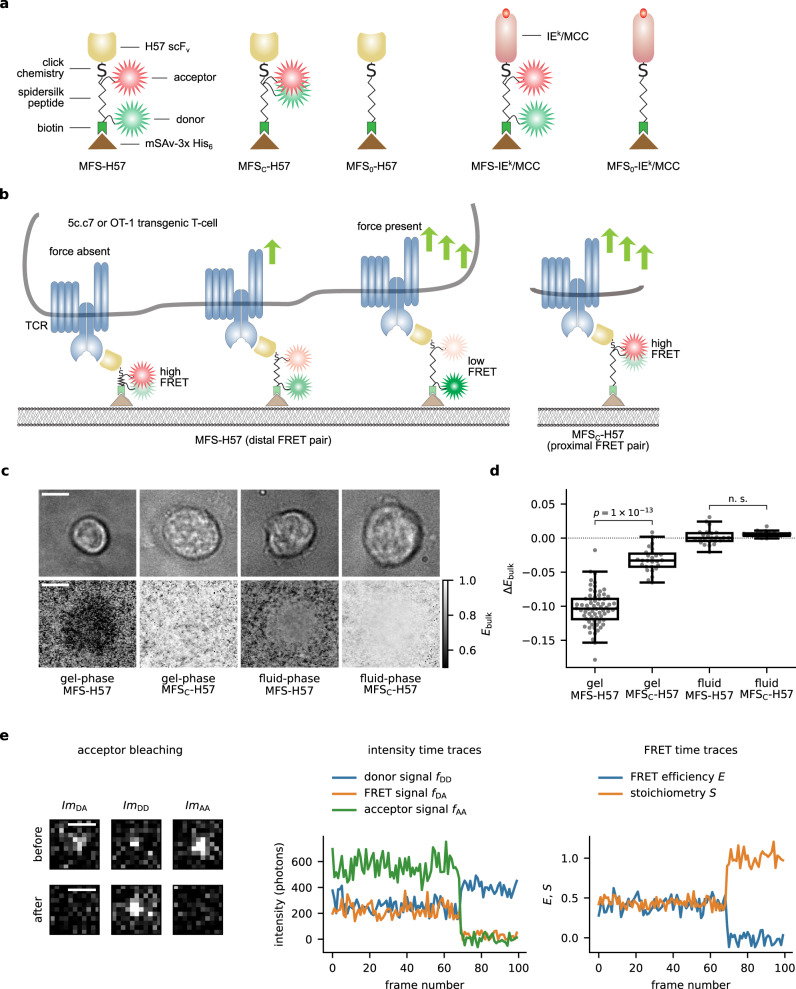
Fig. 1
FRET-based sensor designed to detect forces on a single-molecule level .
a Schematic illustration of the force sensor constructs MFS-H57, and MFS-IE k /MCC, the control construct MFS C -H57, and the unlabeled constructs MFS 0 -H57 and MFS 0 -IE k /MCC. b Exertion of forces...
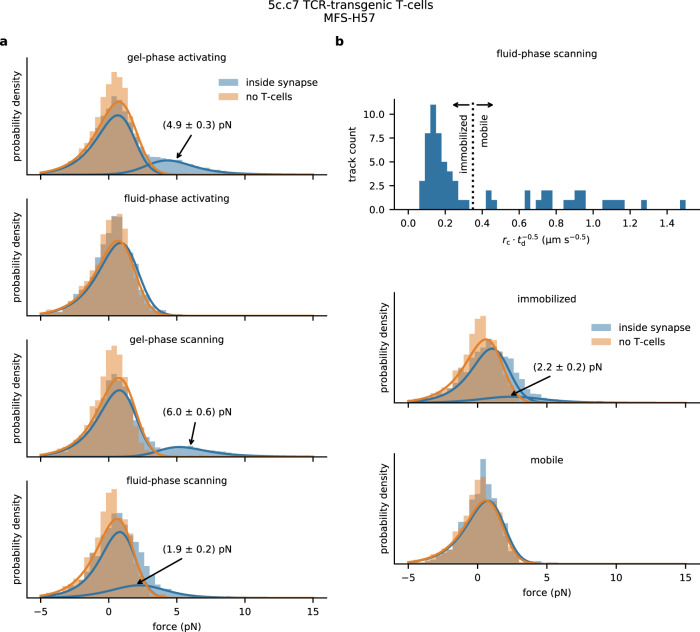
Fig. 2
Single-molecule pulling forces exerted via individual TCRs on the H57-functionalized molecular force sensor .
a Single-molecule TCR-imposed forces determined within synapses of activated or scanning T-cells confronted with gel-phase (DPPC) or fluid-phase (POPC) SLBs. Experiments were performed on 5c.c7 T-cell...
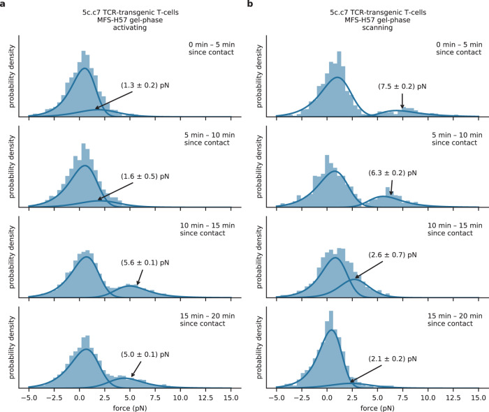
Fig. 3
Single-molecule force profiles in the course of synapse formation .
We used MFS-H57 data recorded on 5c.c7 T-cells contacting activating ( a ) or non-activating ( b ) gel-phase SLBs. Data were grouped with respect to the time elapsed since the corresponding T-cell fir...
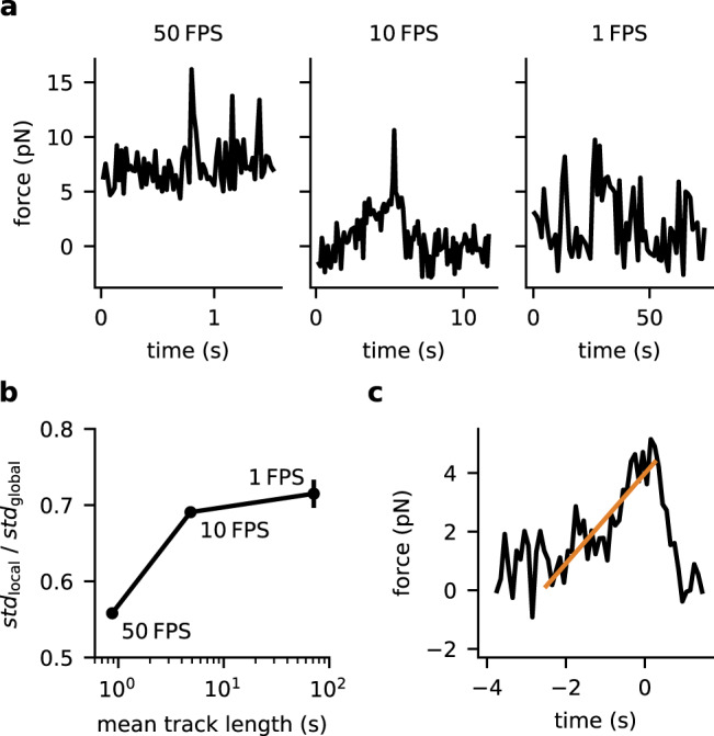
Fig. 4
Temporal analysis of TCR-applied forces observed for activated T-cells confronted with gel-phase SLBs .
a Representative single-molecule force traces recorded at indicated frame rates. We observed transitions within force trajectories only in traces recorded at low frame rates, whereas trajectories reco...
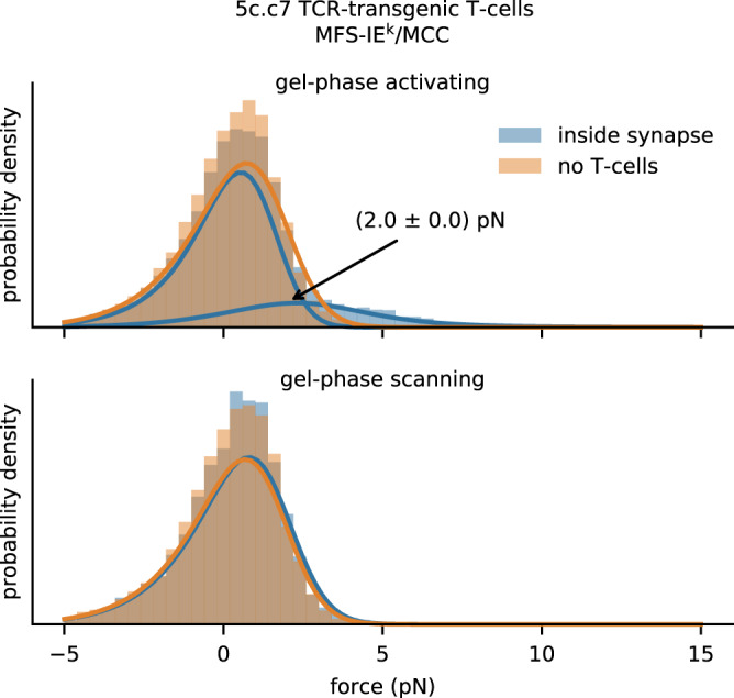
Fig. 5
Single-molecule pulling forces exerted via single TCRs on the pMHC-functionalized molecular force sensor .
Single-molecule analysis of MFSu2013IE k /MCC on gel-phase SLBs recorded under activating (top) or scanning conditions (bottom), using antigen-experienced 5c.c7 TCR-transgenic T-cells. We observed a s...
Figure images are served from the NIH/NLM PubMed Central Open Access Subset or Europe PMC; copyright remains with the publishers and authors.
💬 Discussion
0 commentsNo comments yet. Be the first to start a discussion!
Leave a Comment