Abstract
Single-molecule localization microscopy is a powerful tool for visualizing subcellular structures, interactions and protein functions in biological research. However, inhomogeneous refractive indices inside cells and tissues distort the fluorescent signal emitted from single-molecule probes, which rapidly degrades resolution with increasing depth. We propose a method that enables the construction of an in situ 3D response of single emitters directly from single-molecule blinking datasets, and therefore allows their locations to be pinpointed with precision that achieves the Cramér-Rao lower bound and uncompromised fidelity. We demonstrate this method, named in situ PSF retrieval (INSPR), across a range of cellular and tissue architectures, from mitochondrial networks and nuclear pores in mammalian cells to amyloid-β plaques and dendrites in brain tissues and elastic fibers in developing cartilage of mice. This advancement expands the routine applicability of super-resolution microscopy from selected cellular targets near coverslips to intra- and extracellular targets deep inside tissues.
🔬 Techniques
✨ Fluorophores
🧪 Sample Preparation
🔬 Cell Lines
🏭 Microscope Brands
🧪 Reagent Suppliers
📷 Detectors
🎨 Filters
💻 Software Details
💻 Code & Software
💾 Data Repositories
🏛️ Research Organizations (ROR)
Affiliated research institutions:
📋 Methods
Experimental demonstration of INSPR in whole cells
We first imaged immunofluorescence-labeled TOM20 in COS-7 cells in the biplane setup ( Fig. 3f – s , Extended Data Fig. 6 , Supplementary Video 4 ). To investigate the feasibility of INSPR when imaging above the coverslip surface, we created a 9-μm-thick sample cavity filled with water-based imaging medium between two coverslips, with the cells on the upper one. By using INSPR, the interconnected mitochondrial network was clearly resolved, where the x-z and y-z cross sections revealed the membrane contour of mitochondria in the axial direction ( Fig. 3f – h ). Examining reconstructions of the same field of view from both INSPR and the in vitro phase retrieval method based on fluorescent beads attached on the coverslip 19 , 28 , we found INSPR resolved the surface contour of each organelle with high resolution in 3D ( Supplementary Video 4 ), whereas reconstructions using the in vitro approach exhibited both distortion and decreased resolution ( Fig. 3i – p , Extended Data Fig. 6b ). Intensity profiles of 25 typical outer membrane contours (positions shown in Extended Data Fig. 6a ) also demonstrated a consistent improvement in resolution ( Fig. 3q , Extended Data Fig. 6e ). To further explain this difference, we compared the INSPR retrieved PSF models with the in vitro one ( Fig. 3r , s , Extended Data Fig. 6c , d ). The amount of sample-induced aberrations such as spherical and coma from optical sections increased together with the imaging depth, which was reflected by the INSPR retrieved pupils, their decomposed Zernike amplitudes, and their axially stretched PSFs. In contrast, the PSF retrieved from fluorescent beads characterized instrument imperfections but failed to take into account sample-induced aberrations and their depth-dependent variations due to its in vitro nature. Furthermore, we compared INSPR with other state-of-the-art in vitro localization methods such as ZOLD-3D 24 , cubic spline 21 , and microsphere-calibrated Gaussian fitting 23 by reconstructing immunofluorescence-labeled TOM20 in COS-7 cells in the astigmatism-based setup ( Extended Data Figs. 4 , 5 , Supplementary Notes 1.3 , 1.4 , 3.5 ). While sample-induced aberrations vary from specimen to specimen deteriorating the axial reconstruction for in vitro algorithms, our results show that INSPR is able to consistently achieve high-resolution 3D reconstructions as shown in the 200-nm-thick axial cross section images ( Extended Data Figs. 4b – g , 5b – e , h – k ). We next tested INSPR by reconstructing immunofluorescence-labeled nucleoporin Nup98 in COS-7 cells ( Fig. 4 , Extended Data Fig. 7 , Supplementary Video 5 ), which localizes near the center channel of the nuclear pore complex (NPC). We first reconstructed a super-resolution 3D volume of Nup98 within a relatively small depth of 3.3 μm and found individual ring-like structures covered the bottom surface of the nuclear envelope, displaying slight invaginations and undulations ( Fig. 4a – d ). We then reconstructed Nup98 on the entire nuclear envelope with a total thickness of 6.4 μm ( Fig. 4e – l ), and found that not only the individual pores were distinctly resolved throughout the entire envelope, but also the ultra-structures were resolved at both bottom and top surfaces of the nucleus ( Fig. 4f , g , Supplementary Video 5 ). The diameters of these resolved Nup98 structures were 60±9 nm and 57±11 nm ( Extended Data Fig. 7e , 40 measurements for each sample, profile positions shown in Extended Data Fig. 7a , c ), which was consistent with being localized to the NPC channel walls and its labeling using IgG antibody molecules. Lateral profiles of single boundaries ( i.e . ring thickness) of the observed structures resulted in σ y of 14±3 nm and 11±3 nm ( Extended Data Fig. 7f , 80 measurements for each sample, profile positions shown in Extended Data Fig. 7a , c ), while σ z of the top envelope surface (46±12 nm) was similar to that of the bottom surface (48±9 nm and 36±11 nm) ( Extended Data Fig. 7g , 20 measurements for the bottom surface of the 3.3-μm-thick volume and 10 measurements for each surface of the 6.4-μm-thick volume, profile positions shown in Extended Data Fig. 7b , d ). We notice that when using the in vitro approach, the thickness of the central cross section from the entire nuclear envelope was shrunk 32% compared to INSPR ( Extended Data Fig. 7h , i ) due to the inaccurate PSF model.
Show full methods section
Experimental demonstration of INSPR in whole cells
We first imaged immunofluorescence-labeled TOM20 in COS-7 cells in the biplane setup ( Fig. 3f – s , Extended Data Fig. 6 , Supplementary Video 4 ). To investigate the feasibility of INSPR when imaging above the coverslip surface, we created a 9-μm-thick sample cavity filled with water-based imaging medium between two coverslips, with the cells on the upper one. By using INSPR, the interconnected mitochondrial network was clearly resolved, where the x-z and y-z cross sections revealed the membrane contour of mitochondria in the axial direction ( Fig. 3f – h ). Examining reconstructions of the same field of view from both INSPR and the in vitro phase retrieval method based on fluorescent beads attached on the coverslip 19 , 28 , we found INSPR resolved the surface contour of each organelle with high resolution in 3D ( Supplementary Video 4 ), whereas reconstructions using the in vitro approach exhibited both distortion and decreased resolution ( Fig. 3i – p , Extended Data Fig. 6b ). Intensity profiles of 25 typical outer membrane contours (positions shown in Extended Data Fig. 6a ) also demonstrated a consistent improvement in resolution ( Fig. 3q , Extended Data Fig. 6e ). To further explain this difference, we compared the INSPR retrieved PSF models with the in vitro one ( Fig. 3r , s , Extended Data Fig. 6c , d ). The amount of sample-induced aberrations such as spherical and coma from optical sections increased together with the imaging depth, which was reflected by the INSPR retrieved pupils, their decomposed Zernike amplitudes, and their axially stretched PSFs. In contrast, the PSF retrieved from fluorescent beads characterized instrument imperfections but failed to take into account sample-induced aberrations and their depth-dependent variations due to its in vitro nature. Furthermore, we compared INSPR with other state-of-the-art in vitro localization methods such as ZOLD-3D 24 , cubic spline 21 , and microsphere-calibrated Gaussian fitting 23 by reconstructing immunofluorescence-labeled TOM20 in COS-7 cells in the astigmatism-based setup ( Extended Data Figs. 4 , 5 , Supplementary Notes 1.3 , 1.4 , 3.5 ). While sample-induced aberrations vary from specimen to specimen deteriorating the axial reconstruction for in vitro algorithms, our results show that INSPR is able to consistently achieve high-resolution 3D reconstructions as shown in the 200-nm-thick axial cross section images ( Extended Data Figs. 4b – g , 5b – e , h – k ). We next tested INSPR by reconstructing immunofluorescence-labeled nucleoporin Nup98 in COS-7 cells ( Fig. 4 , Extended Data Fig. 7 , Supplementary Video 5 ), which localizes near the center channel of the nuclear pore complex (NPC). We first reconstructed a super-resolution 3D volume of Nup98 within a relatively small depth of 3.3 μm and found individual ring-like structures covered the bottom surface of the nuclear envelope, displaying slight invaginations and undulations ( Fig. 4a – d ). We then reconstructed Nup98 on the entire nuclear envelope with a total thickness of 6.4 μm ( Fig. 4e – l ), and found that not only the individual pores were distinctly resolved throughout the entire envelope, but also the ultra-structures were resolved at both bottom and top surfaces of the nucleus ( Fig. 4f , g , Supplementary Video 5 ). The diameters of these resolved Nup98 structures were 60±9 nm and 57±11 nm ( Extended Data Fig. 7e , 40 measurements for each sample, profile positions shown in Extended Data Fig. 7a , c ), which was consistent with being localized to the NPC channel walls and its labeling using IgG antibody molecules. Lateral profiles of single boundaries ( i.e . ring thickness) of the observed structures resulted in σ y of 14±3 nm and 11±3 nm ( Extended Data Fig. 7f , 80 measurements for each sample, profile positions shown in Extended Data Fig. 7a , c ), while σ z of the top envelope surface (46±12 nm) was similar to that of the bottom surface (48±9 nm and 36±11 nm) ( Extended Data Fig. 7g , 20 measurements for the bottom surface of the 3.3-μm-thick volume and 10 measurements for each surface of the 6.4-μm-thick volume, profile positions shown in Extended Data Fig. 7b , d ). We notice that when using the in vitro approach, the thickness of the central cross section from the entire nuclear envelope was shrunk 32% compared to INSPR ( Extended Data Fig. 7h , i ) due to the inaccurate PSF model.
Online Methods
Preparation of fluorescent beads on coverslips 25-mm-diameter coverslips (CSHP-No1.5–25, Bioscience Tools) were cleaned successively in ethanol (2701, Decon) and HPLC grade water (W5–4, Fisher Chemical) three times, and then dried with compressed air. 100-nm-diameter crimson beads (custom-designed, Invitrogen) were diluted to 1:100,000 in deionized water. 200 μL of poly-L-lysine solution (P4707, Sigma-Aldrich) was added on the coverslip, incubated for 20 min and subsequently rinsed with deionized water. 200 μL of diluted bead solution was added on the center of the coverslip and was incubated for 20 min at room temperature (RT). The coverslip was subsequently rinsed with deionized water and drained. The coverslip was placed on a custom-made holder, and 20 μL of 38% 2,2’-Thiodiethanol (166782, Sigma-Aldrich) in 1×PBS (10010023, Gibco) was added on its center. Another 25-mm-diameter coverslip (also cleaned by using the above protocol) was placed on top of this coverslip. This coverslip sandwich was sealed with two-component silicone dental glue (Twinsil speed 22, Dental-Produktions und Vertriebs GmbH).
Preparation of fluorescent beads embedded in agarose gel
A solution containing 1 mL of 1×PBS and 20 mg of agarose powder (A9045, Sigma-Aldrich) was added into a cube, vortexed, and then heated until 70 ℃. 2,2’-Thiodiethanol was added into the solution to adjust the refractive index until it increased to 1.352 to match the refractive index of the imaging medium. 100-nm-diameter crimson beads were diluted to 1:100,000 in this agarose gel solution. A 25-mm-diameter coverslip was placed on a custom-made holder, and 100 μL of the diluted bead solution was added on its center. Another cleaned coverslip was placed on top of this coverslip. This coverslip sandwich was put into the fridge until the agarose gel was solidified. Then this coverslip sandwich was sealed with two-component silicone dental glue. Preparation of Alexa Fluor 647 labeled microspheres on coverslips A solution containing 500 μL of deionized water, 500 μL of 1×PBS, 50 μL of 9.78 μm diameter biotin-coated microsphere solution (CP10000, Bangslab), and 0.5 μL of streptavidin-functionalized Alexa Fluor 647 ( S21374 , Invitrogen) was prepared. This solution was centrifuged for 20 min at 1340 rpm. The liquid was removed and replaced with 500 μL of 1×PBS. 100 μL of the vortexed solution was added on the center of a 25-mm-diameter coverslip, incubated for 20 min at RT, and sequentially rinsed with deionized water. This coverslip was placed on a custom-made holder, and 20 μL of imaging buffer (10% (w/v) glucose in 50 mM Tris (JT4109, J.T.Baker), 50 mM NaCl (S271-500, Fisher Chemical), 10 mM MEA (M6500, Sigma-Aldrich), 50 mM BME (M3148, Sigma-Aldrich), 2 mM COT (138924, Sigma-Aldrich), 2.5 mM PCA (37580, Sigma-Aldrich), and 50 nM PCD (P8279, Sigma-Aldrich), pH 8.0) was added on top of the coverslip. Then another cleaned coverslip was placed on top of the imaging buffer. This coverslip sandwich was sealed with two-component silicone dental glue.
Cell culture
COS-7 cells (CRL-1651, ATCC) were immunofluorescence-labeled with TOM20, α-tubulin, and Nup98. COS-7 cells were grown on coverslips in 6-well plates and cultured in DMEM (30–2002, ATCC) with 10% FBS (30–2020, ATCC) and 1% Penicillin-Streptomycin (15140122, Gibco) at 37 °C with 5% CO 2 until their confluence reaches about 80%. BS-C-1 cells (CCL-26, ATCC) in collagen embedded 3D cultures were immunofluorescence-labeled with α-tubulin. 50,000 BS-C-1 cells were centrifuged and re-suspended in 100 μL of 4 mg/mL collagen I (5201–1KIT, Advanced BioMatrix). The suspension containing collagen I and BS-C-1 cells was then dispensed onto coverslips in 6-well plates. After incubation at 37 °C for 20 min to solidify the collagen, cells on the coverslips were cultured in EMEM (30–2003, ATCC) with 10% FBS at 37 °C with 5% CO 2 until their confluence reaches about 80%. Fixation and labeling of TOM20, α-tubulin, and Nup98 In preparation of TOM20 and α-tubulin specimens, cultured cells were first fixed with 37 °C pre-warmed 3% PFA (15710, Electron Microscopy Sciences) and 0.5% GA (16019, Electron Microscopy Sciences) in 1×PBS at RT for 15 min. In preparation of Nup98 specimens, cultured cells were first rinsed with 37 °C pre-warmed 2.4% PFA in 1×PBS for 20 s, and then extracted with 37 °C pre-warmed 0.4% Triton X-100 (X100, Sigma-Aldrich) in 1×PBS for 3 min. Then, cells were fixed with 2.4% PFA in 1×PBS for 30 min. After fixation, cells were washed twice with 1×PBS and then quenched with freshly-prepared 0.1% NaBH 4 (452882, Sigma-Aldrich) in 1×PBS for 7 min. Subsequently, cells were washed three times with 1×PBS and then treated with blocking buffer (3% BSA (001-000-162, Jackson ImmunoResearch) and 0.2% Triton X-100 in 1×PBS for TOM20 and α-tubulin, and 5% BSA in 1×PBS for Nup98) for 1 h, gently rocked at RT. Then, cells were incubated with primary antibodies (sc-11415, Santa Cruz Biotechnology, for TOM20; T5168, Sigma-Aldrich, for α-tubulin; and 2598, Cell Signaling Technology, for Nup98; all diluted at 1:500) at 4 °C overnight. After washed three times for 5 min each time with wash buffer (0.05% Triton X-100 in 1×PBS), cells were then incubated with secondary antibodies (A21245 and A21236, Invitrogen, for Alexa Fluor 647, diluted at 1:500; DNA-conjugated anti-mouse P1, anti-rabbit P1, and anti-rabbit P4 32 for DNA-PAINT, diluted at 1:50) at RT for 5 h. Both primary and secondary antibodies were diluted in antibody dilution buffer (1% BSA and 0.2% Triton X-100 in 1×PBS for TOM20 and α-tubulin, and 5% BSA in 1×PBS for Nup98). After washed three times (5 min each time with wash buffer), cells were post-fixed with 4% PFA in 1×PBS for 10 min. Cells were then washed three times with 1×PBS and stored in 1×PBS at 4 °C until imaging. Fixation and labeling of amyloid β in mouse brain sections An 8-month-old 5XFAD mouse was anesthetized with Tribromoethanol (Avertin) 125–250mg/kg IP and transcardially perfused with saline. Brain was post-fixed with 4% PFA in PBST (0.1% Tween (0777, VWR) in 1×PBS) for 24 h. Tissue was then transferred to 30% sucrose (57-50-1, Fisher Chemical). Tissue was embedded in O.C.T. compound (23-730-571, Fisher Healthcare) and hemibrain was sagitally sectioned on a cryostat (CM1950, Leica) at 30 μm thick. Sections were stored at −20 °C in cryoprotectant (30% glycerol (G5516, Sigma-Aldrich) and 30% ethylene glycol (293237, Sigma-Aldrich) in 1×PBS). Prior to staining, sections were washed three times in PBST for 10 min each time and then treated for antigen retrieval with 10 mM sodium citrate (S279–500, Fisher Chemical) and 0.5% Tween in PBST at 85 °C for 10 min. Sections were blocked in normal donkey serum (D9663, Sigma-Aldrich) for 1 h and incubated with anti-β-amyloid antibody (2454, Cell Signaling Technology) at 4 °C overnight. Following three PBST washes, sections were then stained with donkey anti-rabbit Alexa Fluor 647 conjugated antibody ( A31573 , Invitrogen) at RT for 1 h. Both primary and secondary antibodies were diluted to 1:1000 in blocking buffer. Nuclei were stained with DAPI (10236276001, Sigma-Aldrich) diluted to 1:10,000 in PBST at RT for 2 min. Sections were then wet mounted onto coverslips and dried at 4 °C overnight before imaging. Fixation and labeling of ChR2-EYFP in mouse brain sections To perform infections, Ai32 mice (male postnatal day 89 and 273, RCL-ChR2(H134R)/EYFP, Jackson Lab) were first anesthetized with inhaled isoflurane (5% for induction, and 1.5% for maintenance in room air, using SomnoSuite system). Then the primary visual cortex was identified (stereotaxic coordinates: 0.3 mm anterior, 3.0 mm lateral, relative to the lambda reference point) and a small craniotomy was made using a dental drill to allow injection glass pipette to go in. 200 nL of pAAV-Ef1a-mCherry-IRES-Cre (55632-AAVrg, Addgene) was injected at 300 μm and 700 μm underneath the brain surface (1 nL/s, 100 nL for each depth) using a micro-injector (3000037, Drummond Scientific). After injection, metabond dental cement (Parkell) was applied on top of the mouse skull to form a protective head cap. 5 weeks were allowed for viral infection and protein expression before perfusion. To perform trans-cardiac perfusion, mice were first anesthetized with 100 mg/kg ketamine (59399-114-10, Akron) and 16 mg/kg xylazine (343750, HVS) through intra-peritoneal injection. After anesthetized state was confirmed by toe pinch, the abdomen was opened to expose the heart. A needle was inserted into the left ventricle and a small incision was made on the right atrium of the heart. Mice were first perfused with 1×PBS (1:10 diluted from DSP32060, Dot Scientific) until the liver was cleared, and then with 4% PFA (P6148, Sigma-Aldrich) in 1×PBS for fixation. Mouse brains were carefully extracted and post-fixed in 4% PFA for 12–24 h before slicing. Brain tissues were sliced using a vibrating microtome (1000 Plus, TPI Vibratome) at 50 μm thick. Before immunohistochemistry, slices were washed three times for 15 min each time in wash buffer (0.1% Triton X-100 in 1×PBS), then treated with blocking buffer (5% BSA (A9647, Sigma-Aldrich) in 1×PBS) at RT for 1.5 h. After that, slices were incubated with chicken anti-GFP antibody (ab13970, Abcam, diluted to 1:1000 in blocking buffer) at 4°C overnight, washed three times (15 min each time with wash buffer), and then incubated with goat anti-chicken Alexa Fluor 647 conjugated antibody (A21449, Invitrogen, diluted to 1:600 in wash buffer) at RT for 2 h. Slices were then wet mounted onto coverslips and dried at 4 °C overnight before imaging. Fixation and labeling of elastic fibers in developing cartilage E14.5 mouse embryos were generated by the timed mating of wild type C57Bl/6 mice. Mice were euthanized via CO 2 inhalation and confirmed by cervical dislocation. Embryos were removed from the uterine horns and rinsed with 1×PBS. Forelimbs were removed from the embryos and mounted in 1% low gelling agarose cubes. Agarose cubes were submerged in 0.05% SDS (0837, VWR) and 2% Penicillin-Streptomycin in 1×PBS, and gently rocked at RT. The SDS buffer was replaced every 48 h until decellularization was completed (3–5 d). Upon decellularization, agarose cubes were rinsed with 1×PBS for 1 h, and then fixed with 4% PFA (J19943K2, Thermo Scientific) in 1×PBS for 1 h, rinsed with 1×PBS for 1 h again gently rocked at RT. Forelimbs were removed from the agarose cubes for cryosectioning. Forelimbs were submerged in 15% sucrose (84097, Sigma-Aldrich) at 4 °C until equilibrated (indicated by the specimen sinking to the bottom of the tube), and then submerged in 30% sucrose at 4 °C until equilibrated. Forelimbs were embedded in O.C.T. compound (4583, Sakura Finetek), frozen in dry-ice-cooled isopentane, and stored at −80 °C until sectioning. 20-μm-thick cryosections containing cartilage from the humerus were collected on coverslips and stored at −20 °C. Before staining, cryosections were rinsed with 1×PBS for 5 min to remove any residual O.C.T. compound, fixed with 4% PFA in 1×PBS for 15 min, and rinsed with 1×PBS for 5 min again. Cryosections were then quenched with 0.1% NaBH 4 in 1×PBS for 15 min, and washed with 1×PBS for 5 min. Cryosections were blocked with 10% donkey serum (S30, Sigma-Aldrich) and 0.2% BSA (A9418, Sigma-Aldrich) in 1×PBS for 1 h, and then incubated with Alexa Fluor 647 conjugated WGA ( W32466 , Invitrogen) diluted to 1:200 in 1×PBS at 4 °C overnight. After that, cryosections were washed three times with 1×PBS and stored in 1×PBS at 4 °C until imaging.
Imaging buffers and sample mounting
Immediately before imaging samples labeled with Alexa Fluor 647, the coverslip with specimens on top of it was placed on a custom-made holder. 20–40 μL of imaging buffer (10% (w/v) glucose in 50 mM Tris, 50 mM NaCl, 10 mM MEA, 50 mM BME, 2 mM COT, 2.5 mM PCA, and 50 nM PCD, pH 8.0) was added on top of the coverslip. Then another cleaned coverslip was placed on top of the imaging buffer. This coverslip sandwich was sealed with melted valap (1:1:1 [w/w/w] mixture of lanolin, paraffin, and Vaseline (L7387, 18634, and 16415, Sigma-Aldrich)) or two-component silicone dental glue. The sample cavity with immunofluorescence-labeled cells on the top coverslip was prepared in a similar way by placing the cleaned coverslip at the bottom and the coverslip with cells on top of it with the cell side surface facing down. Immediately before imaging samples tagged with DNA-PAINT probes, the coverslip with cells on top of it was placed on a cell chamber (A7816, Invitrogen). 600 μL of imaging buffer (2 nM ATTO 655 conjugated DNA imager strand diluted in 500 mM NaCl in 1×PBS) was added into the chamber. In the distorted wavefront control experiment, P1 imager strand was used to image mitochondria. In Exchange-PAINT imaging, the chamber was mounted firmly on the sample stage to minimize the lateral drift. We first added imaging buffer with P4 strand to image mitochondria, and then used syringes to remove the buffer, wash samples with 1×PBS for several times, and add imaging buffer with P1 strand to image microtubules.
Microscope Setup
The system ( Extended Data Fig. 1f ) was built around an Olympus IX-73 microscope stand (IX-73, Olympus America) equipped with a 100×/1.35-NA silicone-oil-immersion objective lens (FV-U2B714, Olympus America) and a PIFOC objective positioner (ND72Z2LAQ, Physik Instrumente). Three laser lines at wavelengths of 642 nm (2RU-VFL-P-2000–642-B1R, MPB Communications), 560 nm (2RU-VFL-P-500–560, MPB Communications), and 405 nm (DL-405–100, Crystalaser) were coupled into a polarization-maintaining single-mode fiber (PM-S405-XP, Thorlabs) after passing through an acousto-optic tunable filter (AOTFnC-400.650-TN, AA Opto-electronic) for wavelength selection and power modulation. The excitation light coming out of the fiber was focused to the pupil plane of the objective lens after passing through a filter cube holding a quadband dichroic mirror (Di03-R405/488/561/635-t1, Semrock). The focus of excitation light in the pupil plane could be translated sideways by a mirror conjugated to the sample plane for switching between epi-illumination and highly inclined and laminated optical sheet (HILO) imaging modalities 46 . Additionally, a transmitted Köhler illuminator inside the microscope stand equipped with a motorized shutter (87–208, Edmund Optics) illuminated the sample between acquisition cycles for focus stabilization 47 . Besides, to observe the nucleus labeled with DAPI, an alternative illumination module was used, where light from a mercury light source (U-LH100HG, Olympus America) was directed by a motorized flip mirror, passed through a filter cube holding a bandpass filter (AT350/50x, Chroma) and a dichroic mirror (T400LP, Chroma), and then illuminated the sample. The pupil plane of the objective lens was imaged onto a deformable mirror (Multi-3.5, Boston Micromachines), which allowed for introducing controlled amount of wavefront aberrations to test the performance of INSPR experimentally. The fluorescent signal was magnified by relay lenses arranged in a 4 f alignment to a final magnification of ~54, and then was split with a 50/50 non-polarizing beam splitter (BS016, Thorlabs) mounted on a kinematic base (KB25/M, Thorlabs). The separated fluorescent signals were delivered by two mirrors onto a 90° specialty mirror (47–005, Edmund Optics), passed through a motorized filter wheel holding five alternative bandpass filters (FF01–731/137–25 and FF01–600/52–25, Semrock; ET665LP, ET700/75m, and ET460/50m, Chroma), and were then projected on an sCMOS camera (Orca-Flash4.0v3, Hamamatsu) with an effective pixel size of 120 nm. The detection planes that received the signals transmitted and reflected by the beam splitter were referred as plane 1 and plane 2, respectively ( Extended Data Fig. 1g ). To adjust the distance between the two detection planes, two piezo inertia actuators (PIAK10 and PIA13, Thorlabs) were equipped on the mirror that delivered the reflected signal onto the 90° specialty mirror. When the system worked as an astigmatism-based setup, the beam splitter was removed so that the camera only detected the transmitted signal, while the correction collar of the objective lens was adjusted to minimize spherical aberrations. In this case, we used the deformable mirror (DM) to induce vertical astigmatism with an amplitude of +1.5 (unit: λ/2π). The imaging system was controlled by a custom-written program in LabVIEW (National Instruments). Data acquisition The SMLM setup is extremely susceptible to sample drift in the axial direction for its long data acquisition time, typically from tens of minutes to hours. To compensate this drift, we implemented a focus stabilization module 47 . Before fluorescence imaging, we recorded a series of bright-field images of the sample along the axial direction (from −1 to +1 μm, with a step size of 100 nm) as reference images. During fluorescence imaging, we recorded a real-time bright-field image of the sample after each acquisition cycle (1000 or 2000 frames, depending on the sample stability), and compared the similarities between this real-time image and reference images by calculating their 2D correlation. The correlation values of the most similar reference image and its nine adjacent images, together with their z positions, were fitted with third degree polynomials. The z position corresponding to the maximum correlation value in the fitting curve was treated as the sample drift. Then we moved the objective lens in the inverse direction to compensate this drift. In this way, focus stabilization can be achieved during data acquisition. The biplane datasets for measuring the biplane distance ( Extended Data Fig. 1g ) and building the in vitro model ( Fig. 3f – s , Extended Data Figs. 6 – 10 ) were separately collected by imaging fluorescent beads on the coverslip or in the agarose gel over an axial range from −1.5 to +1.5 μm with a step size of 100 nm, and taking 50 frames per step with a frame rate of 10 Hz. The biplane distance ( Supplementary Note 2.1 ) was estimated to be 580 nm for distorted wavefront control ( Fig. 2e , f ), 286 nm for imaging TOM20 labeled with Alexa Fluor 647 ( Fig. 3f – s ), 568 nm for imaging dendrites with depths of 7 μm and 11 μm ( Extended Data Fig. 9 ), and 558 nm for all the other imaging sessions ( Figs. 4 – 6 ). The astigmatism-based dataset for building the in vitro cubic spline model ( Extended Data Fig. 4 ) was collected by imaging fluorescent beads on the coverslip over an axial range from −1 to +1 μm with a step size of 50 nm, and taking 50 frames per step with a frame rate of 10 Hz (~5 beads in each dataset, 3 datasets in total). Here we used DM to induce vertical astigmatism with an amplitude of +1.5 (unit: λ/2π). Due to instrument imperfections, the setup itself has vertical astigmatism with an amplitude of −0.3 (unit: λ/2π), so the resulting vertical astigmatism has an amplitude of +1.2 (unit: λ/2π) as prior knowledge. The astigmatism-based SMLM dataset for obtaining the calibration curve from microspheres ( Extended Data Fig. 5 ) was collected by imaging Alexa Fluor 647 labeled microspheres on the coverslip. The microsphere sample was first illuminated with the transmitted light to record a bright-field image at the equatorial plane of the microspheres, which was used to measure both the radius R and the center ( x 0 , y 0 ) of each microsphere. Then the objective lens was moved axially to the selected imaging depth. Before fluorescence imaging, bright-field images of this region were recorded over an axial range from −1 to +1 μm with a step size of 100 nm as reference images for focus stabilization. Then the blinking data were collected at the illumination of the 642-nm laser. The laser power was 17 kW/cm 2 to get low density of molecules. 1000 frames were collected per cycle with a frame rate of 50 Hz and ~15 cycles were collected. In biological imaging ( Figs. 2f , 3f – s , 4 – 6 , Extended Data Figs. 4 , 5 , 9 ), the sample was first excited with the 642-nm laser at a low intensity of ~50 W/cm 2 to find a region of interest. The depth from this region to the bottom coverslip was measured by recording a first position of the objective lens when the dusts on the bottom coverslip were in focus, then recording a second position of the objective lens when the region of interest was in focus. The difference between these two recorded positions was treated as the depth of this region. Before fluorescence imaging, bright-field images of this region were recorded over an axial range from −1 to +1 μm with a step size of 100 nm as reference images for focus stabilization. Then the blinking data were collected at a laser intensity of 2–6 kW/cm 2 and a frame rate of 50 Hz. For distorted wavefront control ( Fig. 2f ), 2000 frames were collected for each Zernike-based aberration mode with its amplitude set at ±1 (unit: λ/2π). For single-section imaging ( Extended Data Fig. 5 ), 2000 frames were collected per cycle and ~50 cycles were collected. For multi-section imaging ( Figs. 3f – s , 4 – 6 , Extended Data Figs. 4 , 9 ), the sample was scanned axially by translating the objective lens with a step size of 400 nm in biplane setup and 250 nm in astigmatism-based setup from the bottom to the top of the sample. 1000 or 2000 frames were collected for each cycle in one optical section, 5–14 optical sections were collected according to the thickness of the sample, and 8–25 cycles were collected in total ( Supplementary Table 1 ).
Animals
All animal procedures associated with mice were approved by Indiana University School of Medicine Institutional Animal Care and Use Committee (IACUC) and Purdue Animal Care and Use Committee (PACUC), and complied with all relevant ethical regulations. Reporting Summary Further information on research design is available in the Nature Research Reporting Summary linked to this article.
Data availability
The data that support the findings of this study are available from the corresponding authors upon request. Example data are available in software packages. 3D point clouds resolved by INSPR for Supplementary Videos 4 – 9 are provided from figshare ( https://doi.org/10.6084/m9.figshare.11962764 ). Code availability The INSPR toolbox for in situ model estimation and 3D localization is available as supplementary software . INSPR works for commonly used biplane and astigmatism configurations. Further updates will be made freely available at https://github.com/HuanglabPurdue/INSPR . The software package features an easy-to-use user interface including all steps of 3D single-molecule localization from INSPR model generation, pupil-based 3D localization (including both CPU and GPU versions), drift correction, volume alignment, to super-resolution image reconstruction.
Supplementary Material 1 2 3 1578395_Video1 1578395_Video2 1578395_Video3 1578395_Video4 1578395_Video5 1578395_Video6 1578395_Video7 1578395_Video8 1578395_Video9
📊 Figures
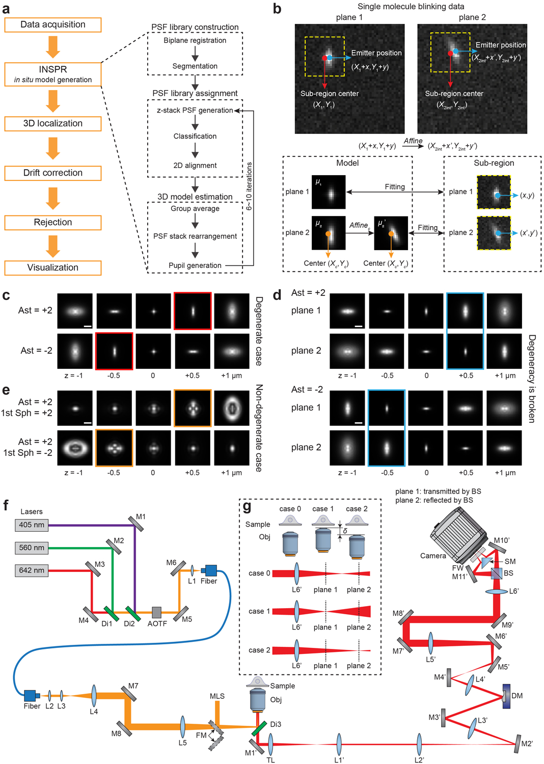
Extended Data Fig. 1.
INSPR framework, degeneracy illustration, and setup diagram.
(a) INSPR framework and detailed process of innsitu model generation. (b) Single molecules arenlocalized by a pair of channel-specific models which share the same shapeninformation with the correspond...
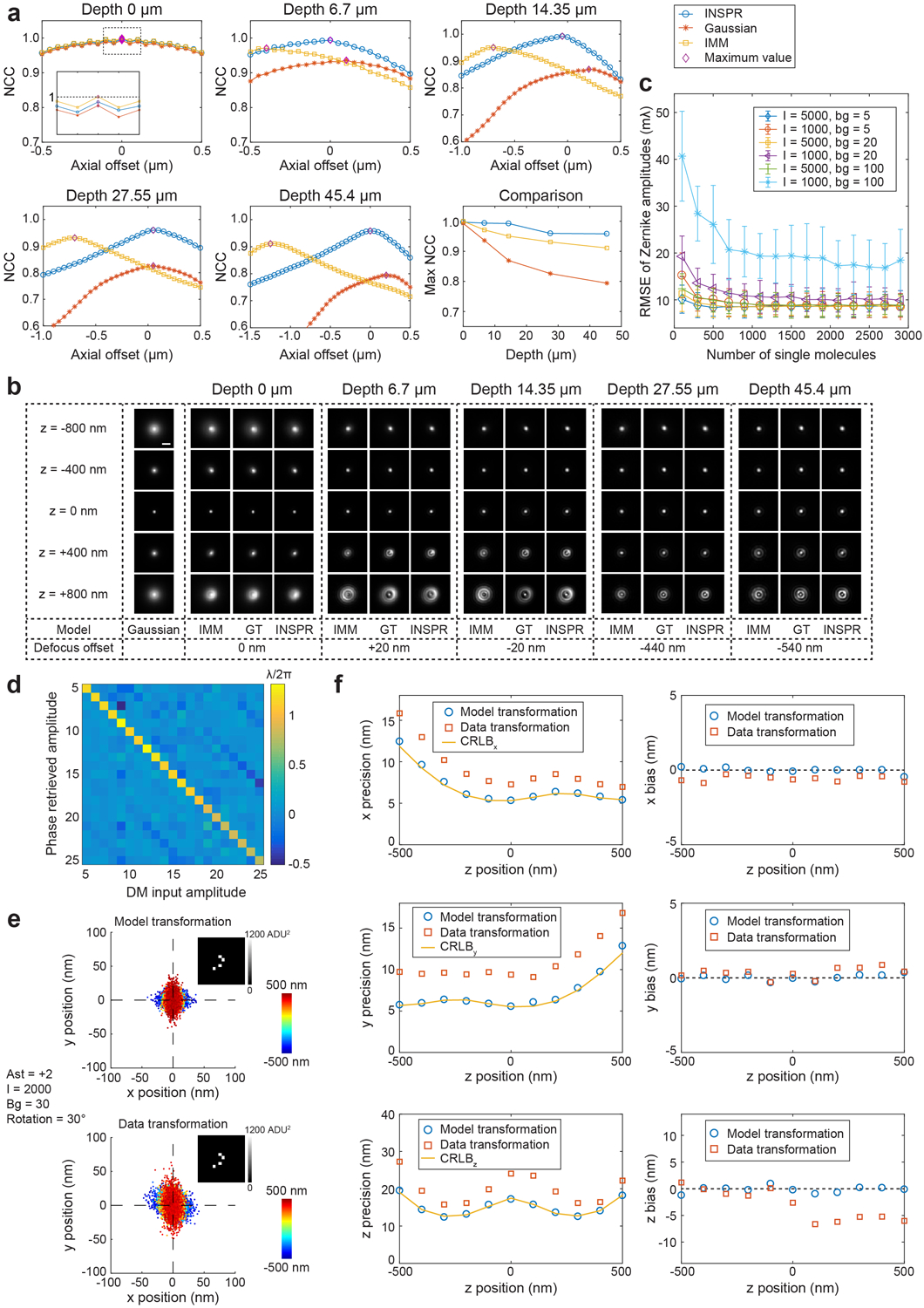
Extended Data Fig. 2.
Performance quantification of INSPR in biplane setup.
(a) Similarity between the ground truth 3D PSFs and then3D PSFs at different imaging depths when using INSPR (blue circles),nGaussian model (orange stars), and theoretical index mismatch model (IMM,ny...
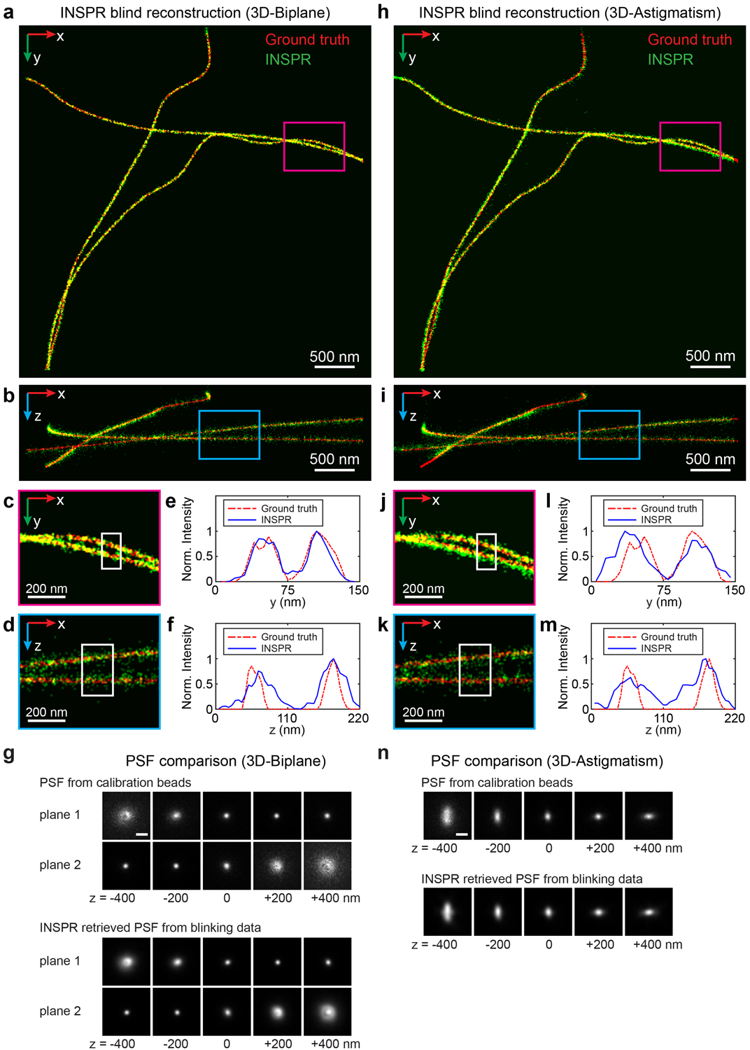
Extended Data Fig. 3.
Blind reconstruction of 3D training datasets of microtubules (MT0.N1.LD) from the SMLM challenge.
(a,b) x-y and x-z overviews of the microtubulesnresolved by INSPR from the 3D-Biplane data. (c,d) Enlarged x-ynand x-z views of the areas as indicated by the magenta and blue boxednregions in (a) and ...
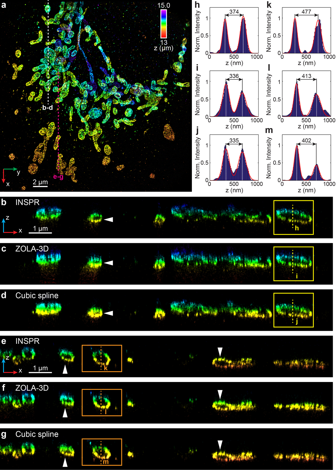
Extended Data Fig. 4.
3D super-resolution reconstructions of immunofluorescence-labeled TOM20 in COS-7 cells using INSPR, ZOLA-3D, and cubic spline in astigmatism-based setup.
(a) x-y overview of the mitochondrial network resolvednby INSPR, with a depth of 13 u03bcm from the coverslip. (bu2013d) x-z slices along the white dashed line in (a),nreconstructed using INSPR (b), Z...
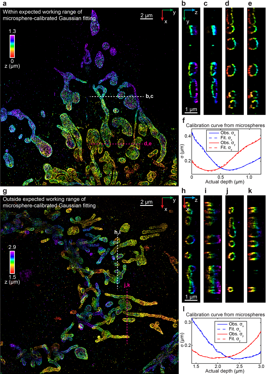
Extended Data Fig. 5.
3D super-resolution reconstructions of immunofluorescence-labeled TOM20 in COS-7 cells using INSPR and microsphere-calibrated Gaussian fitting in astigmatism-based setup.
(a) x-y overview of the mitochondrial network resolvednby INSPR on the bottom coverslip, within the expected working range ofnmicrosphere-calibrated Gaussian fitting. (bu2013e) y-znslices along the wh...
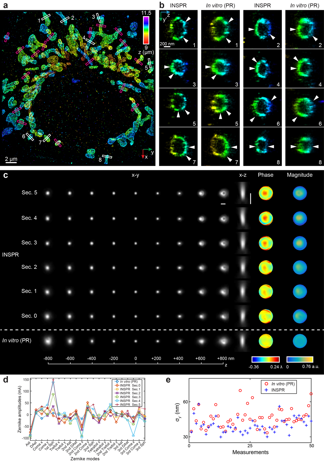
Extended Data Fig. 6.
3D super-resolution reconstructions of immunofluorescence-labeled TOM20 in COS-7 cells using INSPR and the in vitro method in biplane setup.
(a) x-y overview of the mitochondrial network showingnthe positions of 25 typical outer membrane contours as indicated by thenmagenta and white boxed regions. (b) Enlarged yu2019-z viewsnof the outer ...
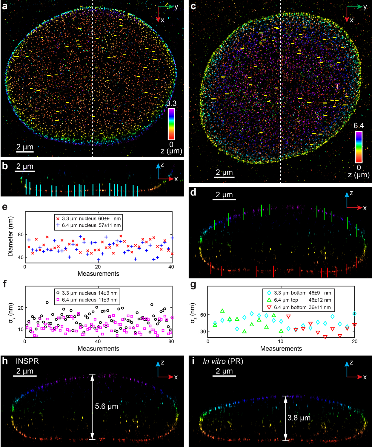
Extended Data Fig. 7.
3D super-resolution reconstructions of immunofluorescence-labeled Nup98 in COS-7 cells using INSPR and the in vitro method in biplane setup.
(a) x-y overview of the 3.3-u03bcm-thick volume ofnthe nucleus showing the positions of 40 typical Nup98 structures (yellownlines). (b) x-z slice along the white dashed line in (a),nshowing the positi...
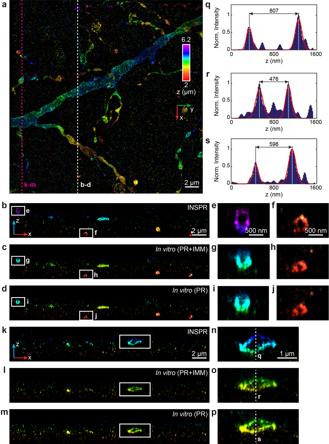
Extended Data Fig. 8.
3D super-resolution reconstructions of immunofluorescence-labeled ChR2-EYFP on dendrites using INSPR and in vitro methods in biplane setup (depth: 2 u2013 6.2 u03bcm).
(a) x-y overview of the super-resolution volume ofnimmunofluorescence-labeled ChR2-EYFP on dendrites resolved by INSPR, with andepth of 2 u03bcm from the coverslip. (bu2013d) x-znslices along the whit...
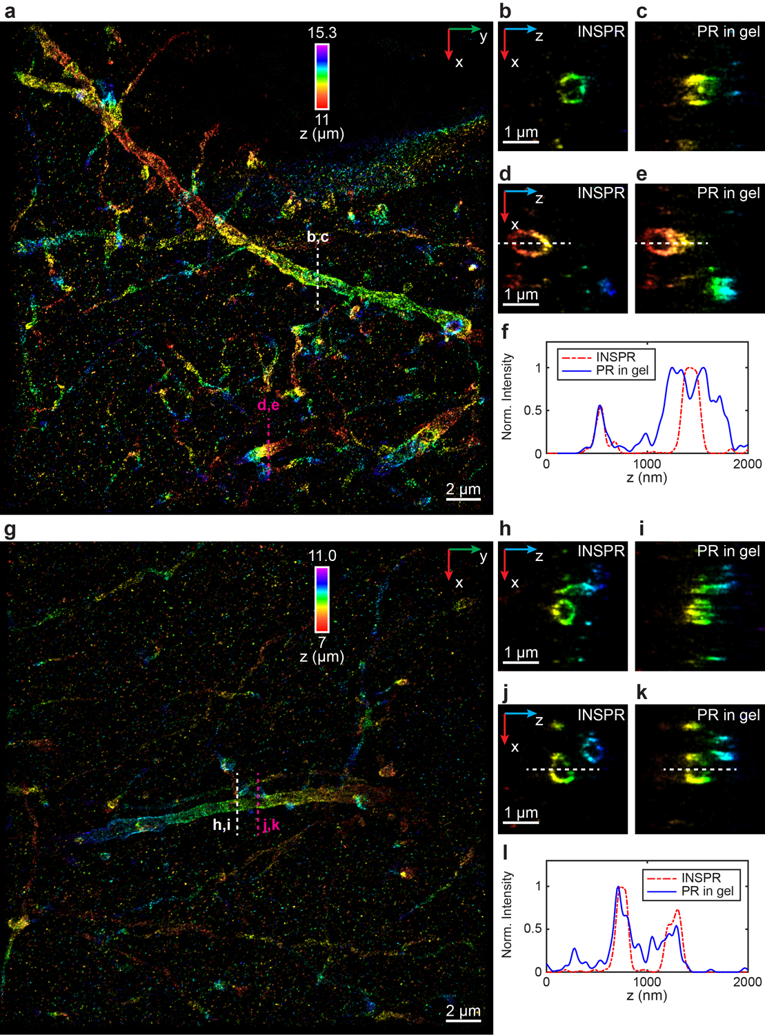
Extended Data Fig. 9.
3D super-resolution reconstructions of immunofluorescence-labeled ChR2-EYFP on dendrites using INSPR and phase retrieval method based on beads embedded in agarose gel in biplane setup.
(a) x-y overview of the super-resolution volume ofnimmunofluorescence-labeled ChR2-EYFP on dendrites resolved by INSPR, with andepth of 11 u03bcm from the coverslip. (bu2013e) x-znslices along the whi...
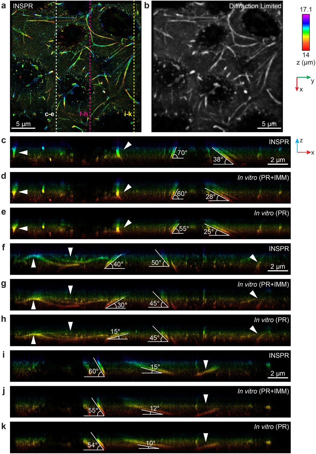
Extended Data Fig. 10.
3D super-resolution reconstructions of immunofluorescence-labeled elastic fibers in developing cartilage using INSPR and in vitro methods in biplane setup.
(a) x-y overview of the reconstructed volume ofnimmunofluorescence-labeled elastic fibers in developing cartilage usingnINSPR. (b) Diffraction-limited image of (a). (cu2013k) x-z slices along the whit...
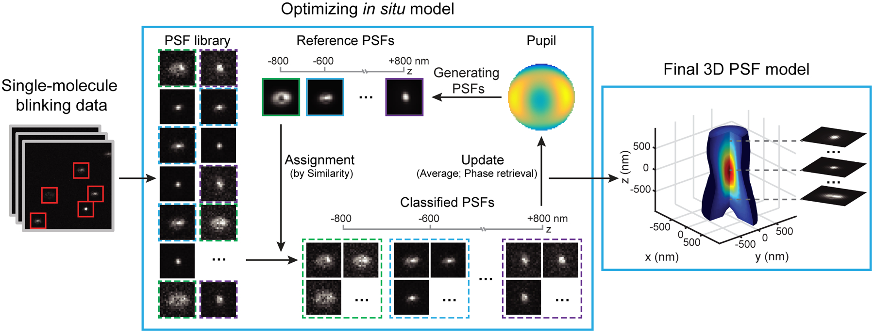
Fig. 1.
Concept of INSPR.
After the single-molecule dataset (left panel) is acquired, a PSFnlibrary is obtained. Starting with a constant pupil function, INSPR assigns eachndetected PSF to a temporary axial position according ...
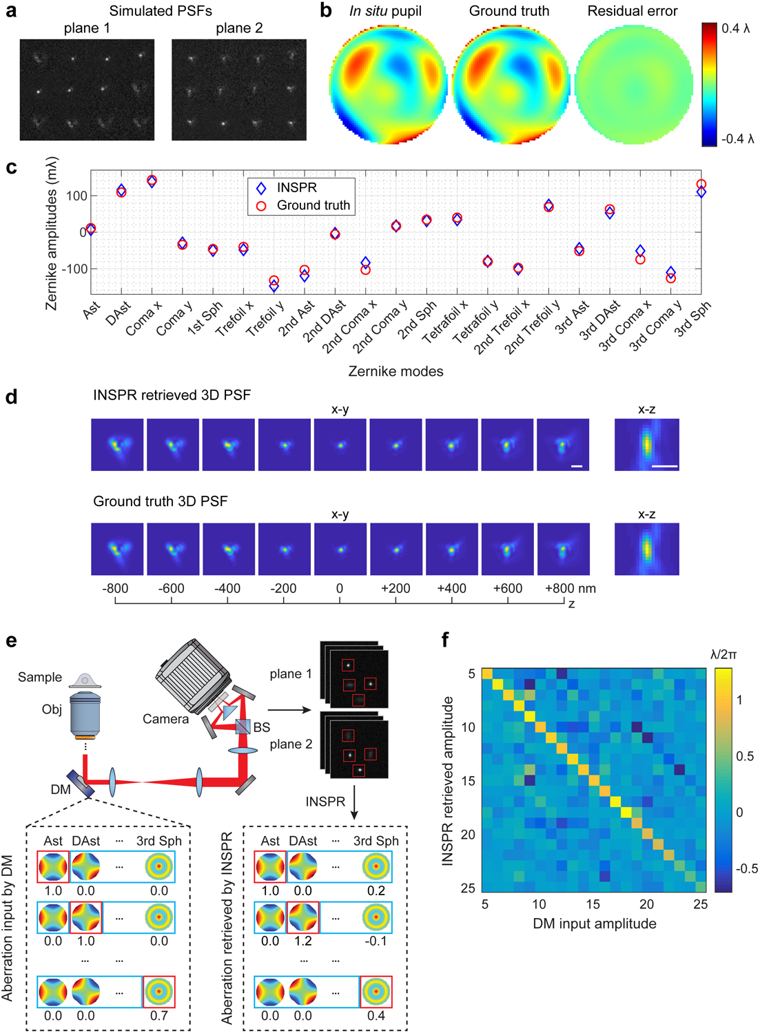
Fig. 2.
Performance quantification of INSPR.
(a) Simulated biplane single-molecule emission patternsnlocated randomly over an axial range from u2212800 to +800 nm with a knownnwavefront distortion. (b) Phase of the in situ pupil retrieved by INS...
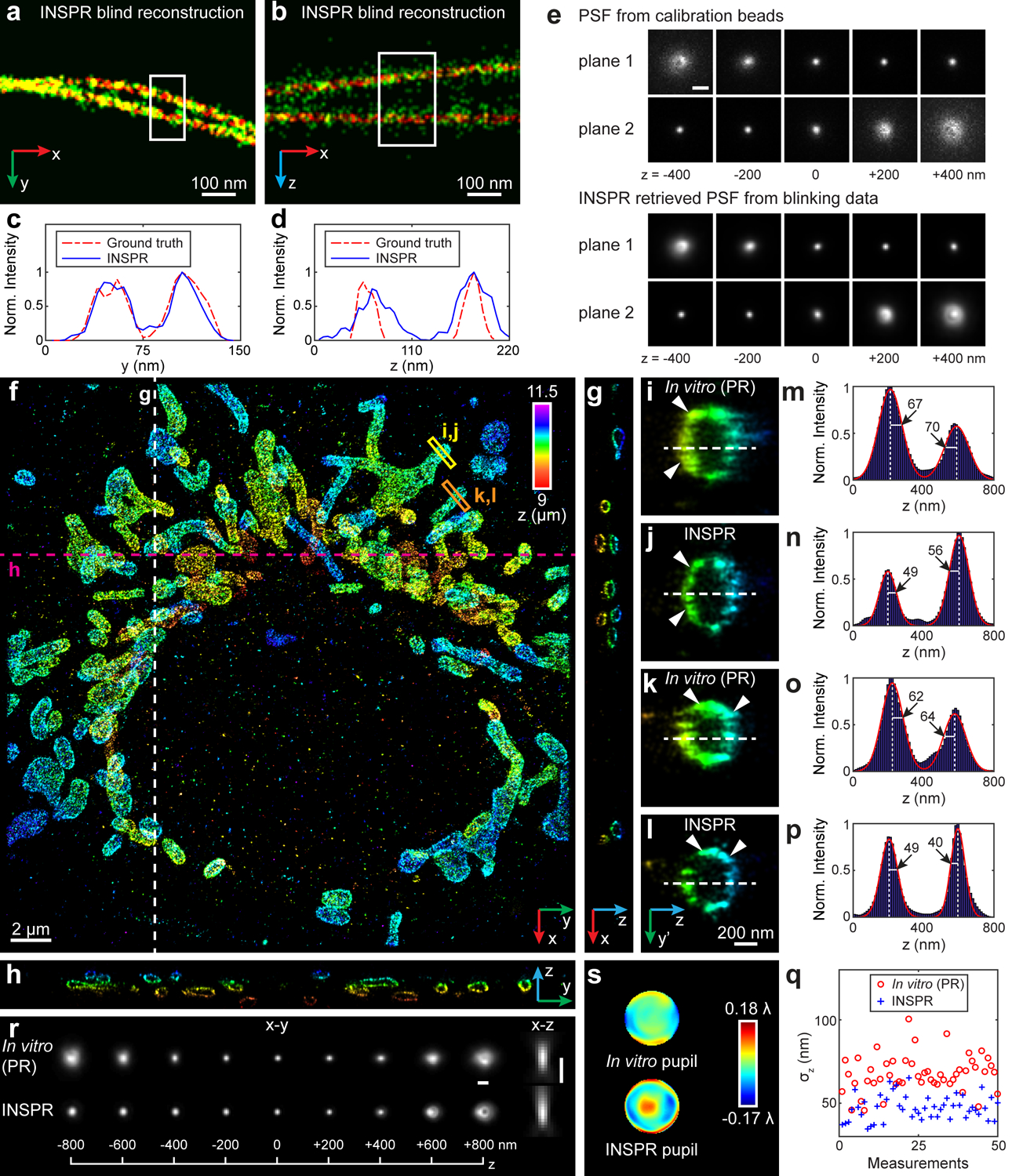
Fig. 3.
Blind reconstruction of microtubules from the SMLM challenge and 3D super-resolution reconstructions of immunofluorescence-labeled TOM20 in COS-7 cells using INSPR and the in vitro approach.
(a,b) Enlarged x-y and x-z views of the blindnreconstruction of microtubules from the SMLM challenge (full reconstructions arenshown in Extended Data Fig. 3 ). (c,d) Intensity profiles of the white bo...
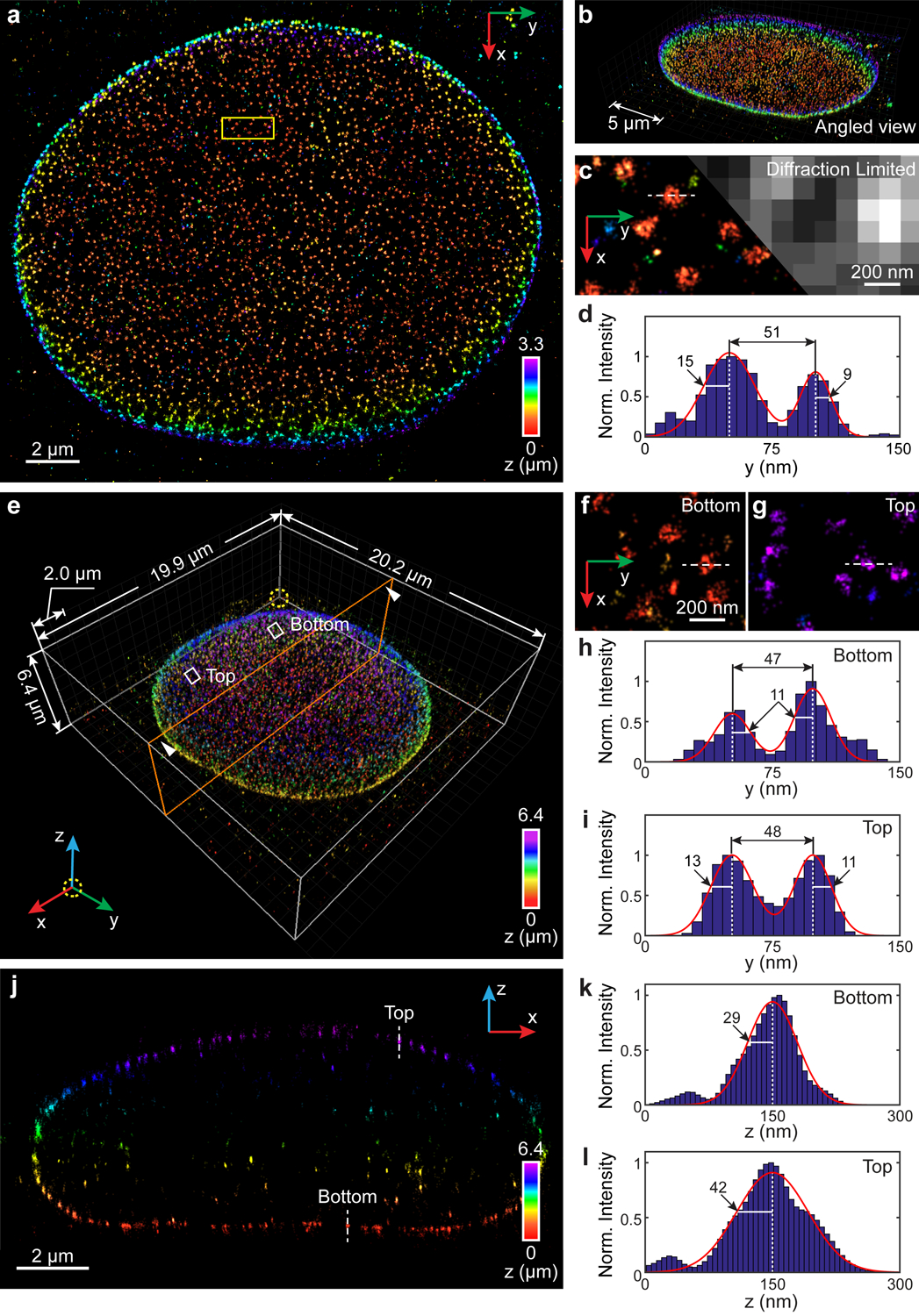
Fig. 4.
3D super-resolution reconstruction of immunofluorescence-labeled Nup98 on the nuclear envelope in COS-7 cells.
(a) x-y overview of a 3.3-u03bcm-thick volume of thennucleus. (b) Angled view of (a). (c) Sub-region asnindicated by the yellow boxed region in (a) showing the ultra-structure of Nup98n(left), which i...
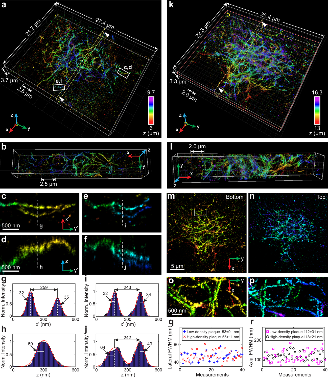
Fig. 5.
3D super-resolution reconstruction of immunofluorescence-labeled amyloid u03b2 (Au03b2) plaques in 30-u03bcm-thick brain sections from an 8-month-old 5XFAD mouse.
(a) Overview of an Au03b2 plaque with low-densitynfibrils. An animated 3D reconstruction is shown in Supplementary Video 6 . (b) Cross section along the yellow plane in (a). (cu2013f) Enlarged yu2019-...
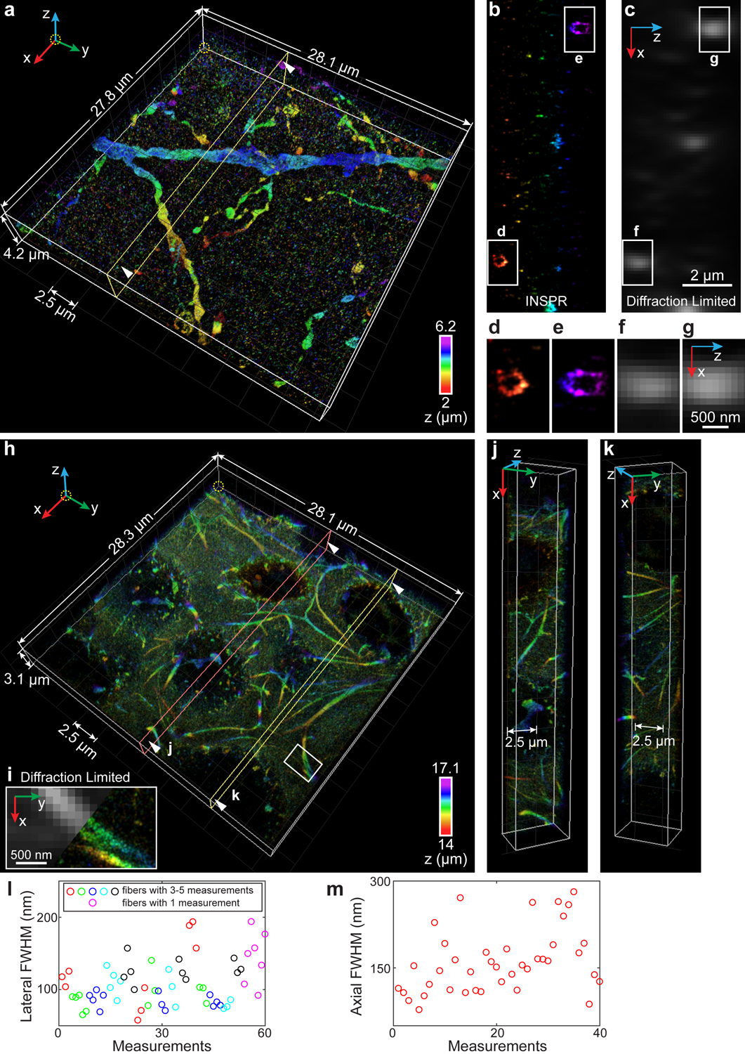
Fig. 6.
3D super-resolution reconstructions of immunofluorescence-labeled ChR2-EYFP on dendrites in visual cortical circuits and immunofluorescence-labeled elastic fibers in developing cartilage.
(a) 3D overview of a 4.2-u03bcm-thick super-resolutionnvolume in a 50-u03bcm-thick brain section labeling ChR2-EYFP. An animated 3Dnreconstruction is shown in Supplementary Video 8 . (b) Axial cross s...
Figure images are served from the NIH/NLM PubMed Central Open Access Subset or Europe PMC; copyright remains with the publishers and authors.
💬 Discussion
0 commentsNo comments yet. Be the first to start a discussion!
Leave a Comment