Abstract
Abstract Motor behavior results in complex exchanges of motor and sensory information across cortical regions. Therefore, fully understanding the cerebral cortex’s role in motor behavior requires a mesoscopic-level description of the cortical regions engaged, their functional interactions, and how these functional interactions change with behavioral state. Mesoscopic Ca2+ imaging through transparent polymer skulls in mice reveals elevated activation of the dorsal cerebral cortex during locomotion. Using the correlations between the time series of Ca2+ fluorescence from 28 regions (nodes) obtained using spatial independent component analysis (sICA), we examined the changes in functional connectivity of the cortex from rest to locomotion with a goal of understanding the changes to the cortical functional state that facilitate locomotion. Both the transitions from rest to locomotion and from locomotion to rest show marked increases in correlation among most nodes. However, once a steady state of continued locomotion is reached, many nodes, including primary motor and somatosensory nodes, show decreases in correlations, while retrosplenial and the most anterior nodes of the secondary motor cortex show increases. These results highlight the changes in functional connectivity in the cerebral cortex, representing a series of changes in the cortical state from rest to locomotion and on return to rest.
🔬 Techniques
💻 Software
✨ Fluorophores
🧪 Sample Preparation
🏭 Microscope Brands
📷 Detectors
🎨 Filters
💻 Software Details
💾 Data Repositories
🏛️ Research Organizations (ROR)
Affiliated research institutions:
📋 Methods
All animal studies were approved by and conducted in conformity with the Institutional Animal Care and Use Committee of the University of Minnesota.
Animals and Surgical Procedures
Eight (five male, three female) transgenic mice expressing GCaMP6f primarily in layers II/III and V excitatory pyramidal neurons of the cerebral cortex (C57BL/6J, Thy1-GCaMP6f Jackson Laboratories JAX 024339) were used ( Dana et al. 2014 ). To obtain optical access to a large region of the dorsal cerebral cortex, we implanted morphologically conformant windows made from transparent polymer ( Ghanbari et al. 2019 ). Prior to surgery, animals were administered slow-release buprenorphine (2 mg/kg, subcutaneous injection) and then anesthetized with isoflurane (5% induction, 0.5–3% maintenance). The head was shaved and mounted in a stereotaxic frame that did not damage the auditory meatus. Depth of anesthesia was monitored by toe pinch response every 15 min. Isoflurane levels were adjusted with respiration rate or if a response to pain was registered. Body temperature was maintained (37°C) using a feedback-controlled heating pad, and the corneas were protected with eye ointment. The surgical procedure began with excision of the scalp, followed by removal of the fascia so that the positions of lambda and bregma could be recorded. High-resolution images with a reference scale were captured both before and after securing the implant to the skull using a digital microscope camera (S01-0801A, Science Supply) attached to the surgical microscope to identify bregma after removing the skull. A manual craniotomy removed a flap of skull that matched the geometry of the implant window, leaving the dura intact. The implant was aligned to the craniotomy and fixed to the skull using a bone screw (F000CE094, Morris Precision Screws and Parts) placed 2–3 mm posterior to lambda. The implant periphery was glued to the skull (Vetbond, 3M) and cemented in place with dental cement (S380 S&B Metabond, Parkell Inc.). Following the cure of the cement, a custom, head-fixing titanium frame was fastened to the implant using three screws (3/32″ flat head 0–80). A second application of dental cement enclosed the fastening screws. After surgery, the mice recovered to an ambulatory state on a heating pad and then were returned to a clean home cage. Mice were administered meloxicam (2 mg/kg, s.c.) for three days and allowed a minimum of seven days to recover before any experimental procedures were initiated.
Show full methods section
All animal studies were approved by and conducted in conformity with the Institutional Animal Care and Use Committee of the University of Minnesota.
Animals and Surgical Procedures
Eight (five male, three female) transgenic mice expressing GCaMP6f primarily in layers II/III and V excitatory pyramidal neurons of the cerebral cortex (C57BL/6J, Thy1-GCaMP6f Jackson Laboratories JAX 024339) were used ( Dana et al. 2014 ). To obtain optical access to a large region of the dorsal cerebral cortex, we implanted morphologically conformant windows made from transparent polymer ( Ghanbari et al. 2019 ). Prior to surgery, animals were administered slow-release buprenorphine (2 mg/kg, subcutaneous injection) and then anesthetized with isoflurane (5% induction, 0.5–3% maintenance). The head was shaved and mounted in a stereotaxic frame that did not damage the auditory meatus. Depth of anesthesia was monitored by toe pinch response every 15 min. Isoflurane levels were adjusted with respiration rate or if a response to pain was registered. Body temperature was maintained (37°C) using a feedback-controlled heating pad, and the corneas were protected with eye ointment. The surgical procedure began with excision of the scalp, followed by removal of the fascia so that the positions of lambda and bregma could be recorded. High-resolution images with a reference scale were captured both before and after securing the implant to the skull using a digital microscope camera (S01-0801A, Science Supply) attached to the surgical microscope to identify bregma after removing the skull. A manual craniotomy removed a flap of skull that matched the geometry of the implant window, leaving the dura intact. The implant was aligned to the craniotomy and fixed to the skull using a bone screw (F000CE094, Morris Precision Screws and Parts) placed 2–3 mm posterior to lambda. The implant periphery was glued to the skull (Vetbond, 3M) and cemented in place with dental cement (S380 S&B Metabond, Parkell Inc.). Following the cure of the cement, a custom, head-fixing titanium frame was fastened to the implant using three screws (3/32″ flat head 0–80). A second application of dental cement enclosed the fastening screws. After surgery, the mice recovered to an ambulatory state on a heating pad and then were returned to a clean home cage. Mice were administered meloxicam (2 mg/kg, s.c.) for three days and allowed a minimum of seven days to recover before any experimental procedures were initiated.
Behavioral Setup
Mice were housed in a reversed light–dark (12 h–12 h) room with experiments performed during the dark period, which is the normal waking and high activity phase of the circadian cycle in mice. After recovery from surgery, polymer window-implanted mice were habituated to the behavioral setup in increasing time increments (5 min, 15 min, 40 min, 1 h) before experiments began. For the behavioral setup, mice were head-fixed on a low-friction, horizontal disk treadmill that allowed for natural movements such as walking and grooming ( Fig. 1 A ). Once habituated, animals alternated between periods of awake quiescence (i.e., rest) and spontaneous walking, which were used for spontaneous locomotion analysis. To offset any potential effects created by the mildly curved path of the disk treadmill, a subset (22 of 62) of experimental sessions were recorded with the mouse head-fixed to the disk pointing in the opposite direction. A high-speed, IR-sensitive CMOS camera (Flea3, Point Grey) recorded the limb and body movements at 40 Hz throughout a session, under diffuse infrared light that did not interfere with the Ca 2+ imaging. Behavioral videos were recorded using Spinnaker SDK software (FLIR Systems). Figure 1 Mesoscopic cortical recording setup and activity during locomotion. ( A ) Experimental setup for behavioral and Ca 2+ fluorescence imaging of head-fixed mice. ( B ) Approximate cortical regions, as defined by the Allen Brain Atlas Common Coordinate Framework ( Allen Institute for Brain Science 2015 ), observable through the polymer skull (inset) by epifluorescence microscopy. Scale bar = 1 mm. Common Framework colors correspond to cortical regions defined in key. ( C ) Treadmill velocity (bottom, blue line) is plotted for an example of spontaneous locomotion in a single mouse. Preprocessed maps of cortical activity (top) shown as mean subtracted % change in fluorescence (∆ F / F ). For visualization only, frames were spatially filtered with a 3 × 3 moving mean and averaged across five frames. Gray dashed lines link maps of cortical Ca 2+ fluorescence with time points prior to, during, and after locomotion. ( D ) Markers used to track paw positions during periods of rest and locomotion for this example data. Blue, front left paw (FL); red, front right paw (FR); orange, hind left paw (HL). ( E ) Horizontal (top) and vertical (bottom) paw displacements versus time during rest. ( F ) Horizontal (top) and vertical (bottom) paw displacements versus time during locomotion. Maximum displacement of each paw (inset, arrows) shows stereotypic, repeating step-cycles. Locomotion kinematics were calculated from the treadmill angular displacement as measured by a high-resolution rotary encoder and recorded by an Arduino Uno microcontroller (Arduino) at 1 kHz. Velocity was determined and smoothed using a sliding average (100 ms window, 1-ms step size). Locomotion was defined as periods of movement in which the wheel reached a velocity of 0.25 cm/s or greater. Working back from 0.25 cm/s, movement onset was then defined as the time wheel velocity first exceeded 0 cm/s, and movement offset was defined as the time velocity returned to 0 cm/s. Periods in which velocity remained between −0.25 and 0.05 cm/s were labeled as rest, while all remaining periods were discarded as “fidgeting” or backwards walking. During rest, visual observation confirmed that the mice were awake but quiet. The horizontal and vertical positions of all four paws were tracked and extracted from the behavioral camera recordings using DeepLabCut behavior tracking software ( Mathis et al. 2018 ). The position of the left forepaw was chosen for further analysis as it was the most visible in the behavioral camera’s field of view and most accurately tracked. The other paws were not included in the final results because of lower quality tracking data and because their movements are highly correlated to the left forepaw, therefore not providing additional information to the regression analysis of the fluorescence data with forepaw velocity (see below). Paw position was only included in further analysis if the DeepLabCut tracking was of high quality (confidence >70%). The horizontal and vertical velocities were calculated as the absolute change in pixels over time and down sampled to 20 fps to align with fluorescence data. Total paw velocity was calculated as the magnitude of the vector sum of the horizontal and vertical velocities. Note that as the view of the infrared camera was not perfectly parallel to the main axis of paw motion, this measure of velocity will not be exact and should be considered an estimate of paw velocity.
Fluorescence Imaging
Head-fixed mice were placed on the treadmill beneath a Nikon AZ-100 microscope ( Fig. 1 A ). Single-photon fluorescence imaging was performed using a high-speed, electron multiplying CCD (Andor, iXon3) controlled with MetaMorph (Molecular Devices Inc.). A filter set with 480/20 nm excitation, 505 nm dichroic, and 535/25 nm emission filters was used (Chroma). Using the variable magnification function, the field-of-view was adjusted to image the exposed dorsal cortical surface (6.2 mm × 6.2 mm) with a spatial resolution of 256 × 256 pixels (pixel size of ~24.2 μm × 24.2 μm). Images were acquired at 20 Hz, 20 ms exposure, for 5 min (6000 frames), and 12 imaging trials were obtained in a session (i.e., the number of trials obtained in 1 day). Time between imaging trials ranged between 1 and 5 min. As the imaging modality was single-photon, the Ca 2+ fluorescence signals are primarily from the excitatory neuronal activity in layers II/III ( Yizhar et al. 2011 ; Ma et al. 2016 ; Waters 2020 ). Fluorescence Imaging Analysis The Ca 2+ fluorescence data from each imaging session was spatially registered using affine transformations. Consistent points on the visible blood vessels in the brain were manually selected and aligned using the built-in MATLAB function, fitgeotrans , with the “affine” method selected. All sessions were registered to the same representative session for a mouse. To remove motion artifacts within trials, all frames were registered to subpixel precision using the dftregistration MATLAB function ( Guizar-Sicairos et al. 2008 ). To remove artifacts potentially introduced through increased overall fluorescence or through blood flow and blood vessel constriction or dilation, masks were drawn over representative sections of background and blood vessels. The mean activity was taken from each of these masks, and the activity of each pixel was regressed against these traces. Only the residuals from these regressions were kept for further analysis, thus removing from the fluorescence signals contributions of background fluorescence and blood flow. To reduce the dimensions of the data to a manageable level and decrease noise, we performed spatial independent component analysis (sICA) to identify a catalog of functionally relevant cortical regions. For each mouse, images from all trials were concatenated and compressed using singular value decomposition (SVD). Only the first 200 singular values were used to recreate the spatial dimension of the data ( Musall et al. 2019 ). We computed the first 50 spatial independent components (ICs) using the Joint Approximation Diagonalization of Eigenmatrices (JADE) algorithm that decomposes mixed signals into ICs by minimizing the mutual information with a series of Givens rotations ( Cardoso 1999 ; Makino et al. 2017 ; Sahonero-Alvarez and Calderon 2017 ). This method provides a blind segmentation of the cerebral cortex based only on statistical properties of the Ca 2+ activity and does not use any prior assumptions regarding cerebral function or architecture. Masks of ICs were made by setting intensity values below 3.5 equal to 0. Masks covering less than 150 contiguous pixels or that, upon visual inspection, corresponded to artifacts not associated with cortical activity were discarded. This included vascular artifacts that survived the regression step above. An IC that included multiple discontinuous areas, such as homotopic cortical regions, was separated into individual ICs, and these individual ICs were used in subsequent analyses. All remaining IC masks were visually inspected, and any remaining area corresponding to blood vessels that were not separated from cortical activity were manually identified and removed. To group data across animals, ICs in each mouse catalog were manually assigned to 1 of 28 nodes of interest (14 per hemisphere) that were present in the majority of mice and corresponded, approximately, to known cortical regions based on the Common Coordinate Framework ( Fig. 2 ) ( Allen Institute for Brain Science 2015 ). Figure 2 Spatial segmentation of the dorsal cerebral cortex using sICA. ( A ) Fifteen ICs representing cortical activity from mouse 1 calculated using JADE ICA, before thresholding and manual artifact removal. ( B ) IC catalogs of each mouse after thresholding and manual artifact removal. Color corresponds to the node identity assigned to each one of the 28 common ICs found across mice as shown in C . ( C ) Locations of the 28 common ICs that define the network nodes observed across mice mapped onto the Common Coordinate Framework ( Allen Institute for Brain Science 2015 ). Behavior Periods Recordings were divided into six behavior periods, each 3 s in duration, as defined by treadmill velocity (see Figs 3 B and 4 A ): 1) rest (see definition above); 2) prelocomotion (rest just prior to locomotion onset; “prep.”); 3) initiation of locomotion (locomotion just after locomotion onset; “init.”); 4) continued locomotion (periods of steady-state, continued locomotion outside of transition periods; “cont.”); 5) termination of locomotion (locomotion just prior to locomotion offset; “term.”); and 6) postlocomotion (rest just after locomotion offset; “after”). Periods of rest or continued locomotion that lasted longer than 3 s were divided into multiple 3-s segments, and remainder data at the end of the period was removed. Periods less than 3 s were also removed. We chose 3-s periods (60 time points) because this provides sufficient data to calculate robust Pearson correlations on the associated fluorescence time series for the functional connectivity analysis (see below). For the subsequent analyses (linear regression, functional connectivity, and Granger causality) of the fluorescence signals, all computations are based on the data from the individual 3-s periods, followed by averaging of the results for each behavior period. Figure 3 Fluorescence activity (∆F/F) within ICs across behavior periods. ( A ) IC catalog of mouse 3, as shown in Figure 2B . ( B ) Top: Example fluorescence time series from each IC for a single bout of locomotion in mouse 3, with the timeline of five of the six behavior periods on top. Bottom: corresponding treadmill activity. ( C ) Top: Fluorescence activity from the common set of 28 nodes averaged over all mice and across all instances of each 3-s behavior period ( n = number of periods averaged). Abbreviations: pre., prelocomotion; initiate., initiation of locomotion; continued, continued locomotion; term., termination of locomotion; after, after locomotion. Bottom: Mean (black lines) and SD (red lines) of treadmill velocity across each behavior time period for all mice. Figure 4 Average results of node fluorescence activity regressions against treadmill velocity ( A and B ) and velocity of the left front paw ( C and D ). ( A ) Average R 2 of regressions of fluorescence activity against treadmill velocity for each behavior period. ( B ) Percent of regressions preformed for each 3-s period in A that reach significance. ( C ) Average R 2 of fluorescence regressions activity against the velocity of the front left paw in each behavior period. ( D ) Percent of regressions in C that reach significance. Regression of Fluorescence Activity against Treadmill and Paw Velocity The masks from the IC catalog for each mouse were used to extract mean fluorescence time series (based on the preprocessed series of image data) for each 5-min trials. The resulting time series were linearly detrended and divided into individual 3-s behavior periods. To determine how fluorescence activity in each node modulated with the parameters of locomotion, linear models were used to regress the fluorescence activity of each node to the treadmill velocity and to the velocity of the left forepaw. Because brain activity and behavior are not necessarily aligned in time, the velocity of the treadmill and left paw were shifted in time relative to the fluorescence activity and included in the regression models as independent predictors (see Fig. 4 ). Shifts in time (“lags”) extended from 500 ms before fluorescence activity to 1.0 s after, in intervals of 100 ms, for a total of 16 predictors in a regression, plus an intercept predictor. Note that, since the fluorescence activity is assigned to a specific 3-s behavior period and does not vary in time, velocity from before or after the behavior period is included in the regression (i.e., the preparation period fluorescence will be regressed to treadmill velocity from up to 1.0 s of the initiation period). Separate regressions were also performed for each lag individually ( Supplementary Fig. 1 ) to clarify how fluorescence activity and behavior are related in time. The R 2 values and statistical significance ( F -test, α < 0.05) were calculated for each instance of a behavior. The R 2 values were averaged for each behavior period over all trials and then across animals. All regressions were calculated using the MATLAB built-in regress function.
Functional Connectivity Analysis
For each 3-s period, the correlation coefficients (ρ) were calculated between the time series from all catalog ICs to generate a correlation (i.e., adjacency) matrix, and the matrices obtained from each 3-s period were averaged to create mean adjacency matrices for each behavior period per mouse. To combine data across animals, the averaged correlations were assigned to the appropriate corresponding node. If more than one catalog IC had been assigned to a node, then the correlation values of those catalog ICs were averaged. The mean adjacency matrices were then averaged across the subjects. For each pair of regions, the significant change in correlation of activity between behavior periods was calculated using custom MATLAB code. The difference in correlation was compared with a null distribution of differences from 500 reshufflings of the correlations across behavior. Significance was determined by α < 0.05 corrected with the false discovery rate ( Genovese et al. 2002 ). To further quantify the functional relationships between brain regions during locomotion, the network centrality of ICs was calculated on 3-s correlation matrices using MATLAB code from the Brain Connectivity Toolbox ( Rubinov and Sporns 2010 ). The eigenvector centrality was calculated from the correlation adjacency matrices for each 3-s period and averaged within each mouse before being averaged across mice. Similar to the comparisons among the correlations between regions, the difference in eigenvector centrality for each region from one period to another was compared with a null distribution of differences from 500 reshufflings of the centralities across behavior. Again, significance was determined by α < 0.05 corrected with the false discovery rate. Since it is possible that large, global increases or decreases in fluorescence activity could increase correlation coefficients between nodes and obscure more subtle changes in connectivity, an additional analysis was performed in which low-frequency changes in fluorescence activity were removed using a 5 th order high-pass Butterworth filter with a cutoff filter of 2 Hz. The filter was applied to the mean fluorescence time series extracted from the IC masks for each mouse. Correlation and eigenvector centrality calculations were repeated on the filtered data as described above.
Granger Causality Analysis
Granger causality among the nodes was determined as a measure of the directional influence between cortical regions during different behavior periods. We used the Multivariate Granger Causality MATLAB Toolbox ( Barnett and Seth 2014 ), with the ordinary least squares model estimation and regression information criteria and the Akaike information criterion (AIC) model order. The model was limited to a maximum of 20 lags. For each animal, the time series from all instances of a 3-s behavior period were inputted to the algorithm as separate trials to generate a single, multivariate causality adjacency matrix for each mouse. These individual adjacency matrices were averaged across mice as described above. Granger causality estimates the causality between time series in both directions. In order to have a single directional value representing the net relationship between two regions, a “total causality” value was calculated based on the difference in magnitude of the corresponding causalities. In adjacency matrices, total causality direction is indicated as a positive or negative value. Significant changes in causality between behavior periods were determined similar to the approach used for significant changes in correlation and centrality. The difference in causality and total causality from one period to another between each pair of ICs was compared with a null distribution of differences from 500 reshufflings of the causalities across behavior. Significance was determined by α < 0.05 corrected with the false discovery rate.
Hemodynamic Correction
Blood flow increases with neuronal activation, and oxygenated blood absorbs light with peak absorption at ~530 nm, decreasing the duration of the increased GCaMP fluorescence ( Ma et al. 2016 ). Therefore, additional experiments were performed to evaluate the effects of hemodynamics and other Ca 2+ -independent fluorescence changes such as flavoprotein autofluorescence ( Vanni and Murphy 2014 ; Jacobs et al. 2020 ), using three mice (one from the original cohort and two additional). Data were collected in 5-min stacks, similar to the primary dataset. Data were collected in 36 stacks across 3 recording days for mouse #8, 35 stacks across 8 days for mouse #9, and 68 stacks across 12 days for mouse #10, for a total of 11.58 hours of data. We used dual-wavelength illumination to capture both Ca 2+ -dependent (470 nm, blue light) and Ca 2+ -independent (405 nm, violet light) GCaMP6f signals on consecutive frames using a Cairn OptoLED driver (Cairn OptoLED, P1110/002/000; P1105/405/LED, P1105/470/LED) ( Ma et al. 2016 ; Allen et al. 2017 ; Jacobs et al. 2020 ; Musall et al. 2019 ; MacDowell and Buschman 2020 ). An excitation filter (ET480/40, Chroma) was placed in front of the 470 nm LED and then both light sources were combined into the parallel light path of a Nikon AZ100M macroscope through a dichroic mirror (425 nm, Chroma T425lpxr), which was reflected off a second dichroic (505 nm, Chroma T505pxl) to the brain. Cortical GCaMP6f emissions then passed back through the second dichroic into an sCMOS camera (Andor Zyla 4.2 Oxford Instruments). Exposure times for each frame were 18 ms, synced via TTL pulses from a Cambridge Electronics 1401 (Cambridge Electronic Design Limited) acquisition system that controlled both LEDs and the external trigger of the Andor Zyla 4.2. Frames were captured at 40 Hz (20 Hz per channel) at 256 × 256 pixels per image. Using a previously described correction method ( Ma et al. 2016 ; Jacobs et al. 2020 ; MacDowell and Buschman 2020 ), the Ca 2+ -independent signals were removed by first calculating the per-pixel average intensity in both channels and then scaling the 405-nm channel to a similar level of the 470-nm channel by multiplying by the ratio of the per-pixel averages. The scaled 405-nm signal was then subtracted from the 470-nm signal and the resulting signal was then normalized by dividing by the scaled 405-nm signal. All subsequent processing, including sICA, functional connectivity, and network measures, was identical to that preformed on the mono-wavelength, uncorrected data. All MATLAB analysis codes for sICA segmentation of mesoscale Ca 2+ imaging, eigenvector centrality, and hemodynamic correction are available upon request .
Animals and Surgical Procedures
Eight (five male, three female) transgenic mice expressing GCaMP6f primarily in layers II/III and V excitatory pyramidal neurons of the cerebral cortex (C57BL/6J, Thy1-GCaMP6f Jackson Laboratories JAX 024339) were used ( Dana et al. 2014 ). To obtain optical access to a large region of the dorsal cerebral cortex, we implanted morphologically conformant windows made from transparent polymer ( Ghanbari et al. 2019 ). Prior to surgery, animals were administered slow-release buprenorphine (2 mg/kg, subcutaneous injection) and then anesthetized with isoflurane (5% induction, 0.5–3% maintenance). The head was shaved and mounted in a stereotaxic frame that did not damage the auditory meatus. Depth of anesthesia was monitored by toe pinch response every 15 min. Isoflurane levels were adjusted with respiration rate or if a response to pain was registered. Body temperature was maintained (37°C) using a feedback-controlled heating pad, and the corneas were protected with eye ointment. The surgical procedure began with excision of the scalp, followed by removal of the fascia so that the positions of lambda and bregma could be recorded. High-resolution images with a reference scale were captured both before and after securing the implant to the skull using a digital microscope camera (S01-0801A, Science Supply) attached to the surgical microscope to identify bregma after removing the skull. A manual craniotomy removed a flap of skull that matched the geometry of the implant window, leaving the dura intact. The implant was aligned to the craniotomy and fixed to the skull using a bone screw (F000CE094, Morris Precision Screws and Parts) placed 2–3 mm posterior to lambda. The implant periphery was glued to the skull (Vetbond, 3M) and cemented in place with dental cement (S380 S&B Metabond, Parkell Inc.). Following the cure of the cement, a custom, head-fixing titanium frame was fastened to the implant using three screws (3/32″ flat head 0–80). A second application of dental cement enclosed the fastening screws. After surgery, the mice recovered to an ambulatory state on a heating pad and then were returned to a clean home cage. Mice were administered meloxicam (2 mg/kg, s.c.) for three days and allowed a minimum of seven days to recover before any experimental procedures were initiated.
Supplementary Material Supplementary_figures_and_legends_bhab373 Click here for additional data file.
📊 Figures
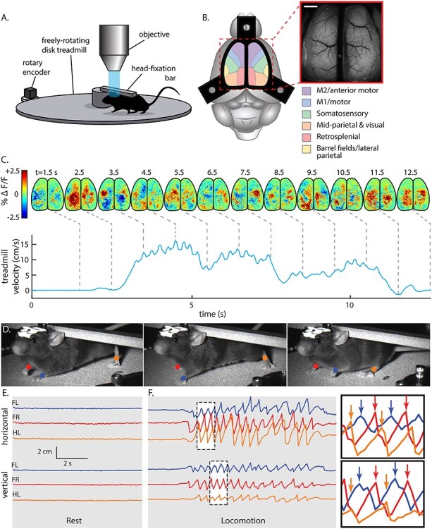
Figure 1
Mesoscopic cortical recording setup and activity during locomotion. ( A ) Experimental setup for behavioral and Ca 2+ fluorescence imaging of head-fixed mice. ( B ) Approximate cortical regions, as de...
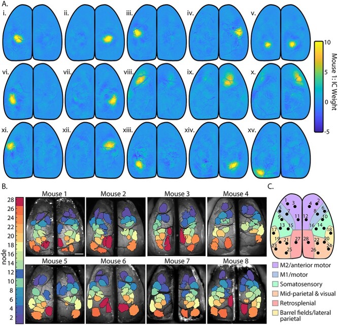
Figure 2
Spatial segmentation of the dorsal cerebral cortex using sICA. ( A ) Fifteen ICs representing cortical activity from mouse 1 calculated using JADE ICA, before thresholding and manual artifact removal....
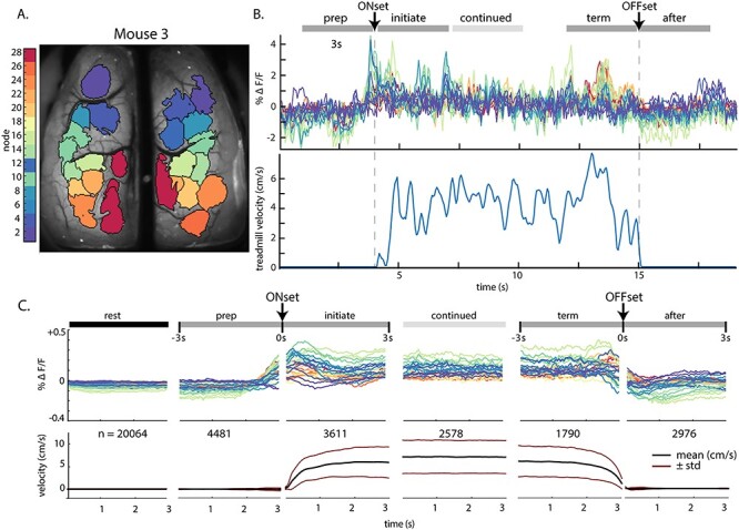
Figure 3
Fluorescence activity (u2206F/F) within ICs across behavior periods. ( A ) IC catalog of mouse 3, as shown in Figure 2B . ( B ) Top: Example fluorescence time series from each IC for a single bout of ...
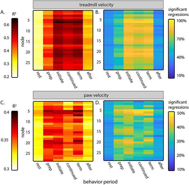
Figure 4
Average results of node fluorescence activity regressions against treadmill velocity ( A and B ) and velocity of the left front paw ( C and D ). ( A ) Average R 2 of regressions of fluorescence activi...
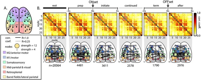
Figure 5
Functional connectivity among the common cortical nodes during behavior periods across all mice. ( A ) Diagram of nodes common to the catalog ICs across mice mapped onto the Common Coordinate Framewor...
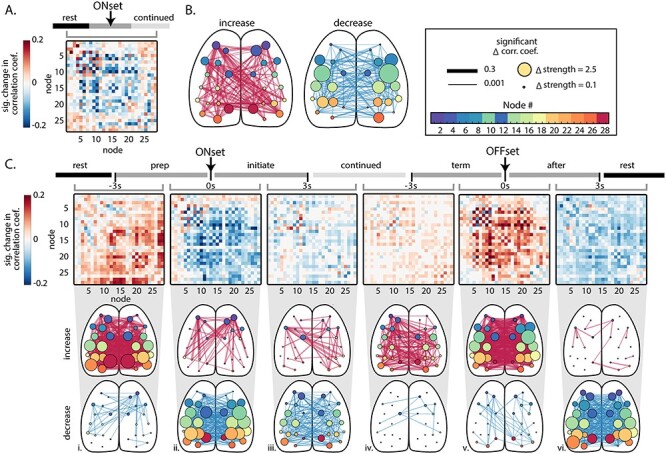
Figure 6
Significant changes in correlations between nodes across behavior periods . ( A ) Matrix of significant changes in correlation between nodes comparing rest to continued locomotion (u03b1u2009<u2009...
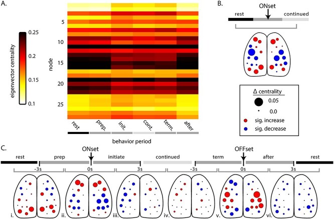
Figure 7
Eigenvector centrality across behavior periods. ( A ) Average eigenvector centrality for each node during the behavior periods, across mice. ( B ) Significant change in centrality comparing rest to co...
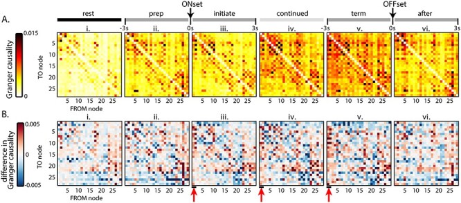
Figure 8
Granger causality between nodes during the behavior periods. In these plots, rows represent the TO node Granger causality, and columns represent the FROM node causality. ( A ) Average Grainger causali...
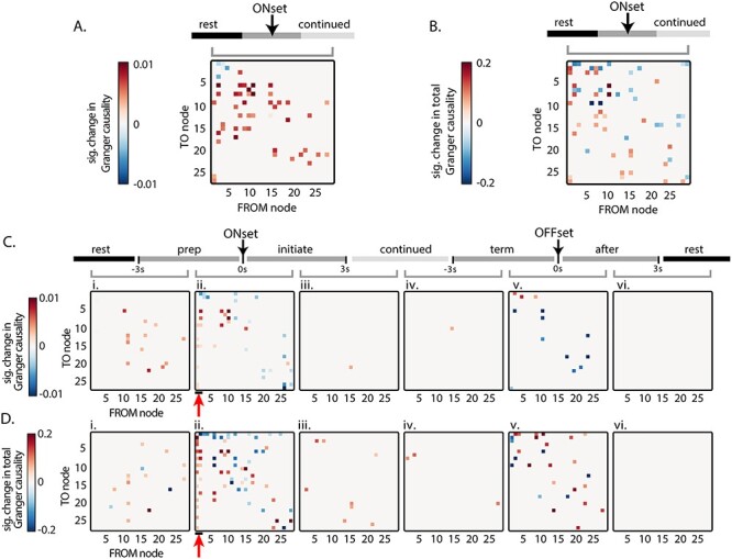
Figure 9
Significant changes in Granger causality between nodes across behavior periods. In these plots, rows represent the TO node Granger causality, and columns represent the FROM node causality. ( A ) Signi...
Figure images are served from the NIH/NLM PubMed Central Open Access Subset or Europe PMC; copyright remains with the publishers and authors.
💬 Discussion
0 commentsNo comments yet. Be the first to start a discussion!
Leave a Comment