Abstract
We present a real-time fitter for 3D single-molecule localization microscopy using experimental point spread functions (PSFs) that achieves minimal uncertainty in 3D on any microscope and is compatible with any PSF engineering approach. We used this method to image cellular structures and attained unprecedented image quality for astigmatic PSFs. The fitter compensates for most optical aberrations and makes accurate 3D super-resolution microscopy broadly accessible, even on standard microscopes without dedicated 3D optics.
🔬 Techniques
🔭 Microscopes
💻 Software
✨ Fluorophores
🧪 Sample Preparation
🔬 Cell Lines
🏭 Microscope Brands
🧪 Reagent Suppliers
📷 Detectors
🎨 Filters
💻 Software Details
💻 Code & Software
💾 Data Repositories
🏛️ Research Organizations (ROR)
Affiliated research institutions:
📋 Methods
Robust averaging of experimental bead stacks Stacks of beads, immobilized on a coverslip, were acquired in a range of ±1000 nm with respect to the coverslip. A spacing in z between 10 nm and 50 nm works well. Beads in each stack were segmented in a maximum intensity projected image by maximum finding and thresholding. Sub regions around each bead location were cropped. Next, we aligned all beads with sub-pixel accuracy by 3D cross-correlation using a single bead as reference. To gain precision, another round of 3D alignment of the central part of each stack was performed using the average of the aligned bead stacks as the reference. We scaled up the central part of the cross-correlation by a factor of 20 by cubic spline interpolation and determined the x, y, and z shifts from the position of the maximum 26 . The bead stacks were shifted using cubic spline interpolation. Iteratively, bead stacks which showed a large dissimilarity from the average were identified based on the maximum value of the cross-correlation and the mean square error and excluded from the average. To eliminate the background, the minimum value of the bead stack was subtracted and the amplitude was normalized by the total (summed up) intensity of the central slice. We further regularized the bead stack by smoothing it in the z-direction with a smoothing B-spline 27 . In the presence of field-dependent aberrations, systematic fitting errors can be corrected in a post-processing step based on a precise calibration 28 . In presence of strong field-dependent aberrations, we suggest to perform the calibration and fitting only locally on small sub-regions of near uniform aberrations.
Show full methods section
Robust averaging of experimental bead stacks Stacks of beads, immobilized on a coverslip, were acquired in a range of ±1000 nm with respect to the coverslip. A spacing in z between 10 nm and 50 nm works well. Beads in each stack were segmented in a maximum intensity projected image by maximum finding and thresholding. Sub regions around each bead location were cropped. Next, we aligned all beads with sub-pixel accuracy by 3D cross-correlation using a single bead as reference. To gain precision, another round of 3D alignment of the central part of each stack was performed using the average of the aligned bead stacks as the reference. We scaled up the central part of the cross-correlation by a factor of 20 by cubic spline interpolation and determined the x, y, and z shifts from the position of the maximum 26 . The bead stacks were shifted using cubic spline interpolation. Iteratively, bead stacks which showed a large dissimilarity from the average were identified based on the maximum value of the cross-correlation and the mean square error and excluded from the average. To eliminate the background, the minimum value of the bead stack was subtracted and the amplitude was normalized by the total (summed up) intensity of the central slice. We further regularized the bead stack by smoothing it in the z-direction with a smoothing B-spline 27 . In the presence of field-dependent aberrations, systematic fitting errors can be corrected in a post-processing step based on a precise calibration 28 . In presence of strong field-dependent aberrations, we suggest to perform the calibration and fitting only locally on small sub-regions of near uniform aberrations.
Calculation of cspline-interpolated PSFs
Spline functions are piecewise polynomials for which high order derivatives are continuous at the knots, where the pieces connect. Cubic splines are the most commonly used splines, e.g. in computer graphics, geometric modeling, etc. Recently, this type of approximation theory has also been used for single molecule localization 10 , 12 , 13 . We implemented the cspline interpolation both in terms of cubic splines and cubic B-splines. A B-spline interpolation is generally less memory intensive since only one B-spline coefficient is needed in each spline interval. In comparison, ( d + 1) n coefficients are required in each spline interval for spline polynomials, where d is the spline degree and n is the dimension. However, our implementation of a 3D fit based on cubic splines is about 2.5 times faster than the cubic B-spline form due to the fact that cubic splines are more explicit and less calculations are needed to calculate spline values and derivatives. Therefore, the software used in this work is based on cubic splines with 64 coefficients in each voxel of the 3D PSF stack. Similar to Ref. 13 , the 3D PSF is described by a three dimensional cubic spline for voxel ( i , j , k ) as follows: f i , j , k ( x , y , z ) = ∑ m = 0 3 ∑ n = 0 3 ∑ p = 0 3 a i , j , k , m , n , p ( x - x i Δ x ) m ( y - y j Δ y ) n ( z - z k Δ z ) p , ( x , y , z ) ∈ R 3 , where Δ x and Δ y is the pixel size of the PSF in the object space in x and y directions, respectively. Δ z is the step size in the objective space in z direction. x i , y j and z k are the start positions of voxel ( i , j , k ) in x , y and z directions, respectively. In order to calculate the cspline coefficients, the 3D PSF stack was firstly built by averaging the bead stacks from different fields of view by 3D cross correlation and by regularization, as described above. The spline coefficients were built based on the averaged and smoothed 3D PSF stack. As 64 cspline coefficients are required to describe each voxel, we up sampled (cubic spline interpolation) each voxel 3 times in x , y and z directions, respectively. The 64 up sampled coordinates (including boundary of neighboring voxels) were used to calculate the 64 cspline coefficients. The code to calculate the spline coefficients from bead stacks can be found in the Supplementary Software 1 . z -calibration of astigmatic Gaussian PSF models Our PSF calibration tool also allows extracting z -positions using two widely used algorithms: a) calculate the z -positions directly from the calibrated σ x ( z ) and σ y ( z ) returned by the elliptical Gaussian fit; b) determine the z-positions by directly fitting the single molecules with the calibrated astigmatic Gaussian PSF model 29 . For both calibrations, the bead stacks are fitted with an elliptical Gaussian PSF model and shifted in z according to their true z -positions where σ x ( z ) == σ y ( z ). The outliers are removed based on the root mean error of σ x ( z ) and σ y ( z ) with respect to the average curves. For algorithm a), we calculate dσ 2 ( z ) = σ x ( z ) 2 − σ y ( z ) 2 and interpolate the functional relationship z ( dσ ) 2 by a smoothing cubic B-spline. This B-spline interpolation is then used to directly read out z from dσ 2 . For algorithm b), σ x ( z ) and σ y ( z ) are fitted with a polynomial approximation for the astigmatic Gaussian model: σ x ( z ) = σ 0 x 1 + ( z - γ d ) 2 + A x ( z - γ d ) 3 + B x ( z - γ d ) 4 , σ y ( z ) = σ 0 y 1 + ( z - γ d ) 2 + A y ( z - γ d ) 3 + B y ( z - γ d ) 4 . The parameters σ 0 x , A x , B x , σ 0 y , A y , B y , γ and d are input parameters for the Gaussian fitter, which directly returns the z -coordinates of the fluorophores. We follow the formula in Ref. 25 to calculate the derivatives of the parameters. However, the iterative process was re-implemented using the Levenberg-Marquardt (L-M) algorithm. Newton and Levenberg-Marquardt iterative schemes for MLE Maximum likelihood estimation is the method of choice for fitting data with Poisson statistics 30 . The objective function for MLE is given by 31 : χ mle 2 = 2 ( ∑ k ( μ k - x k ) - ∑ k , x k > 0 x k ln ( μ k / x k ) ) , where μ k is the expected number of photons in pixel k from the model PSF function, x k is the measured number of photons. By minimizing χ mle 2 , we obtain the maximum likelihood for the Poisson process. Methods for nonlinear optimization are usually iterative. For Newton iterative schemes, the search direction Δ θ i of each iteration is given by 25 ∂ 2 χ mle 2 ∂ θ i 2 Δ θ i = - ∂ χ mle 2 ∂ θ i , where θ i is the i -th free fit parameter. However, computing the second derivatives is often quite difficult and can be destabilizing when the model fits badly or is contaminated by outlier points 30 . An alternative method is the L-M algorithm. The L-M algorithm is often used for least squares fitting as it is quick and robust. With relatively simple modifications 31 , the L-M algorithm has also been used to minimize χ mle 2 . In the L-M algorithm, the second derivatives term is neglected and only the first derivatives are used. In the L-M algorithm, the update Δ θ i is given by ( H i , j + λ I ) Δ θ i = J j , where, H i,j is the Hessian matrix without the second partial derivatives term, defined as H i , j = ∑ k ∂ μ k ∂ θ i ∂ μ k ∂ θ j x k μ k 2 , J j is the Jacobian matrix defined as J j = ∑ k ∂ μ k ∂ θ j ( x k - μ k ) μ k , λ is the damping factor, I is a diagonal matrix equal to the diagonal elements of the Hessian matrix. This method is more robust since a damping factor is introduced and the second derivatives do not contribute. This damping factor is increased (multiplied by 10 in this work) if an iteration step does not decrease χ mle 2 or H i,j is not positive definite. GPU Implementation This GPU implementation of the iterative method follows the framework developed for fitting a Gaussian PSF model using a GPU 25 , however using the L-M algorithm. We note that a general framework for L-M fitting on the GPU has been recently published 32 . Unlike previous work for EMCCD and sCMOS noise models 20 , 25 , where the shared memory was used to store the molecule candidate data and readout noise map, we kept the data in the GPU global memory. Each thread is pointed to each molecule candidate and performs all the computations for each molecule candidate. No thread synchronization is required. 64 threads per block were used. The overall speed is about 1.9 times (small window size) to 47.9 times (large window size) faster ( Supplementary Fig. 12 ) than for the original code where shared memory was employed for the sCMOS noise model. We assume that this is due to the compiler optimization where more registers are used and the time for copying data from the global to the shared memory is saved. Both, the CPU based C-code and the GPU based CUDA-code were compiled using Microsoft Visual Studio 2010. The software was called via Matlab (Mathworks) mex files. It was run on a personal computer using an Intel(R) Core(TM) i7-5930 processor clocked at 3.50 GHz with 64 GB memory. An NVIDIA GeForce GTX 1070 graphics card with 8.0 GB memory was used for GPU based computation.
Simulation of realistic single molecule data
To simulate single molecule images using a realistic PSF model, we used the cspline-interpolated PSF model generated from experimental bead stacks as described above. We generated the single molecule image from this PSF model at a random 3D position, multiplied it with the number of photons/localization and added a constant background. Finally, we applied Poisson noise to the images. For simulations of sCMOS data, we added a pixel-dependent Gaussian noise. The code to simulate PSFs from the calculated cspline coefficients can be found in the Supplementary Software 1 . MLE fit using an sCMOS camera noise model sCMOS cameras have become more and more attractive for localization microscopy due to their fast data acquisition even for large fields of view, low readout noise and relatively low price. However, their intrinsic pixel-dependent gain, offset and readout noise can create a localization bias, which has to be corrected when localizing the single molecule 20 . Gain g k and offset o k in pixel k can be taken into account when converting the camera image I k ADU in analog digital units (ADU) into photons: I k P = ( I k ADU - o k ) / g k . The readout noise, however, has to be taken into account during the fitting in the noise model and can be calculated from many dark camera images as the pixel-wise variance. Here, we use the same model as proposed by Huang, et al. 20 which approximates the normal distributed readout noise ( var k , in units of photoelectrons) with a Poisson distribution. By adding a pixel-dependent constant, var k , to the measured photoelectrons, one can expect the new value to approximate a Poisson distribution with a mean of u k + var k . Here, u k is the expected photon number in pixel k of the PSF model function. Therefore, in comparison to the conventional MLE fit for EMCCD data, only one more parameter, var k , is required for sCMOS data. Also var k is only kept in the global memory of the GPU. Compared to the EMCCD noise model, the speed performance of the algorithm was only reduced by less than 25% by additionally accounting for the pixel dependent readout noise ( Supplementary Fig. 12 ). 3D Fitting of SMLM data acquired with standard microscopes without 3D optics As our code includes fitting with arbitrary PSFs, it is directly applicable on 2D data, acquired with an unmodified PSF in a standard microscope. A model for the unmodified PSF can be calculated directly from bead stacks, in an analogous way to engineered PSFs. However, the unmodified PSF has a high symmetry with respect to the focal plane ( Supplementary Figure 1 ), making it difficult for an iterative fitting procedure to converge through the focal plane. To overcome this problem, we fit every localization twice: once with a starting parameter for the z -position 500 nm above the focal plane, and once with a starting parameter 500 nm below the focal plane. The maximum likelihood is then used to select the better fit. As a real PSF is not completely symmetric 33 , this breaks the degeneracy previously encountered when extracting z -positions in 2D data sets from only a single photometry or PSF size parameter 18 . Due to the rather large size of the calibration bead (100 nm) and small inaccuracies during the averaging of many bead stacks, the cspline PSF model is slightly blurred compared to a single-molecule PSF. This had no apparent effect on 3D data, but in 2D data it lead to an accumulation of fitted localizations at the focal plane. To overcome this problem, we filtered the raw images with a Gaussian kernel (standard deviation σ < 0.5 pixels), thus applying the blur in the PSF model to the data. To find the right σ , we fitted a subset of the data with several values for σ = 0, 0.1, …, 0.5 and selected the σ value for which we found neither an accumulation nor a depletion of localizations around the focal plane.
Post processing
As the positions used above are all based on the objective positions, which differ from the true absolute positions due to refractive index mismatch, we further multiply the z -positions with a refractive index mismatch factor of 0.75 1 . Then, x , y , and z -positions were corrected for residual drift by a custom algorithm based on redundant cross-correlation. Localizations persistent in consecutive frames were grouped into one localization, and superresolution images were constructed with every localization rendered as a 2D elliptical Gaussian with a width proportional to the localization precision. For measurements deep in the sample in combination with oil objectives, aberrations induced by the refractive index mismatch can be corrected for as described in Ref. 34 .
Sample preparation of clathrin-coated pits in SK-MEL-2 cells
All samples were imaged on round 24 mm high precision glass coverslips No. 1.5H (117640, Marienfeld, Lauda-Königshofen, Germany). Coverslips were cleaned overnight in a 1:1 mixture of concentrated HCl and methanol, rinsed with millipore water until neutral, dried and UV sterilized in a standard cell culture hood. SK-MEL-2 cells (kind gift from David Drubin, described in Ref. 35 ) were cultured under adherent conditions in DMEM/F-12 (Dulbecco’s Modified Eagle Medium/Nutrient Mixture F-12) with GlutaMAX and phenol red (ThermoFisher 10565018) supplemented with 10% [v/v] FBS, ZellShield ™ (Biochrom AG, Berlin, Germany), and 30 mM HEPES at 37°C, 5% CO2 and 100% humidity. Cells were fixed using 3% [w/v] paraformaldehyde (PFA) in cytoskeleton buffer (CB; 10 mM MES pH 6.1, 150 mM NaCl, 5 mM EGTA, 5 mM D-glucose, 5 mM MgCl 2 , described in Ref. 36 ) for 20 minutes. Fixation was stopped by incubation in 0.1% [w/v] NaBH 4 for 7 minutes. The sample was washed with PBS three times, and subsequently permeabilised using 0.01% [w/v] digitonin (Sigma-Aldrich, St. Louis, MO, USA) in PBS for 15 minutes. After washing twice with PBS, the sample was blocked with 2% [w/v] BSA in PBS for 60 minutes, washed again with PBS, and stained for 3–12 hours with anti-clathrin light chain (sc-28276, Santa Cruz Biotechnology, Dallas, TX, USA, diluted 1:300) and anti-clathrin heavy chain rabbit polyclonal antibodies (ab21679, Abcam, Cambridge, UK, diluted 1:500) in 1% [w/v] BSA in PBS. The sample was washed with PBS three times, and incubated with a donkey anti-rabbit secondary antibody (711-005-152, Jackson ImmunoResarch, West Grove, PA, USA), which was previously conjugated with Alexa Fluor 647-NHS at an average degree of labeling of 1.5, for 4 hours. Finally, the sample was washed three times with PBS prior to imaging. For dSTORM imaging, coverslips were mounted in 500 μL blinking buffer (50 mM Tris pH 8, 10 mM NaCl, 10% [w/v] D-glucose, 35 mM 2-mercaptoethylamine (MEA), 500 μg/mL GLOX, 40 μg/mL catalase, 2 mM COT). Sample preparation for imaging of the nuclear pore complex and microtubules Wildtype U-2 OS and genome-edited U-2 OS cells that express Nup107-SNAP (as previously described in Ref. 37 ) were cultured under adherent conditions in Dulbecco’s Modified Eagle Medium (DMEM, high glucose, w/o phenol red) supplemented with 10% [v/v] FBS, 2 mM L-glutamine, non-essential amino acids, ZellShield ™ (Biochrom AG, Berlin, Germany) at 37°C, 5% CO 2 and 100% humidity. All incubations were carried out at room temperature. For nuclear pore staining, the coverslips were rinsed twice with PBS and prefixed with 2.4% [w/v] PFA in PBS for 30 seconds. Cells were permeabilized with 0.4% [v/v] Triton X-100 in PBS for 3 minutes and afterwards fixed with 2.4% [w/v] PFA in PBS for 30 minutes. Subsequently, the fixation reaction was quenched by incubation in 100 mM NH 4 Cl in PBS for 5 minutes. After washing twice with PBS, the samples were blocked with Image-iT ™ FX Signal Enhancer (ThermoFisher Scientific, Waltham, MA, USA) for 30 minutes. The coverslips were incubated in staining solution (1 μM benzylguanine Alexa Fluor 647 (S9136S, NEB, Ipswich, MA, USA); 1 mM DTT; 1% [w/v] BSA; in PBS) for 50 minutes in the dark. After rinsing three times with PBS and washing three times with PBS for 5 minutes, the sample was mounted for imaging. For microtubule staining, wildtype U-2 OS cells were prefixed for 2 minutes with 0.3% [v/v] glutaraldehyde in CB + 0.25% [v/v] Triton X-100 and fixed with 2% [v/v] glutaraldehyde in CB for 10 minutes. Fluorescent background was reduced by incubation with 0.1% [w/v] NaBH 4 in PBS for 7 minutes. After 3 washes with PBS, microtubules were stained using anti alpha-tubulin antibody (MS581, NeoMarkers, Fremont, CA, USA) 1:300 in PBS + 2% [w/v] BSA for 2 h and anti-mouse Alexa Fluor 647 (A21236, Invitrogen, Carlsbad, CA, USA) 1:300 in PBS + 2% [w/v] BSA for 2h. After 3 washes with PBS samples were imaged in a blinking buffer as described above, but with pyranose oxidase instead of glucose oxidase. For DNA-PAINT imaging, microtubules were labelled with anti alpha-tubulin antibodies (MS581, NeoMarkers, and T6074, Sigma-Aldrich, St. Louis, MO, USA) and anti beta-tubulin antibody (T5293, Sigma-Aldrich) each 1:300 diluted in PBS with 2% [w/v] BSA, for 2 hours. After 3 washes with PBS, samples were incubated with a DNA labelled anti-mouse secondary antibody overnight (docking strand sequence: 5′-TT ATA CAT CTA-3′) and imaged after 5 washes with PBS using 50 pM of complementary Atto-655 labelled DNA imager strand (5′-C TAG ATG TAT-3′-Atto655) in PAINT buffer (PBS, 500 mM NaCl, 40 mM Tris, pH 8.0).
Microscopy
SMLM image acquisition was performed at room temperature (24 °C) on a customized microscope 38 equipped with a high NA oil immersion objective (160x, 1.43-NA oil immersion, Leica, Wetzlar, Germany). We employed a laser combiner (LightHub®, Omicron-Laserage Laserprodukte, Dudenhofen, Germany) with Luxx 405, 488 and 638, Cobolt 561 lasers. The lasers were triggered using a FPGA (Mojo, Embedded Micro, Denver, CO, USA) allowing microsecond pulsing control of lasers. After passing through a speckle reducer (LSR-3005-17S-VIS, Optotune, Dietikon, Switzerland), the laser is then guided through a multimode fiber (M105L02S-A, Thorlabs, Newton, NJ, USA). The output of the fiber is first magnified by an achromatic lens and then imaged into the sample 38 . A laser clean-up filter (390/482/563/640 HC Quad, AHF, Tübingen, Germany) is placed in the beam path to remove fiber generated fluorescence. A close-loop focus lock system was implemented using the signal of a near infrared laser reflected by the coverslip and its detection by a quadrant photodiode. The focus can be stabilized within ±10 nm over several hours 39 . The fluorescence emission was filtered by a bandpass filter (700/100, AHF or 676/37, AHF) and recorded by an EMCCD camera (Evolve512D, Photometrics, Tucson, AZ, USA). Typically, we acquire 100,000 – 300,000 frames with 15 ms exposure time (100 ms for DNA-PAINT) and laser power densities of ~15 kW/cm 2 . The pulse length of the 405 nm laser is automatically adjusted to retain a constant number of localizations per frame. Controlled induction of optical aberrations was carried out on a similar microscope, albeit with an additional detection path. After the tube-lens, the back-focal plane of the objective is imaged onto a deformable mirror (Mirao 52e, Imagine Optic, Orsay, France) for phase correction. A flip mirror allows guiding the light either towards a Shack-Hartmann wavefront sensor (HASO3, Imagine Optic) or the camera for fluorescence imaging. The PSFs were obtained by correcting the optical aberrations using a closed loop between the mirror and the wavefront sensor in Casao (Imagine Optic) and image-based optimization of a single-bead in Micao (Imagine Optic). Aberrations were then induced based on pure Zernike modes. Furthermore, SMLM images were acquired on a commercial Leica SR GSD 3D microscope. The setup is equipped with a 500 mW 642 nm laser (MPBC Inc., Montreal, Canada), a 30 mW 405 nm diode laser (Coherent Inc., Santa Clara, CA, USA), a DBP 405/10 642/10 excitation filter, a LP649 dichroic mirror, a BP 710/100 emission filter and a high NA oil immersion objective (160x, 1.43-NA oil immersion, Leica). Astigmatism was induced with a modified tube lens and the image was recorded on an iXon3 897 EMCCD camera (Andor, Belfast, Northern Ireland). Reference images were reconstructed with the Leica Application Suite X (Version 1.9.0.13747) and used as comparison to the cspline fit.
Statistics and reproducibility
All figures show representative data from ≥3 ( Figure 1 , Supplementary Figures 6, 11 ) or ≥5 ( Figure 2 , Supplementary Figures 1 ) representative experiments, or from single experiments ( Supplementary Figure 9, 14, 15 ). Supplementary Figure 13 shows representative data from 3 similar independent simulations.
Code availability
Source code for the software used in this manuscript is contained in Supplementary Software 1 and updated versions can be freely downloaded at github.com/jries/fit3Dcspline.git.
Data availability statement
The datasets generated and analysed during the current study are available from the corresponding author upon reasonable request.
Robust averaging of experimental bead stacks Stacks of beads, immobilized on a coverslip, were acquired in a range of ±1000 nm with respect to the coverslip. A spacing in z between 10 nm and 50 nm works well. Beads in each stack were segmented in a maximum intensity projected image by maximum finding and thresholding. Sub regions around each bead location were cropped. Next, we aligned all beads with sub-pixel accuracy by 3D cross-correlation using a single bead as reference. To gain precision, another round of 3D alignment of the central part of each stack was performed using the average of the aligned bead stacks as the reference. We scaled up the central part of the cross-correlation by a factor of 20 by cubic spline interpolation and determined the x, y, and z shifts from the position of the maximum 26 . The bead stacks were shifted using cubic spline interpolation. Iteratively, bead stacks which showed a large dissimilarity from the average were identified based on the maximum value of the cross-correlation and the mean square error and excluded from the average. To eliminate the background, the minimum value of the bead stack was subtracted and the amplitude was normalized by the total (summed up) intensity of the central slice. We further regularized the bead stack by smoothing it in the z-direction with a smoothing B-spline 27 . In the presence of field-dependent aberrations, systematic fitting errors can be corrected in a post-processing step based on a precise calibration 28 . In presence of strong field-dependent aberrations, we suggest to perform the calibration and fitting only locally on small sub-regions of near uniform aberrations.
Supplementary Material 1 2
📊 Figures
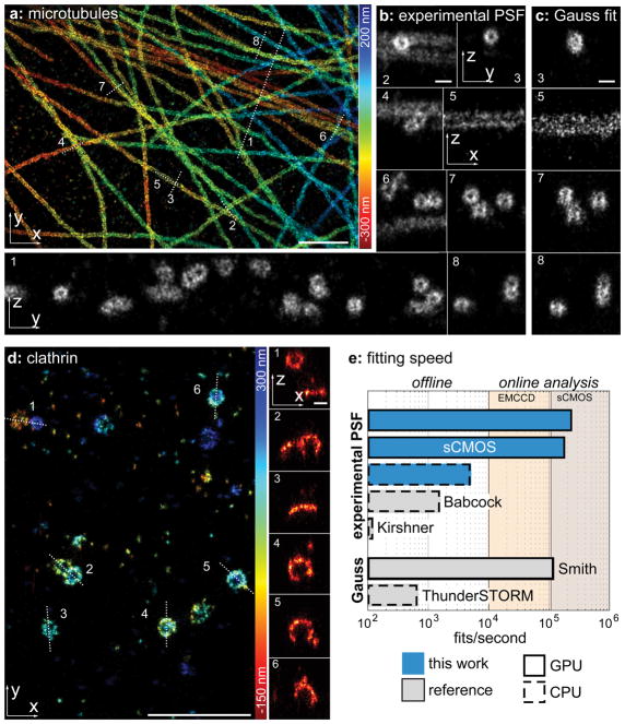
Figure 1
(a) Immunolabeled microtubules imaged using the DNA-PAINT 15 approach. Localizations are color-coded according to their z-position. Corresponding localization precisions and profiles are shown in Supp...
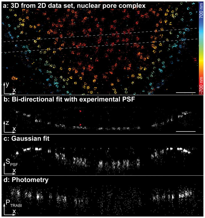
Figure 2
Our spline fitter extracts accurate 3D positions from a simple 2D dataset with an unmodified PSF
(a) Nup107-SNAP-AlexaFluor647 was imaged using dSTORM on a standard microscope without 3D optics. ( b ) Side-view reconstruction of the region denoted in (a). The nucleoplasmic and cytoplasmic rings o...
Figure images are served from the NIH/NLM PubMed Central Open Access Subset or Europe PMC; copyright remains with the publishers and authors.
💬 Discussion
0 commentsNo comments yet. Be the first to start a discussion!
Leave a Comment