Abstract
Visual neuroscientists require accurate control of visual stimulation. However, few stimulator solutions simultaneously offer high spatio-temporal resolution and free control over the spectra of the light sources, because they rely on off-the-shelf technology developed for human trichromatic vision. Importantly, consumer displays fail to drive UV-shifted short wavelength-sensitive photoreceptors, which strongly contribute to visual behaviour in many animals, including mice, zebrafish and fruit flies. Moreover, many non-mammalian species feature more than three spectral photoreceptor types. Here, we present a flexible, spatial visual stimulator with up to six arbitrary spectrum chromatic channels. It combines a standard digital light processing engine with open source hard- and software that can be easily adapted to the experimentalist's needs. We demonstrate the capability of this general visual stimulator experimentally in the in vitro mouse retinal whole-mount and the in vivo zebrafish. With this work, we intend to start a community effort of sharing and developing a common stimulator design for vision research.
🔬 Techniques
🔭 Microscopes
🧬 Organisms
💻 Software
✨ Fluorophores
🧪 Sample Preparation
🏭 Microscope Brands
🧪 Reagent Suppliers
🔴 Lasers
📷 Detectors
🔎 Objectives
🎨 Filters
💻 Software Details
💻 Code & Software
QDSpy - a Python software for scripting and presenting stimuli for visual neuroscience.
QDSpy - a Python software for scripting and presenting stimuli for visual neuroscience.
An arbitrary-spectrum spatial visual stimulator for vision research
An arbitrary-spectrum spatial visual stimulator for vision research
💾 Data Repositories
🏛️ Research Organizations (ROR)
Affiliated research institutions:
📋 Methods
Key resources table
Reagent type (species) or resource Designation Source or reference Identifiers Additional information Genetic reagent ( Mus musculus ) HR2.1:TN-XL Wei et al., 2012 Dr. Bernd Wissinger (Tübingen University) Genetic reagent ( Danio rerio ) tg(1.8ctbp2:SyGCaMP6f) Rosa et al., 2016 Dr. Leon Lagnado (Sussex University) Software, algorithm KiCad EDA http://kicad-pcb.org/ Electronics design software Software, algorithm OpenSCAD http://www.openscad.org 3D CAD software Note that the general stimulator design, operation and performance testing is described in the Results section. The respective parts for the mouse and the zebrafish stimulator versions are listed in Tables 2 and 3 , respectively. Hence, this section focuses on details about the calibration procedures, 2P imaging, animal procedures, and data analysis.
Intensity calibration and gamma correction
The purpose of the intensity calibration is to ensure that each LED evokes a similarly maximal photoisomerisation rate in its respective spectral cone type, whereas the gamma correction aims at linearising each LED’s intensity curve. All calibration procedures are described in detail in the iPython notebooks included in the open-visual-stimulator GitHub repository (for link, see Table 1 ). In case of the mouse stimulator , we used a photo-spectrometer (USB2000, 350–1000 nm, Ocean Optics, Ostfildern, Germany) that can be controlled and read-out from the iPython notebooks. It was coupled by an optic fibre and a cosine corrector (FOV 180°, 3.9 mm aperture) to the bottom of the recording chamber of the 2P microscope and positioned approximately in the stimulator’s focal plane. For intensity calibration, we displayed a bright spot (1,000 µm in diameter, max. intensity) of green and UV light to obtain spectra of the respective LEDs. We used a long integration time (1 s) and fitted the average of several reads (n = 10 for green; n = 50 reads for UV) with a Gaussian to remove shot noise. This yielded reliable measurements also at low LED intensities, which was particularly critical for UV LEDs. The spectrometer output ( S m e a s ) was divided by the integration time ( Δ t , in s) to obtain counts/s and then converted into electrical power ( P e l , in nW) using the calibration data ( S C a l , in µJ/count) provided by Ocean Optics, (1) P e l ( λ ) = S M e a s ( λ ) / Δ t ⋅ S C a l ( λ ) ⋅ 10 3 , with wavelength λ . To obtain the photoisomerisation rate per photoreceptor type, we first converted from electrical power into energy flux ( P e f l u x , in eV/s), (2) P e f l u x ( λ ) = P e l ( λ ) ⋅ a ⋅ 10 − 9 , where a = 6.242 ⋅10 18 eV/J. Next, we calculated the photon flux ( P P h i , in photons/s) using the photon energy Q ( P Q , in eV), (3) P Q ( λ ) = c ⋅ h / ( λ ⋅ 10 − 9 ) , (4) P P h i ( λ ) = P e f l u x ( λ ) / P Q ( λ ) , with the speed of light, c = 299,792,458 m/s, and Planck’s constant, h = 4.135667 ⋅10 -15 eV⋅s. The photon flux density ( P E , [photons/s/µm 2 ]) was then computed as (5) P E ( λ ) = P P h i ( λ ) / A S t i m , where A S t i m (in µm 2 ) corresponds to the light stimulus area. To convert P E into photoisomerisation rate, we next determined the effective activation ( S A c t ) of mouse photoreceptor types by the LEDs as (6) S A c t ( λ ) = S O p s i n ( λ ) ⋅ S L E D ( λ ) with the peak-normalised spectra of the M- and S-opsins, S O p s i n , and the green and UV LEDs, S L E D . Sensitivity spectra of mouse opsins were derived from Equation 8 in Stockman and Sharpe (2000) . For our LEDs ( Table 2 ), the effective mouse M-opsin activation was 14.9% and 10.5% for the green and UV LED, respectively. The mouse S-opsin is only expected to be activated by the UV LED (52.9%) ( Figure 3a, f ). Next, we estimated the photon flux ( R P h , [photons/s]) for each photoreceptor as (7) R P h ( λ ) = P E ( λ ) ⋅ A C o l l e c t where A C o l l e c t = 0.2 µm 2 corresponds to the light collection area of cone outer segments ( Nikonov et al., 2006 ). The photoisomerisation rate ( R I s o , P*/photoreceptor/s) for each combination of LED and photoreceptor type was estimated using (8) R I s o = ∑ R P h ( λ ) ⋅ S A c t ( λ ) , see Nikonov et al. (2006) for details. The intensities of the mouse stimulator LEDs were manually adjusted ( Figure 2—figure supplement 5b,c ) to an approximately equal photoisomerisation range from (in P*/cone/s ⋅10 3 ) 0.6 and 0.7 (stimulator shows black image) to 19.5 and 19.2 (stimulator shows white image) for M- and S-opsins, respectively ( cf . Figure 3f ). This corresponds to the low photopic range. The M-opsin sensitivity spectrum displays a ‘tail’ in the short wavelength range (due to the opsin’s β-band, see Figure 1a and Stockman and Sharpe, 2000 ), which means that it should be cross-activated by our UV LED. Specifically, while S-opsin should be solely activated by the UV LED (19.2 by UV vs. 0.1 by green; in P*/cone/s ⋅10 3 ), we expect M-opsin to be activated by both LEDs (19.5 by green vs. 3.8 by UV). The effect of such cross-activation can be addressed, for instance, by silent substitution (see below). To account for the non-linearity of the stimulator output using gamma correction, we recorded spectra for each LED for different intensities (1,000 µm spot diameter; pixel values from 0 to 254 in steps of 2) and estimated the photoisomerisation rates, as described above. From these data, we computed a lookup table (LUT) that allows the visual stimulus software (QDSpy) to linearise the intensity functions of each LED ( cf . Figure 3e ; for details, see iPython notebooks; Table 1 ). In case of the zebrafish stimulator , to determine the LED spectra, we used a compact CCD Spectrometer (CCS200/M, Thorlabs, Dachau, Germany) in combination with the Thorlabs Optical Spectrum Analyzers (OSA) software, coupled to a linear fibre patch cable. To determine the electrical power ( P e l , in nW), we used an optical energy power meter (PM100D, Thorlabs) in combination with the Thorlabs Optical Power Monitor (OPM) software, coupled to a photodiode power sensor (S130VC, Thorlabs). Both probes were positioned behind the teflon screen (0.15 mm, for details, see Table 3 ). Following the same procedure as described above, we determined the photoisomerisation rate ( R I s o , P*/photoreceptor/s) for each combination of LED and photoreceptor type ( cf. iPython notebooks; Table 1 ).
Show full methods section
Key resources table
Reagent type (species) or resource Designation Source or reference Identifiers Additional information Genetic reagent ( Mus musculus ) HR2.1:TN-XL Wei et al., 2012 Dr. Bernd Wissinger (Tübingen University) Genetic reagent ( Danio rerio ) tg(1.8ctbp2:SyGCaMP6f) Rosa et al., 2016 Dr. Leon Lagnado (Sussex University) Software, algorithm KiCad EDA http://kicad-pcb.org/ Electronics design software Software, algorithm OpenSCAD http://www.openscad.org 3D CAD software Note that the general stimulator design, operation and performance testing is described in the Results section. The respective parts for the mouse and the zebrafish stimulator versions are listed in Tables 2 and 3 , respectively. Hence, this section focuses on details about the calibration procedures, 2P imaging, animal procedures, and data analysis.
Intensity calibration and gamma correction
The purpose of the intensity calibration is to ensure that each LED evokes a similarly maximal photoisomerisation rate in its respective spectral cone type, whereas the gamma correction aims at linearising each LED’s intensity curve. All calibration procedures are described in detail in the iPython notebooks included in the open-visual-stimulator GitHub repository (for link, see Table 1 ). In case of the mouse stimulator , we used a photo-spectrometer (USB2000, 350–1000 nm, Ocean Optics, Ostfildern, Germany) that can be controlled and read-out from the iPython notebooks. It was coupled by an optic fibre and a cosine corrector (FOV 180°, 3.9 mm aperture) to the bottom of the recording chamber of the 2P microscope and positioned approximately in the stimulator’s focal plane. For intensity calibration, we displayed a bright spot (1,000 µm in diameter, max. intensity) of green and UV light to obtain spectra of the respective LEDs. We used a long integration time (1 s) and fitted the average of several reads (n = 10 for green; n = 50 reads for UV) with a Gaussian to remove shot noise. This yielded reliable measurements also at low LED intensities, which was particularly critical for UV LEDs. The spectrometer output ( S m e a s ) was divided by the integration time ( Δ t , in s) to obtain counts/s and then converted into electrical power ( P e l , in nW) using the calibration data ( S C a l , in µJ/count) provided by Ocean Optics, (1) P e l ( λ ) = S M e a s ( λ ) / Δ t ⋅ S C a l ( λ ) ⋅ 10 3 , with wavelength λ . To obtain the photoisomerisation rate per photoreceptor type, we first converted from electrical power into energy flux ( P e f l u x , in eV/s), (2) P e f l u x ( λ ) = P e l ( λ ) ⋅ a ⋅ 10 − 9 , where a = 6.242 ⋅10 18 eV/J. Next, we calculated the photon flux ( P P h i , in photons/s) using the photon energy Q ( P Q , in eV), (3) P Q ( λ ) = c ⋅ h / ( λ ⋅ 10 − 9 ) , (4) P P h i ( λ ) = P e f l u x ( λ ) / P Q ( λ ) , with the speed of light, c = 299,792,458 m/s, and Planck’s constant, h = 4.135667 ⋅10 -15 eV⋅s. The photon flux density ( P E , [photons/s/µm 2 ]) was then computed as (5) P E ( λ ) = P P h i ( λ ) / A S t i m , where A S t i m (in µm 2 ) corresponds to the light stimulus area. To convert P E into photoisomerisation rate, we next determined the effective activation ( S A c t ) of mouse photoreceptor types by the LEDs as (6) S A c t ( λ ) = S O p s i n ( λ ) ⋅ S L E D ( λ ) with the peak-normalised spectra of the M- and S-opsins, S O p s i n , and the green and UV LEDs, S L E D . Sensitivity spectra of mouse opsins were derived from Equation 8 in Stockman and Sharpe (2000) . For our LEDs ( Table 2 ), the effective mouse M-opsin activation was 14.9% and 10.5% for the green and UV LED, respectively. The mouse S-opsin is only expected to be activated by the UV LED (52.9%) ( Figure 3a, f ). Next, we estimated the photon flux ( R P h , [photons/s]) for each photoreceptor as (7) R P h ( λ ) = P E ( λ ) ⋅ A C o l l e c t where A C o l l e c t = 0.2 µm 2 corresponds to the light collection area of cone outer segments ( Nikonov et al., 2006 ). The photoisomerisation rate ( R I s o , P*/photoreceptor/s) for each combination of LED and photoreceptor type was estimated using (8) R I s o = ∑ R P h ( λ ) ⋅ S A c t ( λ ) , see Nikonov et al. (2006) for details. The intensities of the mouse stimulator LEDs were manually adjusted ( Figure 2—figure supplement 5b,c ) to an approximately equal photoisomerisation range from (in P*/cone/s ⋅10 3 ) 0.6 and 0.7 (stimulator shows black image) to 19.5 and 19.2 (stimulator shows white image) for M- and S-opsins, respectively ( cf . Figure 3f ). This corresponds to the low photopic range. The M-opsin sensitivity spectrum displays a ‘tail’ in the short wavelength range (due to the opsin’s β-band, see Figure 1a and Stockman and Sharpe, 2000 ), which means that it should be cross-activated by our UV LED. Specifically, while S-opsin should be solely activated by the UV LED (19.2 by UV vs. 0.1 by green; in P*/cone/s ⋅10 3 ), we expect M-opsin to be activated by both LEDs (19.5 by green vs. 3.8 by UV). The effect of such cross-activation can be addressed, for instance, by silent substitution (see below). To account for the non-linearity of the stimulator output using gamma correction, we recorded spectra for each LED for different intensities (1,000 µm spot diameter; pixel values from 0 to 254 in steps of 2) and estimated the photoisomerisation rates, as described above. From these data, we computed a lookup table (LUT) that allows the visual stimulus software (QDSpy) to linearise the intensity functions of each LED ( cf . Figure 3e ; for details, see iPython notebooks; Table 1 ). In case of the zebrafish stimulator , to determine the LED spectra, we used a compact CCD Spectrometer (CCS200/M, Thorlabs, Dachau, Germany) in combination with the Thorlabs Optical Spectrum Analyzers (OSA) software, coupled to a linear fibre patch cable. To determine the electrical power ( P e l , in nW), we used an optical energy power meter (PM100D, Thorlabs) in combination with the Thorlabs Optical Power Monitor (OPM) software, coupled to a photodiode power sensor (S130VC, Thorlabs). Both probes were positioned behind the teflon screen (0.15 mm, for details, see Table 3 ). Following the same procedure as described above, we determined the photoisomerisation rate ( R I s o , P*/photoreceptor/s) for each combination of LED and photoreceptor type ( cf. iPython notebooks; Table 1 ).
Spatial resolution measurements
To measure the spatial resolution of the mouse stimulator, we removed the lens of a Raspberry Pi camera chip (OV5647, Eckstein GmbH, Clausthal-Zellerfeld, Germany) and positioned it at the level of the recording chamber. Then, we projected UV and green checkerboards of varying checker sizes (2, 3, 4, 5, 10, 20, 30, 40, 60, 80, and 100 µm) through an objective lens (MPL5XBD (5x), Olympus, Germany) or through the condenser onto the chip of the camera ( Figure 4a ). For each checker size and LED, we extracted intensity profiles using ImageJ ( Figure 4b ) and estimated the respective contrast as I M a x - I M i n ( Figure 4c ). To quantify the steepness of the transition between bright and dark checkers, we peak-normalised the intensity profiles and normalised relative to half-width of the maximum ( Figure 4d ). Next, we fitted a sigmoid to the rising phase of the intensity profile (9) y = K 0 + K 1 / ( 1 + e x p ( - ( x - K 2 ) / K 3 ) ) and used 1 / K 3 as estimate of the rise time and as a proxy for ‘sharpness’ of the transitions between black and white pixels ( Figure 4e ). To measure the difference in focal plane of UV and green LED due to chromatic aberration, we projected a 40 and 100 µm checkerboard through a 20x objective (W Plan-Apochromat 20×/1.0 DIC M27, Zeiss, Oberkochen, Germany) onto the Raspberry Pi camera (see above).
Fast intensity measurements
To verify temporal separation, we measured the time course of the green LED (mouse stimulator) with and without blanking using a PMT positioned at the level of the recording chamber ( Figure 2—figure supplement 2a ). Traces were recorded with pClamp at 250 kHz (Molecular Devices, Biberach an der Riss, Germany). To estimate the amount of intensity modulation due to aliasing ( Figure 2—figure supplement 2b ), we measured the intensity of both LEDs together (‘white’) driven by a chirp stimulus with blanking at the same position using a photodiode (Siemens silicon photodiode BPW 21, Reichelt, Sande, Germany; as light-dependent current source in a transimpedance amplifier circuit). Next, intensity traces were box-smoothed with a box width of 100 ms, which roughly corresponds to the integration time of mouse cone photoreceptors ( Umino et al., 2008 ). Silent substitution For our measurements in mouse cones, we used a silent substitution protocol ( Estévez and Spekreijse, 1982 ) for generating opsin-isolating stimuli to account for the cross-activation of mouse M-opsin by the UV LED. Here, one opsin type is selectively stimulated by presenting a scaled, counterphase version of the stimulus to all other opsin types ( cf . Figure 5 ). Specifically, we first used the ratio of activation (as photoisomerisation rate) of M-opsin by UV and green to estimate the amount of cross-activation ( S C r o s s A c t ). For our recordings, an activation of M-opsin of 19.5 and 3.8 P*/cone/s ⋅10 3 for green and UV LED resulted in a cross-activation of S C r o s s A c t = 0.195. Then, S C r o s s A c t was used to scale the intensity of the counterphase stimulus: (10) I G = I - I U V ⋅ S C r o s s A c t For our recordings in zebrafish larvae, we did not use silent substitution. However, we describe a possible approach for the zebrafish (or a comparable tetrachromatic species) in our online resources ( Table 1 ).
Animals and tissue preparation
All animal procedures (mice) were approved by the governmental review board (Regierungspräsidium Tübingen, Baden-Württemberg, Konrad-Adenauer-Str. 20, 72072 Tübingen, Germany) and performed according to the laws governing animal experimentation issued by the German Government. All animal procedures (zebrafish) were performed in accordance with the UK Animals (Scientific Procedures) Act 1986 and approved by the animal welfare committee of the University of Sussex (zebrafish larvae). For the mouse experiments, we used one 12-week-old HR2.1:TN-XL mouse; this mouse line expresses the ratiometric Ca 2+ biosensor TN-XL under the cone-specific HR2.1 promoter and allows measuring light-evoked Ca 2+ responses in cone synaptic terminals ( Wei et al., 2012 ). Animals were housed under a standard 12 hr day-night rhythm. Before the recordings, the mouse was dark-adapted for ≥1 hr, then anaesthetized with isoflurane (Baxter, Unterschleißheim, Germany) and killed by cervical dislocation. The eyes were removed and hemisected in carboxygenated (95% O 2 , 5% CO 2 ) artificial cerebrospinal fluid (ACSF) solution containing (in mM): 125 NaCl, 2.5 KCl, 2 CaCl 2 , 1 MgCl 2 , 1.25 NaH 2 PO 4 , 26 NaHCO 3 , 20 glucose, and 0.5 L-glutamine (pH 7.4). The retina was separated from the eye-cup, cut in half, flattened, and mounted photoreceptor side-up on a nitrocellulose membrane (0.8 mm pore size, Merck Millipore, Darmstadt, Germany). Using a custom-made slicer ( Wei et al., 2012 ; Werblin, 1978 ), acute vertical slices (200 µm thick) were cut parallel to the naso-temporal axis. Slices attached to filter paper were transferred on individual glass coverslips, fixed using high-vacuum grease and kept in a storing chamber at room temperature for later use. For imaging, individual retinal slices were transferred to the recording chamber of the 2P microscope (see below), where they were continuously perfused with warmed (36°C), carboxygenated extracellular solution. For the zebrafish larvae experiments, we used 7 day post fertilisation ( dpf) larvae of the zebrafish ( Danio rerio) line tg(1.8ctbp2:SyGCaMP6f) , which expresses the genetically encoded Ca 2+ indicator GCaMP6f fused with synaptophysin under the RibeyeA promoter and allows measuring light-evoked Ca 2+ responses in bipolar cell synaptic terminals ( Dreosti et al., 2009 ; Johnston et al., 2019 ; Rosa et al., 2016 ; Zimmermann et al., 2018 ). Animals were grown from 10 hr post fertilisation ( hpf) in 200 µM of 1-phenyl-2-thiourea (Sigma) to prevent melanogenesis ( Karlsson et al., 2001 ). Animals were housed under a standard 14/10 hr day-night rhythm and fed 3x a day. Before the recordings, zebrafish larvae were immobilised in 2% low-melting-point agarose (Fischer Scientific, Loughborough, UK; Cat: BP1360-100), placed on a glass coverslip and submersed in fish water. To prevent eye movement during recordings, α-bungarotoxin (1 nl of 2 mg/ml; Tocris, Bristol, UK; Cat: 2133) was injected into the ocular muscles behind the eye.
Two-photon imaging
For all imaging experiments, we used MOM-type two-photon (2P) microscopes (designed by W. Denk, MPI, Heidelberg; purchased from Sutter Instruments/Science Products, Hofheim, Germany). For image acquisition, we used custom software (ScanM by M. Müller, MPI Neurobiology, Munich, and T.E.) running under IGOR Pro 6.3 for Windows (Wavemetrics, Lake Oswego, OR). The microscopes were equipped each with a mode-locked Ti:Sapphire laser (MaiTai-HP DeepSee, Newport Spectra-Physics, Darmstadt, Germany; or Chameleon Vision-S, Coherent; Ely, UK), two fluorescence detection channels for eCFP (FRET donor; HQ 483/32, AHF, Tübingen, Germany) and citrine (FRET acceptor; HQ 538/50, AHF) or GCaMP6f (ET 525/70 or ET 525/50, AHF), and a water immersion objective (W Plan-Apochromat 20×/1.0 DIC M27, Zeiss, Oberkochen, Germany). The excitation laser was tuned to 860 nm and 927 nm for TN-XL (eCFP) in mouse and GCaMP6f in zebrafish, respectively. Time-lapsed image series were recorded with 64 × 16 pixels (at 31.25 Hz) or 128 × 64 (at 15.625 Hz). Detailed descriptions of the setups for mouse ( Euler et al., 2019 ; Euler et al., 2009 ; Franke et al., 2017 ) and zebrafish ( Zimmermann et al., 2018 ) have been published elsewhere.
Data analysis
Data analysis was performed using IGOR Pro (Wavemetrics). Regions of interest (ROIs) of individual synaptic terminals (of mouse cones and zebrafish bipolar cells) were manually placed. Then, Ca 2+ traces for each ROI were extracted for mouse cones as Δ R / R , with the ratio R = F A / F D of the FRET acceptor (citrine) and donor (eCFP) fluorescence, and resampled at 500 Hz. For zebrafish bipolar cells, Ca 2+ traces for each ROI were extracted and detrended by high-pass filtering above ~0.1 Hz, followed by z-normalisation based on the time interval 1–6 s at the beginning of recordings using custom-written routines under IGOR Pro. A stimulus synchronisation marker that was generated by the visual stimulation software (Results) and embedded in the recordings served to align the Ca 2+ traces relative to the stimulus with ≤2 ms precision (depending on the scan line duration, see Results and Euler et al., 2019 ). For this, the timing for each ROI was corrected for sub-frame time-offsets related to the scanning. Response quality index . To measure how well a cell responded to the sine wave stimulus, we computed the signal-to-noise ratio (11) Q i = V a r [ ( C ) r ] t ( V a r [ C ] t ) r where C is the T by R response matrix (time samples by stimulus repetitions), while ( ) x and V a r [ ] x denote the mean and variance across the indicated dimension, respectively ( Baden et al., 2016 ; Franke et al., 2017 ). For further analysis, we used only cells that had a Q i > 0.3 . Spectral contrast . The mean trace in response to the green and UV sine wave stimulus was used to analyse the spectral sensitivity of the cones. For that, we computed the power spectrum of the trace and used the power ( P ) at the fundamental frequency (1 Hz) as a measure of response strength. Then, the spectral contrast ( S C ) was estimated as (12) S C = P G − P B P G + P B , where P G and P B correspond to the responses to green and UV, respectively. For statistical comparison of S C values with and without silent substitution (see above), we used the Wilcoxon signed-rank test for non-parametric, paired samples.
Additional files 10.7554/eLife.48779.019 Supplementary file 1. Parts list of the through-the-objective mouse stimulator ( cf . Figure 2—figure supplement 1 ; entries in grey are not shown). 10.7554/eLife.48779.020 Transparent reporting form
📊 Figures
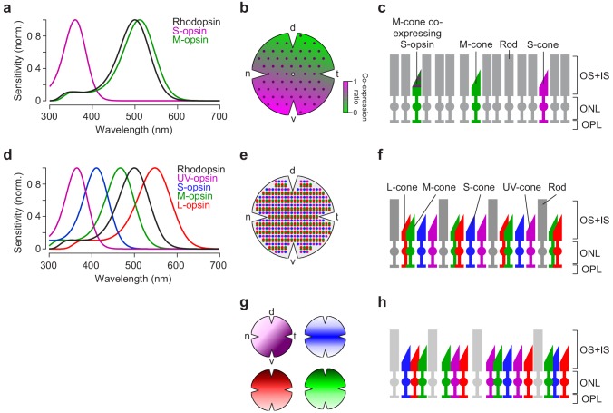
Figure 1.
Photoreceptor types and distribution in mouse and zebrafish retina.
( a ) Peak-normalised sensitivity profiles of mouse S- (magenta) and M-opsin (green) as well as rhodopsin (black; profiles were estimated following Stockman and Sharpe, 2000 ). ( b ) Schematic drawing...
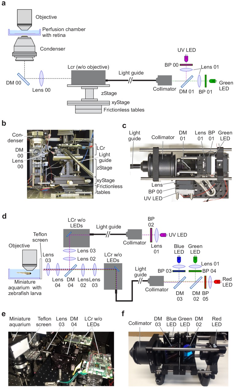
Figure 2.
Visual stimulator design.
( a ) Schematic drawing of the dichromatic stimulator for in vitro recordings of mouse retinal explants. The stimulator is coupled into the two-photon (2P) microscope from below the recording chamber ...
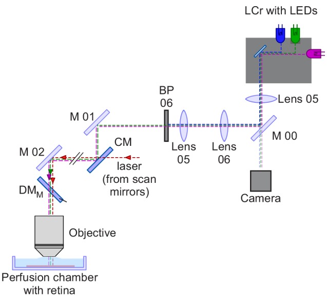
Figure 2u2014figure supplement 1.
Optical pathway for a through-the-objective (TTO) mouse stimulator.
Schematic drawing of a TTO dichromatic stimulator for in vitro recordings of mouse retinal explants ( cf . Euler et al., 2009 ). The light from the LCr with internal UV, blue and green LEDs is filtere...
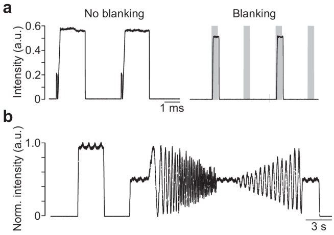
Figure 2u2014figure supplement 2.
Intensity measurements of the LEDs of the mouse stimulator.
( a ) Intensity of green LED measured with a PMT (at 250 kHz; for details, see Materialsu00a0andu00a0methods) without (left) and with blanking (right); grey shading indicates blanking signal. ( b ) Sm...
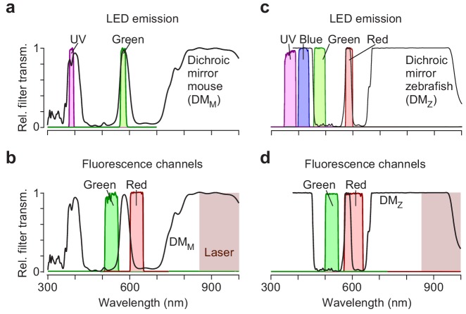
Figure 2u2014figure supplement 3.
Spectral separation of visual stimulation and fluorescence detection.
( a ) Relative transmission of filters in front of UV and green LED as well as of dichroic mirror on top of objective ( cf . Euler et al., 2009 ). ( b ) Same as ( a ), for filters in front of PMTs (Ma...
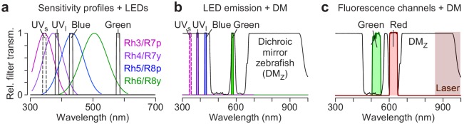
Figure 2u2014figure supplement 4.
Suggestion for LED/filter design for a Drosophila visual stimulator.
( a ) Spectral sensitivity of rhodopsins expressed in the four types of inner photoreceptors (Rh3: short-UV; Rh4: long-UV; Rh5: blue; Rh6: green) of Drosophila (data from Schnaitmann et al., 2018 , ba...
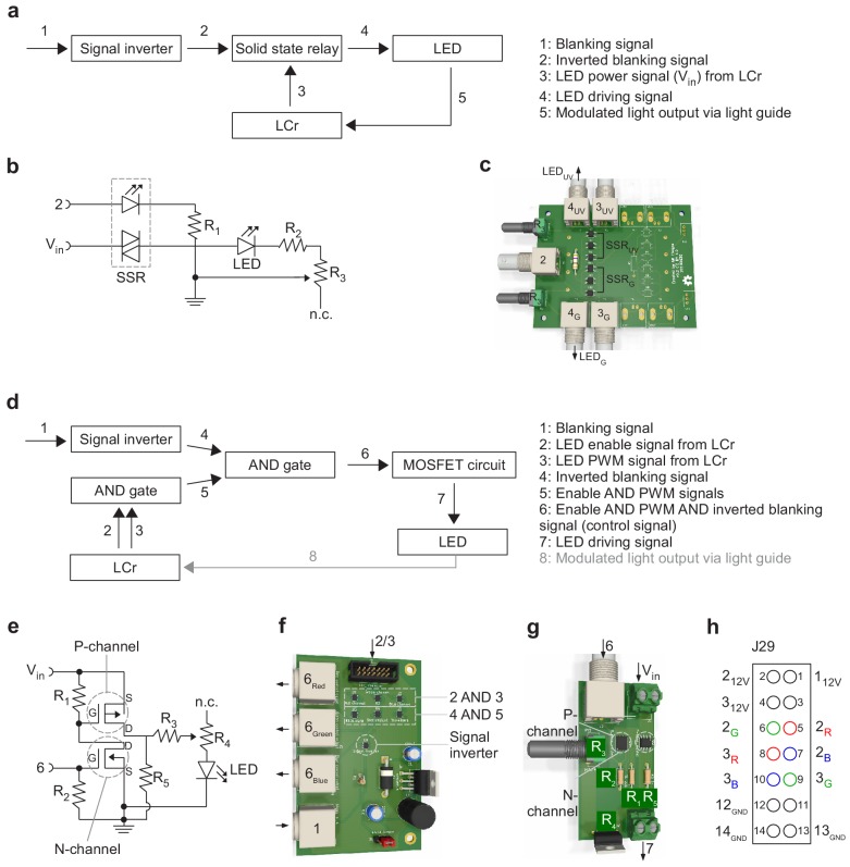
Figure 2u2014figure supplement 5.
External LED control and temporal separation of stimulation and fluorescence detection.
( a ) Schematic illustrating the circuit that ensures that the stimulator LEDs are only on during the microscope's scanner retrace (for details, see Results). The u2018laser blankingu2019 signal (1) g...
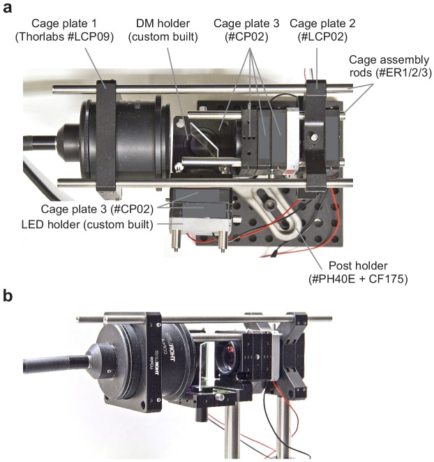
Figure 2u2014figure supplement 6.
Detailed description of external LED unit of the mouse stimulator.
( a ) Top-view of external LED illumination unit, with ordering numbers of all parts purchased from Thorlabs indicated (see also Table 2 ). Cage plates #LCP02 holds filters and lenses with a diameter ...
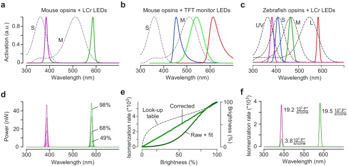
Figure 3.
Calibration of the mouse stimulator.
( a ) Sensitivity profiles of mouse S- and M-opsin (dotted black lines) and spectra of UV (magenta) and green LED/filter combinations used in the mouse stimulator. ( b ) Sensitivity profiles of mouse ...
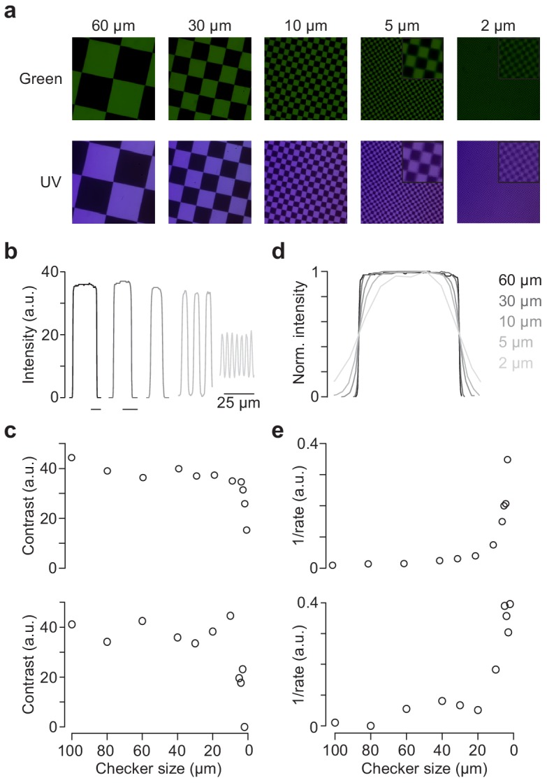
Figure 4.
Spatial calibration of the mouse stimulator.
( a ) Images of checkerboard stimuli with varying checker sizes projected through-the-objective (TTO) for illumination with green (top) and UV (bottom) LED, recorded by placing the sensor chip of a Ra...
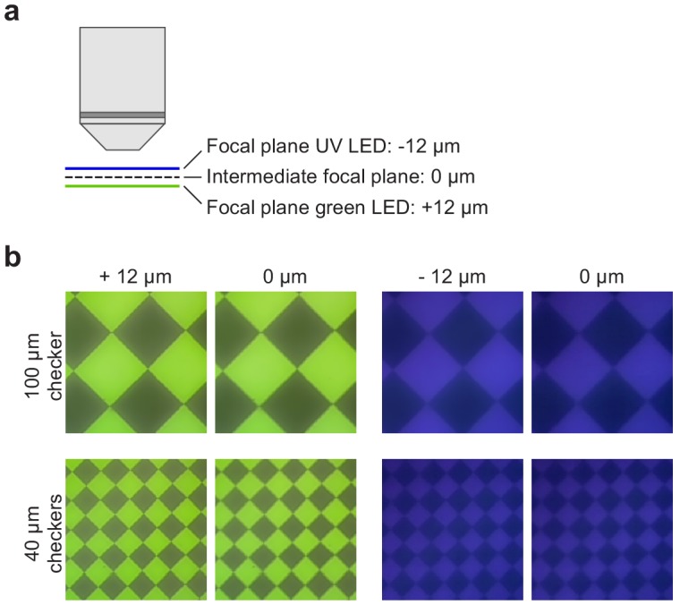
Figure 4u2014figure supplement 1.
Chromatic aberration of the mouse stimulator.
( a ) Schematic illustrating the chromatic aberration-related difference in focal planes of UV and green image in the TTO configuration. ( b ) Images of a 100 (top) and 40 (bottom) u00b5m checkerboard...
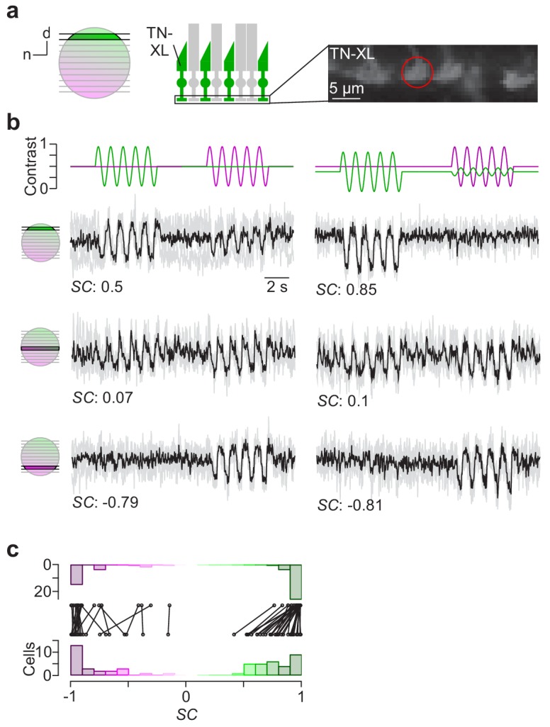
Figure 5.
Cone-isolating stimulation of mouse cones.
( a ) Dorsal recording field in the outer plexiform layer (OPL; right) shows labelling of cone axon terminals with Ca 2+ biosensor TN-XL in the HR2.1:TN-XL mouse line ( Wei et al., 2012 ). Schematic o...
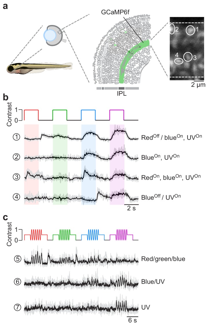
Figure 6.
Chromatic responses in bipolar cells of in vivo zebrafish larvae.
( a ) Drawing illustrating the expression of the genetically encoded Ca 2+ biosensor SyGCaMP6f in bipolar cell terminals (left) of tg(1.8ctbp2:SyGCaMP6f) zebrafish larvae and scan field of inner plexi...
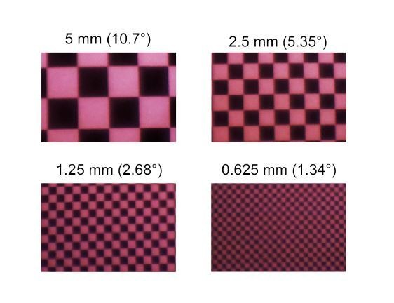
Author response image 1.
Images of checkerboard stimuli with varying sizes for UV LED of the zebrafish stimulator, recorded using a Raspberry Pi camera positioned between the LCrs and the teflon screen.
Figure images are served from the NIH/NLM PubMed Central Open Access Subset or Europe PMC; copyright remains with the publishers and authors.
💬 Discussion
0 commentsNo comments yet. Be the first to start a discussion!
Leave a Comment