Abstract
Abstract Tomographic reconstruction of cryopreserved specimens imaged in an electron microscope followed by extraction and averaging of sub-volumes has been successfully used to derive atomic models of macromolecules in their biological environment. Eliminating biochemical isolation steps required by other techniques, this method opens up the cell to in-situ structural studies. However, the need to compensate for errors in targeting introduced during mechanical navigation of the specimen significantly slows down tomographic data collection thus limiting its practical value. Here, we introduce protocols for tilt-series acquisition and processing that accelerate data collection speed by up to an order of magnitude and improve map resolution compared to existing approaches. We achieve this by using beam-image shift to multiply the number of areas imaged at each stage position, by integrating geometrical constraints during imaging to achieve high precision targeting, and by performing per-tilt astigmatic CTF estimation and data-driven exposure weighting to improve final map resolution. We validated our beam image-shift electron cryo-tomography (BISECT) approach by determining the structure of a low molecular weight target (~300 kDa) at 3.6 Å resolution where density for individual side chains is clearly resolved.
🔬 Techniques
🔭 Microscopes
🧬 Organisms
💻 Software
✨ Fluorophores
🧪 Sample Preparation
🏭 Microscope Brands
🧪 Reagent Suppliers
📷 Detectors
💻 Software Details
💻 Code & Software
💾 Data Repositories
🏛️ Research Organizations (ROR)
Affiliated research institutions:
📋 Methods
Sample preparation dNTPase was cloned into pMCSG7 using LIC cloning, Supplementary Table 3 . It was then transformed in BL21(DE3) and grown in Terrific Broth (TB) medium with 4% glycerol, ampicillin (100 µg/ml). Cultures were induced with IPTG (final concentration 0.2 mM), and grown for an additional 14–18 h at 20 °C before harvesting by centrifugation. Cell pellets were resuspended in approximately 5 mL Buffer A (100 mM Tris pH 7.9, 500 mM NaCl, 30 mM imidazole, 5% glycerol) per 1 g of cell paste. All purification steps were performed at 4 °C. Resuspended cells were incubated with DNase (4 mg), lysozyme (40 mg), and MgCl 2 (2 mM). Cells were lysed by three 1 min sonication cycles at 60% power using a Branson 450 Digital Sonifier with at least 2 min between cycles and clarified by centrifugation at 30,000 g for 30 min. The soluble fractions were loaded onto a 5-mL HisTrap Ni-NTA column (GE Healthcare) in Buffer A and eluted with an imidazole gradient from 45 to 300 mM. Sample was dialyzed overnight into Buffer B (50 mM Tris pH 7.9, 100 mM NaCl, 5% glycerol) at 4 °C and treated with tobacco etch virus (TEV) protease (1:30 ratio TEV:dNTPase plus 2 mM DTT) to remove the purification (polyhistidine) tag, and then applied to a 5-mL HisTrap Ni NTA column. The flow-through fraction was further purified by size exclusion chromatography with a HiLoad 16/600 Superdex 200 column (GE Healthcare) in Buffer C (50 mM Tris pH 7.9, 100 mM NaCl, 10% glycerol). Peak fractions were pooled, concentrated to 10–20 mg/mL, aliquoted, flash cooled with liquid N 2 , and stored at −80 °C. Grid preparation 1–1.5 mg protein was thawed then run over a 10/30 Superdex 200 Increase column (GE Healthcare) in Buffer D (20 mM Tris pH 7.5, 100 mM NaCl). 2 parts of the peak fraction at about 1.3 mg/mL was mixed of with 1 part of 6 nm gold fiducials that were 20x concentrated and buffer exchanged in Buffer D. 3uL of the mix was applied on a UltrAuFoil R1.2/1.3 300 mesh grid (Quantifoil Micro Tools GmbH). Grids were previously glow-discharged for 30 sec at 15 mA (PELCO easiGlow™, Ted Pella, Inc.). The excess sample was removed by blotting for 3 s using filter paper (Whatman #1) and grids were plunged-frozen in liquid ethane (−182 °C) using a vitrification robot (EM GP2, Leica Microsystems). dNTPase data collection Data were collected at 300 keV under parallel beam illumination on a Titan Krios (Thermo Fisher Scientific) housed at the NCI cryoEM facility affiliated with the NIH IRP CryoEM Consortium (NICE). Images were recorded on a direct electron detector (K2 summit, Gatan Inc.) placed behind an energy filter (Bioquantum, Gatan Inc.) operated with a 20 eV slit. Tilt-series were collected using SerialEM (version 3.8beta8) 15 . An initial set of 125 tilt-series were collected using a ±60° range grouped dose-symmetric scheme (0, 3, −3, −6, 6, 9, −9, −12, 12, 15, −15, −18, −21, 18, 21, 24, 27, −24, −27, −30, −33, 30, 33, 36, 39, 42, −36, −39, −42, −45, −48, 45, 48, 51, 54, 57, 60, −51, −54, −57, −60) with a dose of ~3e − /Å 2 per tilt angle (4 frames per movie, ~120 e − /Å 2 total dose). An additional 275 tilt-series were collected using a similar tilt scheme as before but with a ± 36° range (0, 3, −3, −6, 6, 9, −9, −12, 12, 15, −15, −18, −21, 18, 21, 24, −24, −27, −30, 27, 30, 33, 36, −33, −36) and a dose of ~5e − /Å 2 per tilt angle (11 frames per movie, ~120 e − /Å 2 total dose). Additional CET data collection statistics are included in Supplementary Table 1 . The SPA dataset was collected using a total dose of ~60 e − /Å 2 . For all three datasets, each area was collected with a pixel size of 1.37 Å/pix using a 5 × 5-hole lattice with the stage centered on the target area and each hole acquired using BIS. The two CET datasets were used for structure determination by SVA and CSPT and the single-particle dataset was subjected to SPA refinement, Supplementary Table 2 .
Show full methods section
Sample preparation dNTPase was cloned into pMCSG7 using LIC cloning, Supplementary Table 3 . It was then transformed in BL21(DE3) and grown in Terrific Broth (TB) medium with 4% glycerol, ampicillin (100 µg/ml). Cultures were induced with IPTG (final concentration 0.2 mM), and grown for an additional 14–18 h at 20 °C before harvesting by centrifugation. Cell pellets were resuspended in approximately 5 mL Buffer A (100 mM Tris pH 7.9, 500 mM NaCl, 30 mM imidazole, 5% glycerol) per 1 g of cell paste. All purification steps were performed at 4 °C. Resuspended cells were incubated with DNase (4 mg), lysozyme (40 mg), and MgCl 2 (2 mM). Cells were lysed by three 1 min sonication cycles at 60% power using a Branson 450 Digital Sonifier with at least 2 min between cycles and clarified by centrifugation at 30,000 g for 30 min. The soluble fractions were loaded onto a 5-mL HisTrap Ni-NTA column (GE Healthcare) in Buffer A and eluted with an imidazole gradient from 45 to 300 mM. Sample was dialyzed overnight into Buffer B (50 mM Tris pH 7.9, 100 mM NaCl, 5% glycerol) at 4 °C and treated with tobacco etch virus (TEV) protease (1:30 ratio TEV:dNTPase plus 2 mM DTT) to remove the purification (polyhistidine) tag, and then applied to a 5-mL HisTrap Ni NTA column. The flow-through fraction was further purified by size exclusion chromatography with a HiLoad 16/600 Superdex 200 column (GE Healthcare) in Buffer C (50 mM Tris pH 7.9, 100 mM NaCl, 10% glycerol). Peak fractions were pooled, concentrated to 10–20 mg/mL, aliquoted, flash cooled with liquid N 2 , and stored at −80 °C. Grid preparation 1–1.5 mg protein was thawed then run over a 10/30 Superdex 200 Increase column (GE Healthcare) in Buffer D (20 mM Tris pH 7.5, 100 mM NaCl). 2 parts of the peak fraction at about 1.3 mg/mL was mixed of with 1 part of 6 nm gold fiducials that were 20x concentrated and buffer exchanged in Buffer D. 3uL of the mix was applied on a UltrAuFoil R1.2/1.3 300 mesh grid (Quantifoil Micro Tools GmbH). Grids were previously glow-discharged for 30 sec at 15 mA (PELCO easiGlow™, Ted Pella, Inc.). The excess sample was removed by blotting for 3 s using filter paper (Whatman #1) and grids were plunged-frozen in liquid ethane (−182 °C) using a vitrification robot (EM GP2, Leica Microsystems). dNTPase data collection Data were collected at 300 keV under parallel beam illumination on a Titan Krios (Thermo Fisher Scientific) housed at the NCI cryoEM facility affiliated with the NIH IRP CryoEM Consortium (NICE). Images were recorded on a direct electron detector (K2 summit, Gatan Inc.) placed behind an energy filter (Bioquantum, Gatan Inc.) operated with a 20 eV slit. Tilt-series were collected using SerialEM (version 3.8beta8) 15 . An initial set of 125 tilt-series were collected using a ±60° range grouped dose-symmetric scheme (0, 3, −3, −6, 6, 9, −9, −12, 12, 15, −15, −18, −21, 18, 21, 24, 27, −24, −27, −30, −33, 30, 33, 36, 39, 42, −36, −39, −42, −45, −48, 45, 48, 51, 54, 57, 60, −51, −54, −57, −60) with a dose of ~3e − /Å 2 per tilt angle (4 frames per movie, ~120 e − /Å 2 total dose). An additional 275 tilt-series were collected using a similar tilt scheme as before but with a ± 36° range (0, 3, −3, −6, 6, 9, −9, −12, 12, 15, −15, −18, −21, 18, 21, 24, −24, −27, −30, 27, 30, 33, 36, −33, −36) and a dose of ~5e − /Å 2 per tilt angle (11 frames per movie, ~120 e − /Å 2 total dose). Additional CET data collection statistics are included in Supplementary Table 1 . The SPA dataset was collected using a total dose of ~60 e − /Å 2 . For all three datasets, each area was collected with a pixel size of 1.37 Å/pix using a 5 × 5-hole lattice with the stage centered on the target area and each hole acquired using BIS. The two CET datasets were used for structure determination by SVA and CSPT and the single-particle dataset was subjected to SPA refinement, Supplementary Table 2 .
BISECT protocol for tilt-series data collection
A set of routines written in Python were used externally to track the tilt-series and correct for the image-shift coordinates and defocus positions. Tracking was done in 2 steps: (1) a low-magnification tracking step at 5.2 Å/pix with a threshold 100 nm, and (2) a high-magnification tracking step with a threshold of 5 nm. tiltxcorr 15 , 25 , was used to calculate the global displacement of each tilt with respect to the initial image. Tracking was corrected with image shift and iterated until the thresholds above were met (the high-magnification threshold was usually attained within 1 or 2 iterations). To ensure robust tracking, the low mag threshold should be smaller than half the size of the field-of-view at the target magnification and the high mag threshold should be small enough to minimize the mismatch between tilts but sufficiently large to minimize the number of iterations needed for convergence. These thresholds need to be adjusted when changing the target magnification by making them proportional to the size of the new field-of-view. Targeting corrections for the ROIs also used tiltxcorr to calculate the alignments. The Z-height estimation was done by applying a 2D rotation to the y -coordinate of the target. After fitting for z , the new values of y and defocus ( z ) were calculated using Eqs. ( 1 ) and ( 2 ): 1 documentclass[12pt]{minimal} usepackage{amsmath} usepackage{wasysym} usepackage{amsfonts} usepackage{amssymb} usepackage{amsbsy} usepackage{mathrsfs} usepackage{upgreek} setlength{oddsidemargin}{-69pt} begin{document}$$y{prime} = y;cos theta + zsin theta$$end{document} y ′ = y cos θ + z sin θ 2 documentclass[12pt]{minimal} usepackage{amsmath} usepackage{wasysym} usepackage{amsfonts} usepackage{amssymb} usepackage{amsbsy} usepackage{mathrsfs} usepackage{upgreek} setlength{oddsidemargin}{-69pt} begin{document}$$z{prime} = - y;sin theta + zcos theta$$end{document} z ′ = − y sin θ + z cos θ where θ is the tilt angle in degrees. CTF estimation of each individual image during acquisition was estimated with CTFFIND4 36 . The autofocusing routine uses the same magnification used for data collection and the focus area is shifted along the orientation of the tilt axis. BISECT’s tracking strategy is different from that implemented in ref. 14 . Instead of applying a single alignment step, we iterate until a specified threshold is satisfied. Another difference is that the dose-symmetric scheme correlates each new image against the previous tilt in the branch while we compare against the first image of the tilt series (to prevent the accumulation of tracking errors). Similar to BIS strategies used in single-particle cryo-EM, our approach can also be used to target multiple ROIs per hole to further accelerate data collection speed. Timing statistics for data collected on a pleomorphic sample of virus-like particles (VLPs) using R2/4 grids and four shots per hole are presented in Supplementary Table 1 .
Data collection times
The speed of data collection varied with the type of microscope and detector used. Benchmarks were done using a 25-hole (5 × 5 lattice) BIS pattern, and a dose-symmetric scheme running at ±60° with 3° increments and 3 e − /Å 2 /tilt. On a Talos Arctica equipped with a K2 detector, we could achieve 8.1 min per tilt-series. Similarly, on a Titan Krios equipped with a K2 detector we achieved 7.6 min per tilt-series. Finally, on a Titan Krios equipped with a K3 detector, we could achieve 3.0 min per tilt-series. The rate-limiting step is the tracking routine, since the microscope has to wait for the alignments to return before starting the next step, while the alignment of the image-shift areas can occur before the start of the next cycle. The speeds achieved by BISECT are similar to those achieved by the FISE data collection scheme 10 , 11 , and up to ten times faster than the dose-symmetric scheme 14 .
Determination of tilted-CTF model from tomographic tilt-series
In order to estimate the defocus gradient of individual tilted projections, we first performed tilt-series alignment using routines implemented in the program IMOD 25 . The orientation of the tilt-axis and the tilt-angle for each projection were used as input to an updated version of the program CTFFIND4 36 that is part of the latest development version of cisTEM 28 , available at https://github.com/ngrigorieff/cisTEM . It includes a new feature to determine the tilt angle and tilt axis in images of tilted specimens. The original code was adapted by simply disabling the search for the tilt-angle and tilt-axis orientation, and instead using the values determined during tilt-series alignment to calculate a single corrected power spectrum. Using this approach, we could accurately estimate the three CTF parameters for each projection in the tilt-series, Fig. 3 and Supplementary Fig. 2 . 3D refinement and data-driven exposure weighting After tomogram reconstruction, a low-resolution initial model was obtained using SVA, and particle projections from all sub-volumes were subsequently extracted and merged into one large particle stack while keeping track of the particle identities, parameters of the tilt-geometry and the per-particle defocus, Supplementary Fig. 3 . Sub-volume orientations and the parameters of the tilt-geometry parameters were then refined using CSPT. Similarity scores were assigned to individual particle projections using the refine3d routine implemented in the cisTEM package 28 . To determine the weights of the exposure filter, score averages over all particles in a tilt-series were calculated and used inside a modified version of cisTEM’s reconstruct3d program. As expected, the measured score averages successfully captured the relative differences in image quality characteristic of the dose-symmetric tilt-scheme and the expected effects of radiation damage, Fig. 4a . The corresponding 2D frequency weights were derived using the same formula we implemented for exposure filtering in SPA 26 , Fig. 4b . CSPT refinement of EMPIAR-10064, EMPIAR-10304, and EMPIAR-10452 Tilt-series were aligned and reconstructed using routines implemented in IMOD and astigmatic per-tilt CTF models were estimated using the newly proposed routines. Sub-volumes were extracted either manually or using the coordinates provided in the EMPIAR entry and subjected to SVA using EMAN2 followed by CSPT refinement. Shape masks were used during refinement to down weight the contribution of the surrounding solvent area. For EMPIAR-10064, we obtained a resolution of 5.6 Å from 3,202 particles (compared to 8.6 Å obtained using emClarity 37 , 8.4 Å obtained using EMAN2 17 , and 5.7 Å obtained using M 7 ), Supplementary Fig. 4 . For EMPIAR-10304, we obtained a resolution of 4.8 Å from 10,279 particles (compared to 7 Å obtained using emClarity, EMD-10211 37 ), Supplementary Fig. 5 . For EMPIAR-10452, we obtained a map at 8.0 Å resolution from 2,715 particles (compared to 9.1 Å obtained using dyn2rel, EMD-10840 30 ), Supplementary Fig. 6 . In all cases, resolutions were estimated using the Fourier Shell Correlation (FSC) between half-maps using the 0.143-cutoff criteria after correcting for mask effects. Near-atomic resolution structure of dNTPase The set of 275 raw tilt-series was first subjected to the standard CET processing pipeline including tilt-series alignment and reconstruction as implemented in the package IMOD 25 . Astigmatic tilted-CTF models were determined for each tilted projection and the 64 tilt-series containing the highest resolution signal were selected for further processing. 34,435 particles were manually selected from the tomographic reconstructions and subjected to SVA and classification as implemented in the EMAN2 package 17 , resulting in a 6.4 Å resolution reconstruction. Particle projections were then extracted from the raw tilt-series and defocus values assigned based on the position of each particle within the tomogram. 3D reconstruction was obtained using standard SPA routines implemented in cisTEM 28 , followed by constrained refinement of particle orientations and parameters of the tilt-geometry using CSPT 6 resulting in a reconstruction at 3.6 Å resolution. Following a similar protocol, we also processed the first set of 125 raw-tilt series collected using a wider ±60° tilt range and obtained a reconstruction at 4.9 Å resolution from a similar number of particles, Supplementary Fig. 9 . Additional data processing statistics are included in Supplementary Table 2 . The lower resolution achieved from the ±60° dataset is a consequence of the weaker image contrast in each tilted projection due to fractionation of the dose across more images (41 vs. 25), which resulted in reduced accuracy of CTF estimation and less accurate image alignments. Final map resolution was estimated using the Fourier Shell Correlation between half-maps (0.143-cutoff criteria) after correcting for masking effects. For post-processing, maps were sharpened with phenix.resolve_cryo_em using as inputs the unfiltered half-maps, the molecular weight of the complex, and a soft shape mask 38 . An atomic model from X-ray crystallography was fit into the cryo-EM maps for visualization. Reporting summary Further information on experimental design is available in the Nature Research Reporting Summary linked to this paper.
BISECT protocol for tilt-series data collection
A set of routines written in Python were used externally to track the tilt-series and correct for the image-shift coordinates and defocus positions. Tracking was done in 2 steps: (1) a low-magnification tracking step at 5.2 Å/pix with a threshold 100 nm, and (2) a high-magnification tracking step with a threshold of 5 nm. tiltxcorr 15 , 25 , was used to calculate the global displacement of each tilt with respect to the initial image. Tracking was corrected with image shift and iterated until the thresholds above were met (the high-magnification threshold was usually attained within 1 or 2 iterations). To ensure robust tracking, the low mag threshold should be smaller than half the size of the field-of-view at the target magnification and the high mag threshold should be small enough to minimize the mismatch between tilts but sufficiently large to minimize the number of iterations needed for convergence. These thresholds need to be adjusted when changing the target magnification by making them proportional to the size of the new field-of-view. Targeting corrections for the ROIs also used tiltxcorr to calculate the alignments. The Z-height estimation was done by applying a 2D rotation to the y -coordinate of the target. After fitting for z , the new values of y and defocus ( z ) were calculated using Eqs. ( 1 ) and ( 2 ): 1 documentclass[12pt]{minimal} usepackage{amsmath} usepackage{wasysym} usepackage{amsfonts} usepackage{amssymb} usepackage{amsbsy} usepackage{mathrsfs} usepackage{upgreek} setlength{oddsidemargin}{-69pt} begin{document}$$y{prime} = y;cos theta + zsin theta$$end{document} y ′ = y cos θ + z sin θ 2 documentclass[12pt]{minimal} usepackage{amsmath} usepackage{wasysym} usepackage{amsfonts} usepackage{amssymb} usepackage{amsbsy} usepackage{mathrsfs} usepackage{upgreek} setlength{oddsidemargin}{-69pt} begin{document}$$z{prime} = - y;sin theta + zcos theta$$end{document} z ′ = − y sin θ + z cos θ where θ is the tilt angle in degrees. CTF estimation of each individual image during acquisition was estimated with CTFFIND4 36 . The autofocusing routine uses the same magnification used for data collection and the focus area is shifted along the orientation of the tilt axis. BISECT’s tracking strategy is different from that implemented in ref. 14 . Instead of applying a single alignment step, we iterate until a specified threshold is satisfied. Another difference is that the dose-symmetric scheme correlates each new image against the previous tilt in the branch while we compare against the first image of the tilt series (to prevent the accumulation of tracking errors). Similar to BIS strategies used in single-particle cryo-EM, our approach can also be used to target multiple ROIs per hole to further accelerate data collection speed. Timing statistics for data collected on a pleomorphic sample of virus-like particles (VLPs) using R2/4 grids and four shots per hole are presented in Supplementary Table 1 .
Supplementary information Supplementary Information Peer Review File Description of Additional Supplementary Files Supplementary Movie 1 Supplementary Movie 2 Reporting Summary
📊 Figures
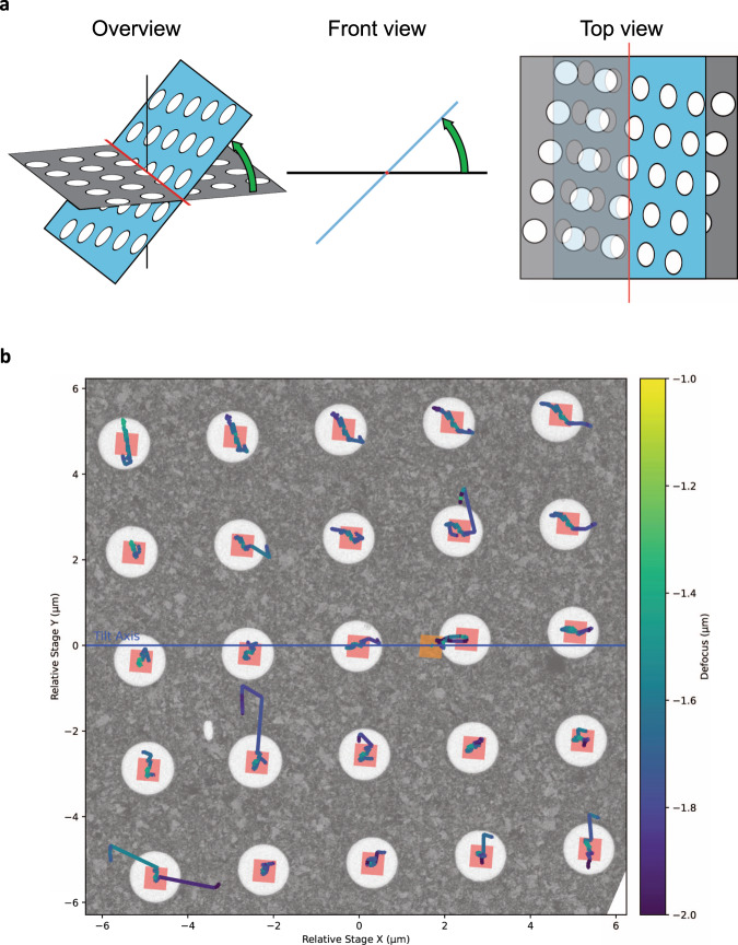
Fig. 1
Parallel acquisition of tilt-series using beam-image shift electron cryo-tomography (BISECT).
a Schematic of the movement of ROIs (white circles) from the initial position (gray) and after stage tilting (blue). b Evolution of the targeting and defocus over a 5u2009u00d7u20095-hole area. The in...
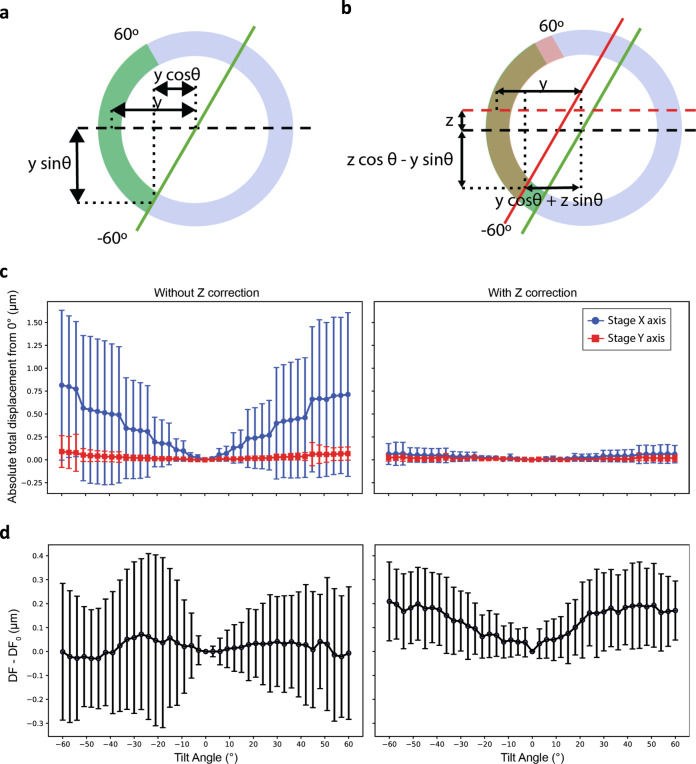
Fig. 2
Effects of eucentric plane correction during tilt-series acquisition.
a , b Comparison of the target displacement during tilting assuming that the sample is flat compared to the center of rotation ( a , green arc) or when considering an off-plane shift ( b , red arc and...
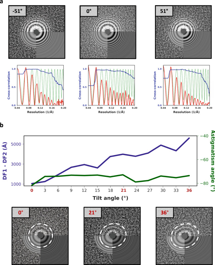
Fig. 3
Astigmatic tilted-CTF determination from low-dose tomographic tilt-series.
a 2D power spectra from projections at u221251u00b0, 0u00b0, and 51u00b0 from a tilt-series downloaded from EMPIAR-10453 (top) and corresponding fitted 1D models (bottom) showing radially averaged CTF...
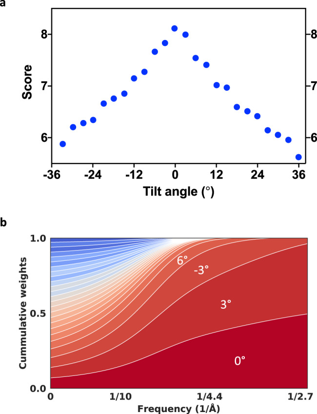
Fig. 4
Self-tuning exposure weighting based on assigned particle scores.
a Average similarity scores calculated over individual particle projections and plotted as a function of the tilt-angle revealing the expected characteristic of the dose-symmetric scheme showing highe...
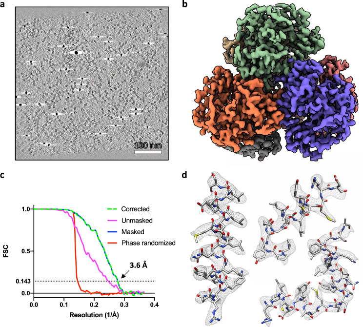
Fig. 5
Near-atomic resolution structure of 300u2009kDa complex using BISECT/CSPT.
a Representative 50 nm-thick slice through tomographic reconstruction showing individual dNTPase particles (a total of 64 tomograms were used). Scale bar 100u2009nm. b Overview of dNTPase map obtained...
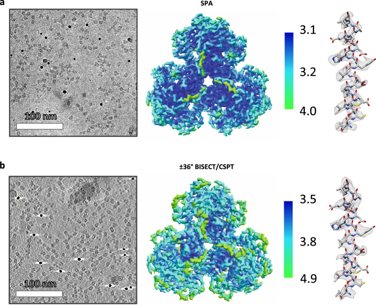
Fig. 6
Comparison of SPA and CET structures of dNTPase.
a Representative 2D micrograph selected out of a total of 64 images (left, scale bar 100u2009nm), SPA map colored according to local resolution (middle) and corresponding density for an alpha helix (r...
Figure images are served from the NIH/NLM PubMed Central Open Access Subset or Europe PMC; copyright remains with the publishers and authors.
💬 Discussion
0 commentsNo comments yet. Be the first to start a discussion!
Leave a Comment