Abstract
AbstractSuper-resolution microscopy (PALM, STORM etc.) provides a plethora of fluorescent signals in dense cellular environments which can be difficult to interpret. Here we describe ClusterViSu, a method for image reconstruction, visualization and quantification of labelled protein clusters, based on Voronoi tessellation of the individual fluorescence events. The general applicability of this clustering approach for the segmentation of super-resolution microscopy data, including for co-localization, is illustrated on a series of important biological objects such as chromatin complexes, RNA polymerase, nuclear pore complexes and microtubules.
🔬 Techniques
💻 Software
✨ Fluorophores
🧪 Sample Preparation
🔬 Cell Lines
🏭 Microscope Brands
🧪 Reagent Suppliers
📷 Detectors
🔎 Objectives
💻 Software Details
💻 Code & Software
💾 Data Repositories
🏛️ Research Organizations (ROR)
Affiliated research institutions:
📋 Methods
Super-resolution imaging
HeLa cells were plated in a 4-compartment glass-bottom petri dish (CELLView, Greiner Bio-One) and fixed with 4% formaldehyde for 20 min in phosphate-buffered saline solution (PBS). After permeabilization with 0.1% Triton in PBS (PBS/Tx) twice for 10 min, the primary antibody (anti-β-tubulin monoclonal (1Tub-2A2, in house IGBMC) was used as mouse ascites fluid diluted 500× in PBS/Tx; RNA Pol II monoclonal antibody (1PB-7C2, in house IGBMC), directed against the CTD of the largest subunit of RNA Pol II (RPB I) was used as a purified IgG at 5 μg/ml in PBS/Tx; histone H2B monoclonal antibody (LG11-2) was used as a 500× dilution of mouse ascites fluid in PBS/Tx) was incubated overnight at 4 °C. The sample was then washed with PBS/Tx three times over 2 hours, and the secondary antibody (goat anti-mouse Alexa Fluor-647 or Alexa Fluor-555 conjugated, Invitrogen) in dilution 4 μg/ml in PBS/Tx was incubated for 2 hours at room temperature. Subsequently, the cells were washed in PBS/Tx three times for 2 hours, then briefly three times in PBS. For the TPR sample, cells were cultured on coverslips and fixed in 4% paraformaldehyde for 10 min, permeabilized in 0.5% Triton for 10 min, blocked in 1% BSA for 30 min, and incubated with primary antibodies (TPR rabbit polyclonal antibody, Abcam, ab84516) for 1h and with secondary antibodies (goat anti-rabbit Alexa Fluor-647) for 45 min 14 . The double-labelled β-tubulin sample was mounted in an imaging buffer 31 that contained 20% of Vectashield (Vector Laboratories), 70% of 2,2′-thiodiethanol (also known as thiodiglycol or TDE) and 10% of PBS 10× (the measured refractive index of this mounting medium is 1.491). The H2B/RNA Pol II, the TPR and the β-tubulin sample used for Fig. 1 were mounted in a PBS buffer with addition of 10 mM of cysteamine (also known as β-mercaptoethylamine or MEA) and 25 mM of HEPES (pH 7.5). The super-resolution experiments were performed on a Leica SR GSD system built on a base of DMI6000 B inverted wide-field microscope. We used the HCX PL APO 100×/1.47 Oil CORR TIRF PIFOC objective with a 1.6× magnification lens that provides an equivalent pixel size of 100 nm on the Andor iXon3 DU-897U-CS0-#BV EMCCD camera with a field of view of 18 × 18 μm in super-resolution mode. Continuous wave fiber lasers (MPBC Inc., 488 nm 300 mW, 532 nm 1000 mW, 642 nm 500 mW) and a diode laser (405 nm 30 mW) were utilized for excitation. The microscope is also equipped with a suppressed motion (SuMo) sample stage, which reduces drift but does not eliminate it (typical values 20–50 nm over 10 min). The residual drift was corrected by data processing (see below). The samples were first illuminated with the 100% power of the appropriate laser to quickly send the fluorophores into the dark state. The acquisition started after beginning of observation of single-fluorophore events (“blinking”) that corresponded to the drop of the correlation value of consecutive frames to approximately 0.2 in the corresponding wizard in the LAS AF software. The time of exposition of a frame was 6.34 ms (H2B and RNA Pol II data) or 50 ms (β-tubulin and TPR data); the electron multiplying gain of the camera was 300 for H2B, RNA Pol II, TPR, 150 for β-tubulin-Alexa 647 and 63 for β-tubulin-Alexa 555; the laser power during the acquisition was 30% (H2B), 50% (TPR) or 100% (RNA Pol II and β-tubulin). After a few minutes, as the number of blinking evens dropped, the sample started to be illuminated additionally by a 405 nm laser with gradual increase of its intensity in order to keep a nearly constant rate of single-molecular returns into the ground state. The acquisition was stopped after almost complete bleaching of the fluorophore.
Show full methods section
Super-resolution imaging
HeLa cells were plated in a 4-compartment glass-bottom petri dish (CELLView, Greiner Bio-One) and fixed with 4% formaldehyde for 20 min in phosphate-buffered saline solution (PBS). After permeabilization with 0.1% Triton in PBS (PBS/Tx) twice for 10 min, the primary antibody (anti-β-tubulin monoclonal (1Tub-2A2, in house IGBMC) was used as mouse ascites fluid diluted 500× in PBS/Tx; RNA Pol II monoclonal antibody (1PB-7C2, in house IGBMC), directed against the CTD of the largest subunit of RNA Pol II (RPB I) was used as a purified IgG at 5 μg/ml in PBS/Tx; histone H2B monoclonal antibody (LG11-2) was used as a 500× dilution of mouse ascites fluid in PBS/Tx) was incubated overnight at 4 °C. The sample was then washed with PBS/Tx three times over 2 hours, and the secondary antibody (goat anti-mouse Alexa Fluor-647 or Alexa Fluor-555 conjugated, Invitrogen) in dilution 4 μg/ml in PBS/Tx was incubated for 2 hours at room temperature. Subsequently, the cells were washed in PBS/Tx three times for 2 hours, then briefly three times in PBS. For the TPR sample, cells were cultured on coverslips and fixed in 4% paraformaldehyde for 10 min, permeabilized in 0.5% Triton for 10 min, blocked in 1% BSA for 30 min, and incubated with primary antibodies (TPR rabbit polyclonal antibody, Abcam, ab84516) for 1h and with secondary antibodies (goat anti-rabbit Alexa Fluor-647) for 45 min 14 . The double-labelled β-tubulin sample was mounted in an imaging buffer 31 that contained 20% of Vectashield (Vector Laboratories), 70% of 2,2′-thiodiethanol (also known as thiodiglycol or TDE) and 10% of PBS 10× (the measured refractive index of this mounting medium is 1.491). The H2B/RNA Pol II, the TPR and the β-tubulin sample used for Fig. 1 were mounted in a PBS buffer with addition of 10 mM of cysteamine (also known as β-mercaptoethylamine or MEA) and 25 mM of HEPES (pH 7.5). The super-resolution experiments were performed on a Leica SR GSD system built on a base of DMI6000 B inverted wide-field microscope. We used the HCX PL APO 100×/1.47 Oil CORR TIRF PIFOC objective with a 1.6× magnification lens that provides an equivalent pixel size of 100 nm on the Andor iXon3 DU-897U-CS0-#BV EMCCD camera with a field of view of 18 × 18 μm in super-resolution mode. Continuous wave fiber lasers (MPBC Inc., 488 nm 300 mW, 532 nm 1000 mW, 642 nm 500 mW) and a diode laser (405 nm 30 mW) were utilized for excitation. The microscope is also equipped with a suppressed motion (SuMo) sample stage, which reduces drift but does not eliminate it (typical values 20–50 nm over 10 min). The residual drift was corrected by data processing (see below). The samples were first illuminated with the 100% power of the appropriate laser to quickly send the fluorophores into the dark state. The acquisition started after beginning of observation of single-fluorophore events (“blinking”) that corresponded to the drop of the correlation value of consecutive frames to approximately 0.2 in the corresponding wizard in the LAS AF software. The time of exposition of a frame was 6.34 ms (H2B and RNA Pol II data) or 50 ms (β-tubulin and TPR data); the electron multiplying gain of the camera was 300 for H2B, RNA Pol II, TPR, 150 for β-tubulin-Alexa 647 and 63 for β-tubulin-Alexa 555; the laser power during the acquisition was 30% (H2B), 50% (TPR) or 100% (RNA Pol II and β-tubulin). After a few minutes, as the number of blinking evens dropped, the sample started to be illuminated additionally by a 405 nm laser with gradual increase of its intensity in order to keep a nearly constant rate of single-molecular returns into the ground state. The acquisition was stopped after almost complete bleaching of the fluorophore.
Data processing
The localization and fitting of single-molecule events were performed in real time during acquisitions in Leica LAS AF 3.2.0.9652 software with the “center of mass” fitting method. To reduce the number of localizations of the same fluorophore and improve localization precision the data were processed by averaging the coordinates of consecutive events within a radius of 50 nm around each localization. Subsequently, the data were processed in SharpViSu (ref. 30 , in press; https://github.com/andronovl/SharpViSu ). The drift was detected and corrected using cross-correlation-based approach. Briefly, the dataset was divided on several consecutive subsets, from each of them a histogram image with pixelation of 20–40 nm was build, the shift between these images was detected with subpixel precision and interpolated linearly throughout intermediate frames. The shift was then subtracted from every frame. The procedure was repeated iteratively 4 times assuring absence of detectable residual drift. For correction for the chromatic aberrations, the aberrations were detected beforehand with Tetraspeck multi-color beads, interpolated through the field of view with 2-order polynomial functions and subtracted from the molecular coordinates obtained from either 488 nm or 532 nm imaging channels. Regions of interest (ROI) for Voronoi analysis were selected manually allowing faster computations and more homogeneous distributions compared to the entire field of view. The following analysis was performed in Matlab using customized code that is included as modules in the ClusterViSu software. Voronoi diagrams (vertices of polygons and connectivity order) were retrieved with either ‘voronoi’ or ‘voronoin’ functions. Areas of the cells were determined from the vertices with the function ‘polyarea’, the local density in each data point was defined as the inverse value of the area of the corresponding Voronoi polygon. To have a smooth appearance that can be used for visualization ( Fig. 1C–E ) or segmentation ( Fig. 2E,F ) the values of the local density were interpolated to a regular grid (pixels) using the ‘griddata’ function and the ‘natural’ interpolation method 32 . The spacing of the grid corresponds to the desired pixel size (in range of 2 to 20 nm in our case, it is indicated in the figure legends; at least 3–4 times smaller than the expected resolution to satisfy the Nyquist theorem). For the comparison of visualization techniques, we used a Gaussian distribution of points arranged as two parallel lines, with a distance of 40 nm between the centers of the distributions and the standard deviation of each distribution σ = 10 nm in the X direction ( Fig. 1A–D ). The linear density of localization in each line was 0.5 nm −1 . To this dataset we added localizations with random (x, y) coordinates, with overall density of 400 μm −2 , comparable to background density at experimental data. The photon counts for all events were distributed with Gaussian distribution around the mean value of 1000 photons with standard deviation of 300. This is similar to a procedure described by Baddeley et al. 4 with following modifications: linear densities were chosen to be similar to those of typical experimental data, noise was added, and single line profiles ( Fig. S1D ) were used along with projections ( Fig. 1D ; even though projections tend to not reflect discontinuities in the data, i.e. they generate back the underlying line structure). The Gaussian mode image was built representing each event as a Gaussian filter kernel with σ = A/(N ph ) 1/2 , where A = 240 nm (experimentally determined value for our system), and N ph is the number of photons. The FRC curves were calculated in 90 concentric rings (resulting in 90 frequency values in the FRC graphs) using the corresponding type of image representation for half-datasets 3 . For statistics, the FRC curves and the resolution values were calculated 50 times for each localization table, using different random separations of the dataset on two parts. Standard deviations of the obtained values are shown in error bar for each frequency point. The FRC curves for histogram, Gaussian and Voronoi representations were also calculated by the FSC program (Image Science Software GmbH) 33 confirming the results obtained with our method. The simulated cluster data on Fig. 2 were generated as randomly distributed points in circles with a radius of 50 nm. The density of points in the clusters was 3 · 10 −3 . The positions of clusters and of low-density (4 · 10 −4 ) background points were distributed randomly in the field of view (FOV). The distributions of the sizes of the Voronoi cells were built as histograms of the areas of the cells, for a range from 0 to 4 times the median value of the area, using 2N 1/3 bins, where N is the number of the polygons, excluding infinity-sized polygons at the boundaries of the ROI. For Monte-Carlo simulations, random coordinates were generated throughout the ROI using the ‘rand’ function. To obtain the confidence envelope, the distributions were generated for 50 different random sets of points, the boundaries of the envelope were determined as ± 1.96 σ for each bin of the histogram, where is the average number of cells within the range of the bin and σ is the standard deviation of n, calculated from the 50 random datasets. The abscissas of the first and the second intersections between the curves of the experimental and the mean value of the randomized distributions were determined from the two points around the intersections in the linear approximation. The Voronoi cells smaller than the area corresponding to the first intersection were kept, and all touching cells (those that have at least one common vertex) were combined together yielding vertices of clusters. The clusters were rasterized with the ‘poly2mask’ function using a pixel size of 1 nm. For the nuclear pore data a threshold was used to set the minimum number of events to remove small, spurious clusters. In our current implementation calculations for medium-sized datasets, e.g. Monte-Carlo simulations of 5⋅10 4 localizations, take around a minute; calculations may be parallelized in future software versions. The simulated data on Figs S3–S6 were generated as 10 × 10 clusters with radius of 50 nm through a FOV of 4 × 4 μm. The positions of the centers of the clusters were distributed regularly in the FOV. The points inside the clusters and in background were placed randomly with the indicated average density. For Fig. S3 the positions of the points were picked from the normal distribution using the mean defined at the previous step and the standard deviation of σ loc . For Figs S4 and S5 , n (number of re-localizations) points were picked for every original point using the normal distribution with the standard deviation σ loc = 10 nm and the mean value at the position of the original point. For Monte-Carlo simulations on Fig. S5 the randomized datasets were formed using N/n sim seeds at spatially random positions and distributing n sim points by Gaussian distribution with σ loc = 10 nm around the seeds; N is the number of points in the original dataset, n sim is the number of re-localizations used in the Monte-Carlo simulations. For segmented multi-color images, the co-localization value for a given species is defined by the ratio of the superposed area S between two colors relative to the total area of clusters of a given species. To compare the obtained values with overlapping area S rand of randomly distributed clusters we shuffled the experimentallydetermined clusters into randomized positions through the same field of view, independently for each color. Firstly, the list of cluster polygons was permutated randomly using Matlab’s ‘randperm’ function. Then, we determined the centroids of the clusters by formulas: , ; where C x , C y are the (x, y) coordinates of the centroid of a given polygon, x i , y i are the coordinates of the vertices, n is the number of the vertices, and the vertex i = 0 equals to the vertex i = n. A is the signed area of the polygon: . After subtraction of the centroid coordinates from coordinates of the vertices of the polygons, the new coordinates were determined as a random number situated in the FOV of the initial size. To avoid overlapping of newly placed clusters, we iteratively checked for each cluster being placed at a random spot if it was not overlapping with the previously placed clusters of the same color, in which case another random coordinate was chosen. The shuffling procedure was repeated 50 times with different random positions, and the 95% confidence range for the co-localization in the random case was obtained as mean ±1.96 σ of the corresponding ratios of the surfaces. Pair distribution functions were calculated using Matlab’s ‘pdist2’. For the nearest neighbor distance, the smallest pairwise distance value was chosen for each data point. The equivalent radius of a cluster was calculated as the radius of a circle with the same surface area as the cluster. Quantified properties of clusters (number of events, equivalent radius, nearest distance between neighboring clusters) are represented as mean ± standard deviation of the corresponding values.
📊 Figures
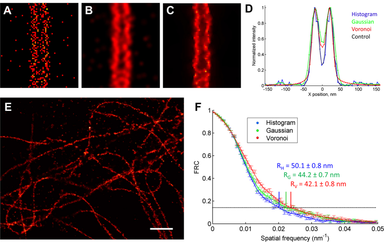
Figure 1
Comparison of different representation methods of localization events in super-resolution microscopy, showing that image representation by Voronoi diagrams fully preserves the resolution.
( A u2013 C ) Simulated images of two lines separated by 40u2009nm and composed of localization events with a standard deviation of 10u2009nm in histogram ( A ), Gaussian ( B ) and Voronoi-based inter...
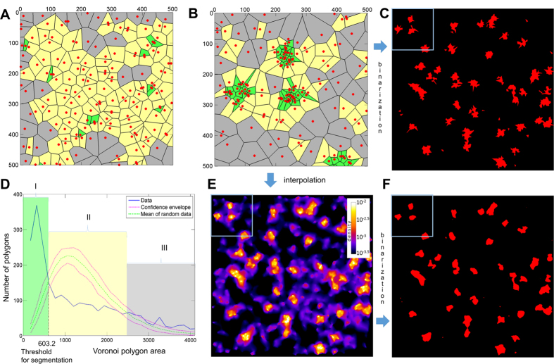
Figure 2
Principle of Voronoi-based image segmentation which allows visualization and quantification of clusters.
( A ) A region of simulated pointillist data with random distribution. ( B ) Simulated clustered distribution of the same number of points as in the random dataset. ( C ) Clustering obtained after dir...
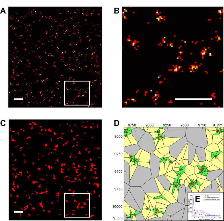
Figure 3
Segmentation and cluster analysis of nucleoporin protein TPR.
( A ) Histogram-based image reconstruction of TPR distribution at the nuclear envelope with a magnified region (white box) in ( B ). ( C ) Segmented Voronoi diagram calculated from the image in ( A ) ...
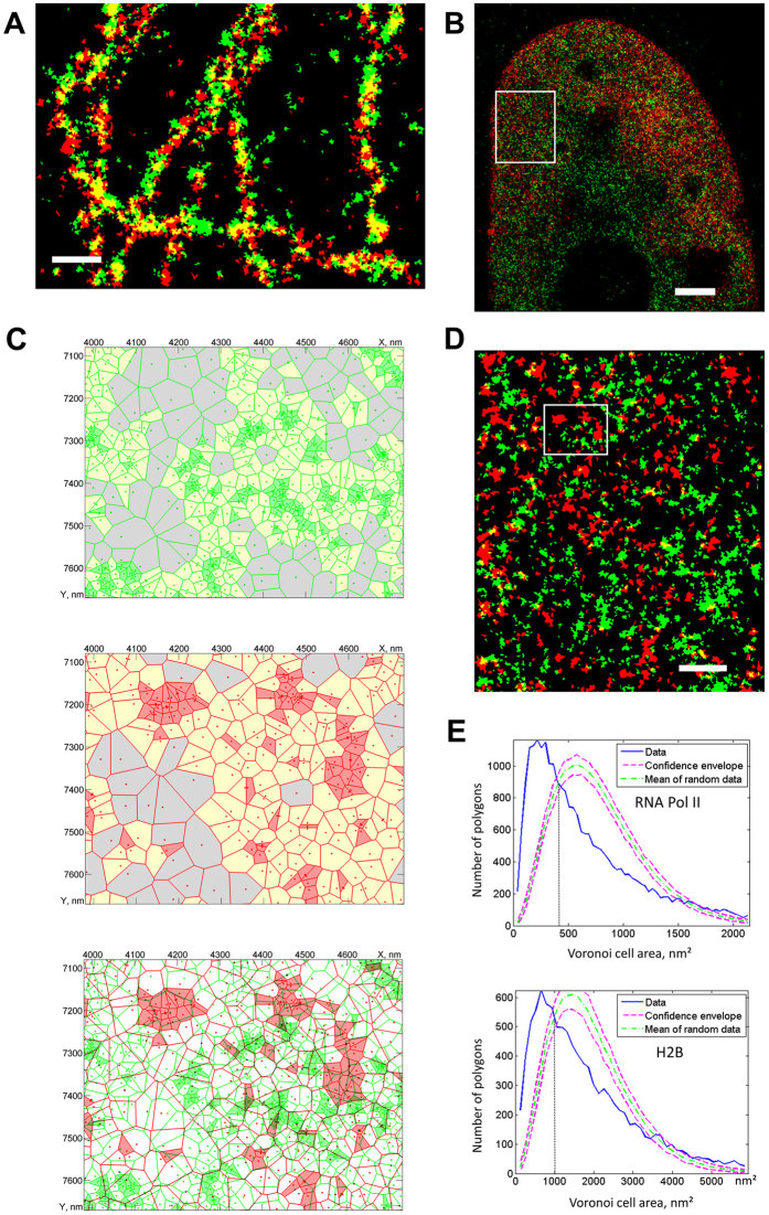
Figure 4
Co-localization analysis using Voronoi tessellations.
( A ) Segmented Voronoi diagram of u03b2-tubulin, labelled with two different fluorophores (Alexa Fluor-555, green, and Alexa Fluor-647, red) demonstrating strong co-localization (S/S red =u20090.416,...
Figure images are served from the NIH/NLM PubMed Central Open Access Subset or Europe PMC; copyright remains with the publishers and authors.
💬 Discussion
0 commentsNo comments yet. Be the first to start a discussion!
Leave a Comment