Abstract
AbstractIn pathological diagnostics, histological images highlight the oncological features of excised specimens, but they require laborious and costly staining procedures. Despite recent innovations in label-free microscopy that simplify complex staining procedures, technical limitations and inadequate histological visualization are still problems in clinical settings. Here, we demonstrate an interconnected deep learning (DL)-based framework for performing automated virtual staining, segmentation, and classification in label-free photoacoustic histology (PAH) of human specimens. The framework comprises three components: (1) an explainable contrastive unpaired translation (E-CUT) method for virtual H&E (VHE) staining, (2) an U-net architecture for feature segmentation, and (3) a DL-based stepwise feature fusion method (StepFF) for classification. The framework demonstrates promising performance at each step of its application to human liver cancers. In virtual staining, the E-CUT preserves the morphological aspects of the cell nucleus and cytoplasm, making VHE images highly similar to real H&E ones. In segmentation, various features (e.g., the cell area, number of cells, and the distance between cell nuclei) have been successfully segmented in VHE images. Finally, by using deep feature vectors from PAH, VHE, and segmented images, StepFF has achieved a 98.00% classification accuracy, compared to the 94.80% accuracy of conventional PAH classification. In particular, StepFF’s classification reached a sensitivity of 100% based on the evaluation of three pathologists, demonstrating its applicability in real clinical settings. This series of DL methods for label-free PAH has great potential as a practical clinical strategy for digital pathology.
🔬 Techniques
💻 Software
🧪 Sample Preparation
💻 Software Details
🏛️ Research Organizations (ROR)
Affiliated research institutions:
📋 Methods
Data preparation
All histopathological procedures were conducted following regulations and guidelines approved by the Institutional Review Board of POSTECH (approval no. PIRB-2019-E013). For specimen preparation, we harvested human liver tissue with hepatocellular carcinoma, along with adjacent noncancerous tissue. The excised tissue was processed into FFPE blocks. The 10 μm-thick unstained deparaffinized FFPE tissue sections were prepared for PA imaging. PAH images were then obtained with a UV-PAM system that uses an ultraviolet (266 nm) laser for label-free imaging (Fig. 2a ) 63 . Corresponding H&E-stained images were also acquired at approximately the same location as the PAH image acquisition. For segmentation, training the model requires data with nucleus contour label information for the PAH, H&E, and VHE images. However, obtaining such annotated data is inherently challenging, primarily due to its time-consuming and labor-intensive nature. Acquiring label information for the PAH and VHE images is especially difficult because there is little pathological knowledge to guide segmenting the nucleus contours. Therefore, instead of segmenting the nucleus contour information manually, we quickly trained and tested the model using public H&E datasets containing contour information. A total of four datasets were used to train the segmentation model: CPM-15 74 , CPM-17 74 , Kumar 75 , and TNBC 76 .
Image pre-processing and post-processing
In the pre-processing step for raw PAH images, we conducted contrast adjustment, denoising, and background erasing. For the subsequent DL training processes, WSIs of H&E slides were converted to the same size as PAH images and cropped into smaller image tiles. First, the ×20 H&E images were downsampled to match at the magnification of ×10, which is the scale of the PAH images. The PAH images were then inverted to match the background color of the downsampled H&E image (the background was set to white). For training and testing, WSIs of both H&E and PAH images were cropped into small image tiles of 512 × 512 pixels with 50% overlap. For both virtual staining and classification, these image tiles were divided into training and test sets in proportions of 5:1. On the other hand, for segmentation, we used publicly available datasets 74 – 76 and cropped them to 224 × 224 pixels for training. All the tiles of PAH, H&E, and VHE images were employed as test data for the segmentation model. A fivefold cross-validation was employed to validate the segmentation and classification results. For testing, we have used altogether different tiles, which had never been used during the training phase. We also organized the test dataset to balance between cancer and non-cancer cases for classification. Additionally, since PAH and H&E images have different numbers of channels and E-CUT requires the same number of channels for the input and ground truth, 1-channel grayscale PAH images were stacked and converted to three-channel PAH images. The final post-processing step was to stitch the small image tiles to get the original WSI. We merged them considering the 50% overlap, so that the results were summed up, and the overlapping sections were divided by the number of overlapping images.
Show full methods section
Data preparation
All histopathological procedures were conducted following regulations and guidelines approved by the Institutional Review Board of POSTECH (approval no. PIRB-2019-E013). For specimen preparation, we harvested human liver tissue with hepatocellular carcinoma, along with adjacent noncancerous tissue. The excised tissue was processed into FFPE blocks. The 10 μm-thick unstained deparaffinized FFPE tissue sections were prepared for PA imaging. PAH images were then obtained with a UV-PAM system that uses an ultraviolet (266 nm) laser for label-free imaging (Fig. 2a ) 63 . Corresponding H&E-stained images were also acquired at approximately the same location as the PAH image acquisition. For segmentation, training the model requires data with nucleus contour label information for the PAH, H&E, and VHE images. However, obtaining such annotated data is inherently challenging, primarily due to its time-consuming and labor-intensive nature. Acquiring label information for the PAH and VHE images is especially difficult because there is little pathological knowledge to guide segmenting the nucleus contours. Therefore, instead of segmenting the nucleus contour information manually, we quickly trained and tested the model using public H&E datasets containing contour information. A total of four datasets were used to train the segmentation model: CPM-15 74 , CPM-17 74 , Kumar 75 , and TNBC 76 .
Image pre-processing and post-processing
In the pre-processing step for raw PAH images, we conducted contrast adjustment, denoising, and background erasing. For the subsequent DL training processes, WSIs of H&E slides were converted to the same size as PAH images and cropped into smaller image tiles. First, the ×20 H&E images were downsampled to match at the magnification of ×10, which is the scale of the PAH images. The PAH images were then inverted to match the background color of the downsampled H&E image (the background was set to white). For training and testing, WSIs of both H&E and PAH images were cropped into small image tiles of 512 × 512 pixels with 50% overlap. For both virtual staining and classification, these image tiles were divided into training and test sets in proportions of 5:1. On the other hand, for segmentation, we used publicly available datasets 74 – 76 and cropped them to 224 × 224 pixels for training. All the tiles of PAH, H&E, and VHE images were employed as test data for the segmentation model. A fivefold cross-validation was employed to validate the segmentation and classification results. For testing, we have used altogether different tiles, which had never been used during the training phase. We also organized the test dataset to balance between cancer and non-cancer cases for classification. Additionally, since PAH and H&E images have different numbers of channels and E-CUT requires the same number of channels for the input and ground truth, 1-channel grayscale PAH images were stacked and converted to three-channel PAH images. The final post-processing step was to stitch the small image tiles to get the original WSI. We merged them considering the 50% overlap, so that the results were summed up, and the overlapping sections were divided by the number of overlapping images.
Explainable contrastive unpaired translation network Network architectures and training
We adopted a CUT 57 architecture for the E-CUT model to learn the unpaired image translation between label-free PAH images and corresponding histological images stained with H&E (Fig. 3a ). The generator network for E-CUT, inspired by the ResNet model, consists of downsampling, residual blocks, and up-sampling parts 89 . The downsampling process encodes an input image down to the 9 residual blocks. Each residual block is designed with a skip connection where an input to the block is concatenated to an output of the block, enabling interpretation of the encoding. In the residual block, a padded convolutional layer keeps the image size constant. The residual blocks are followed by up-sampling to decode the representation to match the size of a final output image. For the discriminator network, we utilized a PatchGAN classifier 90 . This patch-level discriminator can determine whether 70 × 70 overlapping patches are real or fake, and it can be used on images of any size in a fully convolutional fashion. The final output of the discriminator is defined as the average of the classification results on all patches. The patch information from PAH (the input) is trained to transform it into the style of the H&E (the ground truth). In particular, during the training process, our model stores the saliency mask and integrated gradients attribution map at each training step to improve explainability. To obtain the integrated gradients, we approximate the gradient integral of the discriminator model output over the input along the path to compute the importance score for each input feature. In order to obtain the attribution map, a total of 50 steps of approximation are performed using Pytorch’s captum library 91 . Finally, the trained model is used to virtually stain the test data. The training data (PAH and H&E) and virtually stained data (VHE) are reserved for use in later stages (segmentation and classification). Loss function To ensure a reliable image translation between PAH images (the source, X ) and H&E images (the target, Y ), it is important to define a loss function. The goal of virtual staining is to transform the input data into the target’s style, color, and shape. However, at the same time, details such as information about cell nuclei should be preserved. Therefore, as the final training loss, we used an equal combination of the adversarial, PatchNCE, and saliency losses (Fig. 3a ). Adversarial loss ( documentclass[12pt]{minimal} usepackage{amsmath} usepackage{wasysym} usepackage{amsfonts} usepackage{amssymb} usepackage{amsbsy} usepackage{mathrsfs} usepackage{upgreek} setlength{oddsidemargin}{-69pt} begin{document}$${{rm{l}}}_{{adv}}$$end{document} l adv ) minimizes the differences between the output of each network and the target domain image 92 . Contrastive learning with PatchNCE loss ensures that learning proceeds in a way that maximizes the mutual information between the input and output image patches 57 , which are obtained by passing the input and output images through a generator encoder. PatchNCE loss is calculated as the average of documentclass[12pt]{minimal} usepackage{amsmath} usepackage{wasysym} usepackage{amsfonts} usepackage{amssymb} usepackage{amsbsy} usepackage{mathrsfs} usepackage{upgreek} setlength{oddsidemargin}{-69pt} begin{document}$${{rm{l}}}_{{PatchNCE}}(X)$$end{document} l PatchNCE ( X ) on images from domain documentclass[12pt]{minimal} usepackage{amsmath} usepackage{wasysym} usepackage{amsfonts} usepackage{amssymb} usepackage{amsbsy} usepackage{mathrsfs} usepackage{upgreek} setlength{oddsidemargin}{-69pt} begin{document}$$X$$end{document} X and documentclass[12pt]{minimal} usepackage{amsmath} usepackage{wasysym} usepackage{amsfonts} usepackage{amssymb} usepackage{amsbsy} usepackage{mathrsfs} usepackage{upgreek} setlength{oddsidemargin}{-69pt} begin{document}$${{rm{l}}}_{{PatchNCE}}(Y)$$end{document} l PatchNCE ( Y ) on images from domain documentclass[12pt]{minimal} usepackage{amsmath} usepackage{wasysym} usepackage{amsfonts} usepackage{amssymb} usepackage{amsbsy} usepackage{mathrsfs} usepackage{upgreek} setlength{oddsidemargin}{-69pt} begin{document}$$Y$$end{document} Y , where documentclass[12pt]{minimal} usepackage{amsmath} usepackage{wasysym} usepackage{amsfonts} usepackage{amssymb} usepackage{amsbsy} usepackage{mathrsfs} usepackage{upgreek} setlength{oddsidemargin}{-69pt} begin{document}$${{rm{l}}}_{{PatchNCE}}(X)$$end{document} l PatchNCE ( X ) ensures that the input-output patches correspond, and documentclass[12pt]{minimal} usepackage{amsmath} usepackage{wasysym} usepackage{amsfonts} usepackage{amssymb} usepackage{amsbsy} usepackage{mathrsfs} usepackage{upgreek} setlength{oddsidemargin}{-69pt} begin{document}$${{rm{l}}}_{{PatchNCE}}(Y)$$end{document} l PatchNCE ( Y ) serves to further prevent the generator from making unnecessary changes. The saliency loss ( documentclass[12pt]{minimal} usepackage{amsmath} usepackage{wasysym} usepackage{amsfonts} usepackage{amssymb} usepackage{amsbsy} usepackage{mathrsfs} usepackage{upgreek} setlength{oddsidemargin}{-69pt} begin{document}$${{rm{l}}}_{{Saliency}}(X,Y)$$end{document} l Saliency ( X , Y ) ) is the L1 loss between documentclass[12pt]{minimal} usepackage{amsmath} usepackage{wasysym} usepackage{amsfonts} usepackage{amssymb} usepackage{amsbsy} usepackage{mathrsfs} usepackage{upgreek} setlength{oddsidemargin}{-69pt} begin{document}$${{rm{X}}}_{{saliency}}$$end{document} X saliency and documentclass[12pt]{minimal} usepackage{amsmath} usepackage{wasysym} usepackage{amsfonts} usepackage{amssymb} usepackage{amsbsy} usepackage{mathrsfs} usepackage{upgreek} setlength{oddsidemargin}{-69pt} begin{document}$${{rm{Y}}}_{{saliency}}$$end{document} Y saliency , and it is employed to preserve similar saliency masks during transformation and to improve explainability by visualizing the saliency mask 52 . In addition to adversarial and PatchNCE losses, saliency loss is used to extract the saliency mask of the input and the generated output to check whether the structural information is well preserved during training and leads to more accurate results. The saliency losses for the source and target domains are obtained by these equations: 1 documentclass[12pt]{minimal} usepackage{amsmath} usepackage{wasysym} usepackage{amsfonts} usepackage{amssymb} usepackage{amsbsy} usepackage{mathrsfs} usepackage{upgreek} setlength{oddsidemargin}{-69pt} begin{document}$${X}_{{saliency}}=1-{sigmoid}left(left(X-{X}_{{threshold}}right)* 100right)$$end{document} X saliency = 1 − sigmoid X − X threshold * 100 2 documentclass[12pt]{minimal} usepackage{amsmath} usepackage{wasysym} usepackage{amsfonts} usepackage{amssymb} usepackage{amsbsy} usepackage{mathrsfs} usepackage{upgreek} setlength{oddsidemargin}{-69pt} begin{document}$${Y}_{{saliency}}=1-{sigmoid}left(left(Y-{Y}_{{threshold}}right)* 100right)$$end{document} Y saliency = 1 − sigmoid Y − Y threshold * 100 The detailed process of obtaining a saliency mask can be seen in Fig. S 4 . To consider only the saliency information, we first convert Y with RGB information to grayscale data by averaging the three-channel information, then apply sigmoid to both X and Y to get the saliency information. In the last step, the image is inversed to make the saliency information equal to 1. The optimal thresholds were obtained manually through experimentation, with 90 as the X threshold , which yields a good saliency mask for both noncancerous and cancerous cases of PAH, and 170 as the Y threshold , which works well for both noncancerous and cancerous cases of VHE (Fig. S 5 ). Finally, the entire loss function was formulated as 3 documentclass[12pt]{minimal} usepackage{amsmath} usepackage{wasysym} usepackage{amsfonts} usepackage{amssymb} usepackage{amsbsy} usepackage{mathrsfs} usepackage{upgreek} setlength{oddsidemargin}{-69pt} begin{document}$${{l}_{E-{CUT}}=l}_{{adv}}left(X,Yright)+frac{{l}_{{PatchNCE}}left(Xright)+{l}_{{PatchNCE}}left(Yright)}{2}+{l}_{{Saliency}}(X,Y)$$end{document} l E − CUT = l adv X , Y + l PatchNCE X + l PatchNCE Y 2 + l Saliency ( X , Y ) Parameter setting and evaluation metrics The Adam 93 optimizer, with b1 = 0.5 and b2 = 0.999, was used to optimize the E-CUT network parameters. The model was trained for 400 epochs, with an initial learning rate of 0.0002 for the first 200 epochs and a linear decay to a zero learning rate for the next 200 epochs, with 1 mini-batch setting. During the training phase, we augmented the data with horizontal flips. In terms of time consumption, E-CycleGAN took 73,800 s for the train and 60 s for the test, while E-CUT took relatively less time, ~62,400 s for the train and 33 s for the test. The overall test time of our proposed virtual staining (E-CUT) is much faster than the staining time of a human expert (20–30 minutes). For a fair comparison, the same configurations were used for other virtual staining models, i.e., CycleGAN, E-CycleGAN, and CUT. We used FID and KID to evaluate the virtual staining quality of the unpaired resultant image tiles. Lower values for both metrics indicate that the distributions of the two data are closer, indicating better virtual staining quality.
U-Net-based feature segmentation network
To numerically represent the characteristics of the VHE, we segment the cell nuclei information through feature segmentation and present it as three features: cell area, cell count, and mean intercellular distance.
Network architectures and training
This study employs the most well-known segmentation model, U-Net, which consists of contraction and expansion paths 73 (Fig. 4a ). While expansion paths have several deconvolution layers to upsample data and produce pixel-wise segmentation, contraction paths use convolution layers to produce high-level features in downsampling. Additionally, skip connections restore the spatial information lost during the downsampling. For feature segmentation, we employed four downscaling and four upscaling layers. In the training phase, we trained the model to segment cell nuclei information using a public dataset, and in the testing phase, we used the trained model to segment the cell nuclei information of PAH, VHE, and H&E images. Finally, the segmented cell nuclei information was analyzed using the OpenCV tool 77 (findContours, minEnclosingCircle) to obtain the cell area, cell count, and mean distance between cell nuclei for each tile. The cell area is the average value of the cell nuclei size, the cell count is the number of cell nuclei, and the mean intercellular distance is the average distance between cell nuclei. Parameter setting and evaluation metrics The U-Net-based segmentation model used Adam optimizer with b1 = 0.9 and b2 = 0.999, a learning rate of 0.0001, and a mini-batch size of 64, and was trained for 300 epochs. We used a combination of binary cross entropy and dice losses and allowed the training to stop early, depending on the validation loss 94 . We also used horizontal and vertical flips in the training phase to augment the data. In the last test phase, test time augmentation (TTA) was applied to get more accurate segmentation information. To visualize the results, we used the data visualization package Plotly 95 to plot 3D spatial scatter plots and box plots (Fig. 4c, d ). The total training time for the 5-fold cross-validation of feature segmentation took ~1300 s, and the test took a total of 165 s.
Stepwise feature fusion classification network Network architectures and training
In applying our StepFF method, we used the ResNet-18 model 79 as the base model for classification (Fig. 5a ). The 1-channel PAH image and the 3-channel VHE image were processed separately through ResNet-18 and processed into a fully connected layer to obtain 16-dimensional DFV from each. After that, to generate segmentation DFV from the previous feature segmentation results, three features (cell area, cell count, and distance) each from PAH and VHE were normalized with the mean and standard deviation of each segmented feature. Then, the same 16-dimensional DFV was generated using a fully connected layer with the normalized three biological features. Finally, we concatenated the three types of 16-dimensional DFVs into a 48-dimensional DFV and passed them through the last fully connected layer to classify the final non-cancer and cancer information. To compare the DL classification results with different source feature inputs (Table S6 ), we used a single ResNet for a single modality image (e.g., H&E, PAH, and VHE), and two ResNets for multiple modality images (e.g., PAH⊕VHE). After using ResNet to obtain DFVs, we used fully connected layers in the same way as StepFF to obtain the final cancer classification results.
Parameter setting and evaluation metrics
For the classification, we used the Adam optimizer to train the model for 1000 epochs, with b1 = 0.9 and b2 = 0.999, with a learning rate of 0.0001 and a mini-batch size of 32. We used focal loss for the imbalance data and allowed the training to terminate early based on the validation loss. We also used horizontal and vertical flips in the training phase to augment the data. The classification results were evaluated in terms of their accuracy, F1 score, precision, and recall. The fivefold cross-validation for StepFF took a total of 6000 s of training time and 16 s of testing time. For further analysis, we combined the results from each tile to create one large WSI cancerous probability map, which showed the overall cancerous classification results (Fig. 5c ). For this cancerous probability map, both training and test data tiles were used, in the following order. First, for each tile, StepFF’s cancerous prediction result was represented as a value between 0 and 1 and color-mapped (1 to purple, 0 to blue). Then, each tile was combined and reconstructed into the original WSI by using the post-processing method introduced in the image pre-processing & post-processing part.
Pathologists’ evaluation
To compare StepFF’s results with clinical diagnoses, we compared them with three pathologists’ evaluation (Fig. 5d ). We randomly shuffled 100 virtual staining results from StepFF together with a second group of 100 H&E images, then presented them all to three pathologists for evaluation at the same time. The pathologists were asked to determine whether each tile was noncancerous or cancerous according to the World Health Organization’s histological grading system for HCC. Five tiles with tissue coverages of 20% or less, which made the determination difficult, were excluded from the evaluation (Table S7 ). To measure the inter-pathologist agreement, we measured the kappa coefficient 85 , which is -1 for complete disagreement and 1 for complete agreement. Implementation details The image pre-processing steps were implemented in MATLAB using R2021a (The MathWorks Inc.). All the virtual staining, segmentation, and classification sequences were implemented using Python, version 3.8.12, and Pytorch, version 1.11.0. We implemented this training and testing on a Linux system with one Nvidia GeForce RTX 3090 GPU, an AMD EPYC 7302 CPU, and 346GB of RAM.
Supplementary information Supplementary information
📊 Figures
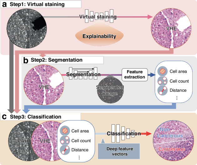
Fig. 1
DL-based framework for automated HIA to perform virtual staining, segmentation, and classification of label-free PAH.
a Virtual staining sequence with explainability to generate VHE images with label-free PAH. PAH photoacoustic histology image; and VHE virtual staining H&E. b Segmentation sequence to generate feature...
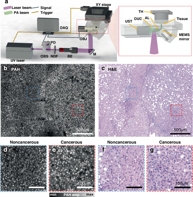
Fig. 2
Label-free PAH imaging system.
a Schematic of the PAH system and the close-up of the signal acquisition module. PD photodiode, OBS optical beam splitter, NDF neutral density filter, BE beam expander, M Mirror, OBJ objective lens, O...
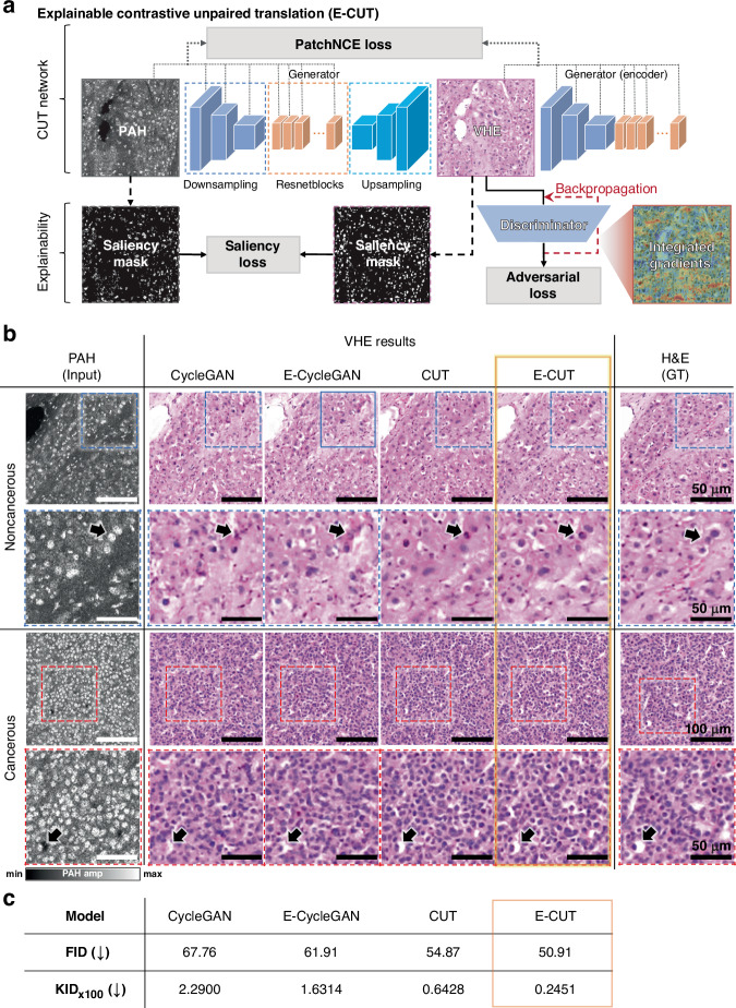
Fig. 3
Overall virtual staining network architecture and results.
a Explainable contrastive unpaired translation (E-CUT) network architecture. b Visual comparison of PAH (input), and VHE results with various networks: CycleGAN, explainable CycleGAN (E-CylcleGAN), CU...
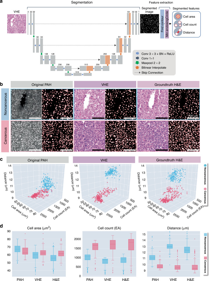
Fig. 4
Overall feature segmentation network architecture and results.
a U-Net-based feature segmentation network architecture with two phases: segmentation and feature extraction. b Segmentation of cell nuclei in PAH, VHE, and H&E images. Scale bars, 100u2009u03bcm. c 3...
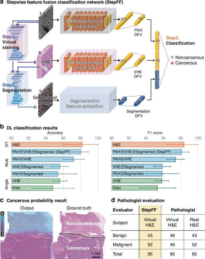
Fig. 5
Overall classification network architecture and results.
a Overall stepwise feature fusion (StepFF) classification network architecture. b Visualization of DL classification results for different source feature inputs. c Cancerous probability outputs of Ste...
Figure images are served from the NIH/NLM PubMed Central Open Access Subset or Europe PMC; copyright remains with the publishers and authors.
💬 Discussion
0 commentsNo comments yet. Be the first to start a discussion!
Leave a Comment