Abstract
Abstract Monitoring the proteins and lipids that mediate all cellular processes requires imaging methods with increased spatial and temporal resolution. STED (stimulated emission depletion) nanoscopy enables fast imaging of nanoscale structures in living cells but is limited by photobleaching. Here, we present event-triggered STED, an automated multiscale method capable of rapidly initiating two-dimensional (2D) and 3D STED imaging after detecting cellular events such as protein recruitment, vesicle trafficking and second messengers activity using biosensors. STED is applied in the vicinity of detected events to maximize the temporal resolution. We imaged synaptic vesicle dynamics at up to 24 Hz, 40 ms after local calcium activity; endocytosis and exocytosis events at up to 11 Hz, 40 ms after local protein recruitment or pH changes; and the interaction between endosomal vesicles at up to 3 Hz, 70 ms after approaching one another. Event-triggered STED extends the capabilities of live nanoscale imaging, enabling novel biological observations in real time.
🔬 Techniques
🔭 Microscopes
💻 Software
✨ Fluorophores
🧪 Sample Preparation
🔬 Cell Lines
🏭 Microscope Brands
🧪 Reagent Suppliers
📷 Detectors
💻 Software Details
💻 Code & Software
ImSwitch is a software solution in Python that aims at generalizing microscope control by providing a solution for flexible control...
A version of ImSwitch used for event-triggered STED imaging.
Generalization, including simulation, of the event-triggered widget provided in ImSwitch, for implementation in other python-based microscope control software.
💾 Data Repositories
🏷️ Research Resource Identifiers (RRIDs)
Verified research resources used in this paper:
🏛️ Research Organizations (ROR)
Affiliated research institutions:
📋 Methods
Microscopy set-up All images were acquired on a custom-built STED and widefield set-up, based on a STED set-up previously described 5 . A complete schematic and list of components is given in Supplementary Fig. 2 and Supplementary Note 10 . For STED, excitation of red-shifted dyes was done with a pulsed diode laser at 640 nm (pulse width 60 ps, LDH-D-C-640, PicoQuant). Depletion was done with a pulsed 775 nm laser beam (pulse width 530 ps, KATANA 08 HP, OneFive). Control of excitation and depletion laser illumination is done using an acousto-optic tunable filter (AOTFnC-400.650-TN + MPDS4C-B66–22–74.156, AA Opto Electronic) and an acousto-optic modulator (MT110-B50A1.5-IR-Hk + MDS1C-B65–34–85.135-RS, AA Opto Electronic). Orthogonal polarizations of the depletion beam are shaped using vortex and top-hat phase masks on a polarization-sensitive spatial light modulator (LCOM-SLM X10468 –02, Hamamatsu), and the polarization directions are temporally delayed to avoid interference. Wave plates are used to create circular polarization necessary for optimal depletion focus formation. Galvanometer mirrors are used for scanning (6215H + 671215HHJ-1, Cambridge Technology) in a scanning system to enable constant resolution across an 80 × 80 μm 2 field of view, as previously described 5 . Fluorescence is decoupled with a dichroic mirror. A bandpass filter (GT670/40m, Chroma) and a notch filter (NF03–785E-25, Semrock) are used before detection with an avalanche photodiode (SPCM-AQRH-13-TR, Excelitas Technologies). For the widefield set-up, excitation of blue-shifted fluorophores was done with a modulated 488 nm continuous-wave diode laser (06-MLD 488 nm, Cobolt). Detection of widefield images was done through a bandpass filter (FF01–540/80–25, Semrock) and a notch filter (ZET785NF, Chroma) with an sCMOS (scientific complementary metal oxide semiconductor) camera (Orca Flash 4.0, Hamamatsu). The widefield path is coupled into the beam path with a dichroic mirror after the scanning system. The general set-up uses a ×100/1.40 oil immersion objective (HC PL APO ×100/1.40 Oil STED White, Leica) and a microscope stand (DMi8, Leica). The system uses a mechanical stage for lateral sample movement (SCAN IM 130×85, Märzhäuser) and a piezostage for axial sample movement (LT-Z-100, Piezoconcept).
Show full methods section
Microscopy set-up All images were acquired on a custom-built STED and widefield set-up, based on a STED set-up previously described 5 . A complete schematic and list of components is given in Supplementary Fig. 2 and Supplementary Note 10 . For STED, excitation of red-shifted dyes was done with a pulsed diode laser at 640 nm (pulse width 60 ps, LDH-D-C-640, PicoQuant). Depletion was done with a pulsed 775 nm laser beam (pulse width 530 ps, KATANA 08 HP, OneFive). Control of excitation and depletion laser illumination is done using an acousto-optic tunable filter (AOTFnC-400.650-TN + MPDS4C-B66–22–74.156, AA Opto Electronic) and an acousto-optic modulator (MT110-B50A1.5-IR-Hk + MDS1C-B65–34–85.135-RS, AA Opto Electronic). Orthogonal polarizations of the depletion beam are shaped using vortex and top-hat phase masks on a polarization-sensitive spatial light modulator (LCOM-SLM X10468 –02, Hamamatsu), and the polarization directions are temporally delayed to avoid interference. Wave plates are used to create circular polarization necessary for optimal depletion focus formation. Galvanometer mirrors are used for scanning (6215H + 671215HHJ-1, Cambridge Technology) in a scanning system to enable constant resolution across an 80 × 80 μm 2 field of view, as previously described 5 . Fluorescence is decoupled with a dichroic mirror. A bandpass filter (GT670/40m, Chroma) and a notch filter (NF03–785E-25, Semrock) are used before detection with an avalanche photodiode (SPCM-AQRH-13-TR, Excelitas Technologies). For the widefield set-up, excitation of blue-shifted fluorophores was done with a modulated 488 nm continuous-wave diode laser (06-MLD 488 nm, Cobolt). Detection of widefield images was done through a bandpass filter (FF01–540/80–25, Semrock) and a notch filter (ZET785NF, Chroma) with an sCMOS (scientific complementary metal oxide semiconductor) camera (Orca Flash 4.0, Hamamatsu). The widefield path is coupled into the beam path with a dichroic mirror after the scanning system. The general set-up uses a ×100/1.40 oil immersion objective (HC PL APO ×100/1.40 Oil STED White, Leica) and a microscope stand (DMi8, Leica). The system uses a mechanical stage for lateral sample movement (SCAN IM 130×85, Märzhäuser) and a piezostage for axial sample movement (LT-Z-100, Piezoconcept).
Microscope control and computer
Microscope hardware control is mainly performed through a National Instruments data acquisition (NI-DAQ) acquisition board (PCIe-6353, National Instruments). Hardware is controlled using microscope control software ImSwitch 19 written in Python. Control of the etSTED method is performed using a custom-written widget and controller in ImSwitch, available at GitHub ( https://github.com/kasasxav/ImSwitch and https://github.com/jonatanalvelid/ImSwitch-etSTED ), which controls lasers, image acquisition, and runs real-time analysis pipelines with customizable parameters. Instructions on how to run etSTED imaging can be found in the GitHub repository of the standalone widget ( https://github.com/jonatanalvelid/etSTED-widget ), while instructions on how to run ImSwitch can be found in the repository on GitHub and corresponding documentation ( https://imswitch.readthedocs.io ). A focus lock controlled with ImSwitch combining an infrared laser (CP980S, Thorlabs), a CMOS camera (DMK 33UP1300, The Imaging Source) and the z -piezostage through a feedback loop, as previously described 5 , is used. It enables experiments to run stably for time periods longer than hours. The microscope control computer contains a Ryzen 7 3700X CPU (AMD) and a GeForce RTX 3060 Ti GPU (ASUS). etSTED widget and real-time image analysis pipelines The etSTED widget is a software module built in a generalized way to enable free choice of the lasers and detectors controlled with ImSwitch. For a thorough description of how to perform etSTED experiments with the control software, see the ImSwitch-etSTED GitHub repository readme file. The widget enables any arbitrary analysis pipeline to be used, and it additionally enables calibration of the imaging space coordinate transform. The coordinate transformation calibration is performed in a help widget into which a pre-acquired widefield image and scanning image of the same sample area can be loaded. Manual annotation of the same sample points in the images prepares fixed points for the coordinate transform calibration. A general third-order polynomial transformation with Levenberg–Marquart optimization is used, enabling it to be compatible and precise regardless of any aberrations and distortions that may be present in the optical paths. Afterwards, an image analysis pipeline can be loaded, and all editable parameters of the pipeline will be loaded into the GUI (graphical user interface). Last, to prepare for an etSTED experiment to be run, a binary mask of the sample may be recorded. It is performed with a separate functionality in which 10 frames are recorded and averaged, and a global thresholding is performed with a user-provided intensity threshold. The etSTED experiment is then started, with various options present as choices in the GUI: perform it as an endless loop or a single trigger; in visualization mode with real-time visualization of the preprocessed images to optimize analysis pipeline parameters; or in validation mode without triggering scans. While running etSTED experiments, detected event coordinates will be overlaid on the displayed widefield frames. The triggered imaging will be performed using pre-determined scanning parameters, including the choice of which lasers to use. Real-time analysis pipelines are provided as standalone python functions and must take the current widefield image, the previous widefield images and a binary mask of the considered region as input, and return a list of detected event coordinates in the widefield space. The real-time analysis pipeline additionally takes and returns a variable with any user-defined information from the analysis runs of the previous frames, for example for pipelines requiring tracking. It can additionally take any numerical parameters as input, for example various thresholds. The analysis pipelines developed in this work are provided and explained in more detail below, in Supplementary Notes 1 – 3 , as well as in the GitHub repository of the standalone widget ( https://github.com/jonatanalvelid/etSTED-widget ). Analysis pipeline parameter values used for each experiment are listed in Supplementary Table 1 . The etSTED widget and analysis pipelines in the control software use the Python packages numpy 45 , scipy 46 , cupy, opencv, trackpy 47 , pandas 48 , napari ( www.napari.org ) and pyqtgraph.
Rapid signal spikes image analysis pipeline
One analysis pipeline used throughout this work, rapid_signal_spikes, was developed to detect calcium events with Oregon Green 488 BAPTA-1 labeling in hippocampal neurons as well as CD63-pHluorin signal peaks in HeLa cells. It is shown schematically in Supplementary Fig. 1 , further described in Supplementary Note 1 , and available in the GitHub repository of the standalone widget ( https://github.com/jonatanalvelid/etSTED-widget/blob/main/analysis_pipelines/rapid_signal_spikes.py ). Although it is optimized for the above-mentioned biosensors, it is also likely to perform well with similar, fast fluorescence sensors after pipeline parameter tweaking. The pipeline consists of pre-processing that uses the current frame, the previous frame, and a binary region-of-interest mask; and peak detection. The pre-processing transforms the current image into a smoothed map comparing the intensity in each pixel between the current and previous image. The peak detection compares the image with a maximum-filtered version of itself, finding local maxima as the coordinates where the two are equal. To avoid detection of noise fluctuations, the coordinate intensities are thresholded. Finally, the ratiometrically brightest peak is used throughout this work as the coordinate where the triggered STED imaging takes place. Most of the analysis pipeline runs on the GPU, significantly decreasing the runtime as compared with running it on the CPU. Altogether, the analysis pipeline runs in 6 ms for the 800 × 800 pixels widefield images used in this work.
Rising signal image analysis pipeline
A second analysis pipeline used in the work is dynamin_rise, which detects slowly rising signal peaks occurring over multiple frames. We show this pipeline applied to dynamin1-GFP rising-signal-peak events in HeLa cells. It is further described in Supplementary Note 2 and is available in the GitHub repository of the standalone widget ( https://github.com/jonatanalvelid/etSTED-widget/blob/main/analysis_pipelines/dynamin_rise.py ). The pipeline performs pre-processing with smoothing and background reduction. Then, a peak detection similar to that of rapid_signal_spikes is performed, and high and low thresholds are applied to avoid detecting noise and large clusters. Following this, the intensity in a small area around each peak is extracted. The peak positions and intensities are stored and form an extra-info parameter, and the pipeline links tracks from the peak positions. These tracks are analyzed to identify when a certain track first appears and how the intensity of that peak develops over time. An event is triggered after the appearance of a trace that stays detected for N frames (user-definable) and has an intensity that ratiometrically increases above a certain threshold ratio over those frames. The last coordinate of that trace is the event coordinate. Again, with substantial parts of the pipeline running on the GPU, it runs in 20–60 ms for an 800 × 800 pixels widefield image, depending on the number of tracks followed. The pipeline is likely to work after parameter tweaking for other similar event detection tasks in which local intensities are increasing over multiple frames.
Vesicle proximity image analysis pipeline
The third analysis pipeline used in this work, vesicle_proximity, detects incipient proximity-of-vesicles events, such as two endosomes approaching one another. We apply this pipeline to look at events in which multiple CD63-GFP-positive vesicles approach one another, signifying interaction. It is further described in Supplementary Note 3 and is available in the GitHub repository of the standalone widget ( https://github.com/jonatanalvelid/etSTED-widget/blob/main/analysis_pipelines/vesicle_proximity.py ). Pre-processing, peak detection and track connection work similarly as in dynamin_rise, but the tracks are thereafter handled differently. The event detection is performed as a check of a set of conditions on pairs of tracks. Events are detected when five conditions are met: one track disappears; another track is close by; both tracks are consistently present; and at least one track has moved an accumulated vectorial distance and an absolute distance above certain thresholds. Each condition has a set of user-definable thresholds and ratios. Threshold values will expectedly vary with the type of vesicle investigated, given that various vesicles differ in morphology, motility, dynamics and density. Also, a substantial amount of this pipeline can run on the GPU, and the pipeline runs in 40–110 ms for an 800 × 800 pixels widefield image, depending on the number of tracked vesicles.
Active synapses synaptotagmin-1 cluster analysis
Analysis of synaptic vesicle clusters in each etSTED timelapse and manual STED timelapse of active synapses was performed using the scripts provided in the Code Availability section. To extract the clusters in each frame fairly, a histogram-matching bleach correction step was performed on the timelapses. Each frame was smoothed with 1 pixel Gaussian smoothing, binarized with a timelapse-constant global intensity threshold, and 1 pixel eroded once. Binary objects larger than 0.015 μm 2 were analyzed for area, aspect ratio and centroid. In the resulting data, cluster traces throughout the timelapses were connected using the centroids and a minimum Euclidean distance approach with an upper limit of 0.3 μm movement per frame. Centroid traces of each cluster were extracted, and for the largest cluster in the first frame in each timelapse the trace was further analyzed to extract the mean square displacement (MSD). The MSD was calculated for a specific Δ t as the mean Euclidean distance between each centroid position at t and t + Δ t .
Primary neuronal culture
Primary neuronal cultures were prepared from embryonic day 18 Sprague–Dawley rat embryos. Pregnant mothers were killed with CO 2 inhalation and aorta cut, and brains were extracted from the embryos. Hippocampi were dissected and mechanically dissociated in MEM (Thermo Fisher Scientific, 21090022). A total of 2 × 10 5 cells per 60 mm culture dish were seeded on poly- d -ornithine (Sigma Aldrich, P8638) coated no. 1.5 18 mm glass coverslips (Marienfeld, 0117580), and were left to attach in MEM with 10% horse serum (Thermo Fisher Scientific, 26050088), 2 mM l -Glut (Thermo Fisher Scientific, 25030024) and 1 mM sodium pyruvate (Thermo Fisher Scientific, 11360070) at 37 °C, 95–98% humidity and 5% CO 2 . After 2–4 h the coverslips were flipped over an astroglial feeder layer (grown in MEM supplemented with 10% horse serum, 0.6% glucose and 1% penicillin–streptomycin) and maintained in Neurobasal (Thermo Fisher Scientific, 21103049) supplemented with 2% B-27 (Thermo Fisher Scientific, 17504044), 2 mM l -glutamine and 1% penicillin–streptomycin. The cultures were treated with 5 μM 5-fluorodeoxyuridine at 2–3 days in vitro (DIV) to prevent glia overgrowth. The cultures were kept for up to 24 days and fed twice per week by replacing one-third of the medium per well: before DIV7 with Neurobasal complete medium, and from DIV7 with Braiphys (STEMCELL Technologies, 05790), 1% Pen/Strep (Gibco, 15140–114) and SM1 Supplement (STEMCELL Technologies, 05711). Experiments were performed on mature cultures at DIV14–21. All experiments were performed in accordance with animal welfare guidelines set forth by Karolinska Institute and were approved by Stockholm North Ethical Evaluation Board for Animal Research. Rats were housed with food and water available ad libitum in a 12 h light–dark environment. HeLa culture HeLa (ATCC CCL-2) cells were cultured in DMEM (Thermo Fisher Scientific, 41966029) supplemented with 10% (vol/vol) fetal bovine serum (Thermo Fisher Scientific, 10270106), 1% penicillin–streptomycin (Sigma Aldrich, P4333) and maintained at 37 °C and 5% CO 2 in a humidified incubator. Cells were plated on no. 1.5 18 mm glass coverslips (Marienfeld, 0117580) 24–48 h before imaging. HeLa transfections For transfection, 2 × 10 5 cells per well were seeded on coverslips in a 12-well plate. After 1 day the cells were transfected using FuGENE (Promega, E2311) according to the manufacturer’s instructions. At 24 h after transfection the cells were washed in PBS solution, placed with phenol red-free Leibovitz’s L-15 Medium (Thermo Fisher Scientific, 21083027) in a chamber and imaged. Neuron transfections Primary neurons (DIV8–14) were transfected using calcium phosphate co-precipitation protocol as reported 49 . In brief, DNA (2 μg) was diluted in TE solution (Tris-HCl, pH 7.5, 10 mM; EDTA, pH 8.0, 1 mM). CaCl 2 (2.5 M in 10 mM HEPES) was added to a final concentration of 250 mM. The mixed solution was added to 2× HEBS (HEPES buffered saline, pH 7.2). Neurons were pre-incubated in 200 μl conditioned medium from their culture dish with 50 μl 5× kynurenic acid stock (10 mM dissolved in unsupplemented culture medium) in a well of sterile MW12 and placed back in the incubator until the precipitate was ready. The precipitate was then added dropwise to the cells and incubated for 3–4 h. To stop the transfection, a 5:1 mix of Neurobasal medium without glutamate and kynurenic acid was pre-warmed. Then, 5 M HCl was added until the solution turned yellow. After removal of the transfection medium, the acidic medium was added to each coverslip, which was further incubated at 37 °C and 5% CO 2 for 15–20 min. After the incubation period the neurons were transferred back to the original Petri dish containing the conditioned medium and the construct was left to express for 18–24 h at 37 °C and 5% CO 2 .
Sample labeling
For the labeling of active synapses, 1 μl Synaptotagmin-1 antibody luminal domain (1 mg ml −1 , Synaptic Systems, 105 3FB) and 1 μl FluoTag-X2 anti-mouse Ig kappa light chain nanobody conjugated to Abberior STAR635P (5 µM, NanoTag Biotechnologies, N1202-Ab635P) were pre-incubated with 98 μl pre-conditioned neuronal medium and incubated at 23 °C for 20 min. Neurons were then incubated with the Synaptotagmin-1 labeling solution for 30 min in a humidified chamber at 37 °C. After the incubation time the neurons were left to recover for 5 min in their original medium and washed twice with artificial cerebrospinal fluid (ACSF) before imaging. Imaging was performed in ACSF at room temperature. The labeling of F-actin and tubulin was performed as previously described 50 , using live-cell fluorogenic labeling probe kits. A total of 1 mM stock solution was obtained by dissolving 50 nmol SiR-actin (Spirochrome, SC001) or SiR-tubulin (Spirochrome, SC002) in 50 μl anhydrous dimethylsulfoxide (DMSO). For labeling, the stock solution was diluted 1:1,000 for a final 1 μM staining solution, in ACSF for neurons and in cell medium for HeLa cells. Neuronal cultures were incubated for 30 min at 37 °C with the dilution, and washed twice in ACSF prior to imaging. HeLa cells were incubated for 30–45 min at 37 °C with the dilution, and washed once in cell medium prior to imaging. For calcium imaging, a fluorescent calcium chelator labeling was used. A total of 10 μl pluronic acid F-127 solution (0.2 g pluronic acid in 1 ml DMSO, shaken at 40 °C for 20 min) was added to 50 μg Oregon Green 488 BAPTA-1, AM ester (Thermo Fisher Scientific, O6807) for a 1 mM stock solution. The neuronal culture or HeLa culture was incubated for 30 min at 37 °C with 1 μM Oregon Green 488 BAPTA-1, AM ester (1:1,000 dilution in cell medium), and washed once in ACSF or cell medium prior to imaging. To label cholesterol, HeLa cells and primary neuronal cultures were incubated for 1 h at 37 °C and 5% CO 2 with Abberior STAR RED Cholesterol-PEG(1000) (1 mg ml −1 in DMSO to a final concentration of 1 μl ml −1 ). To label sphingolipids, primary neuronal cultures were incubated for 1 h at 37 °C and 5% CO 2 with Abberior STAR RED C12 Sphingosyl PE (d17:1/12:20) (5 mg ml −1 in DMSO to a final concentration of 5 μl ml −1 ). HeLa cells were then washed in Leibovitz’s L-15 PBS and the neurons in ACSF prior to imaging. Plasmids pEGFP-N1 Dynamin1 wild type was a gift from J. Taraska (research resource identifier (RRID): Addgene_120313) 51 . pCMV-Sport6-CD63-pHluorin was a gift from D. M. Pegtel (RRID: Addgene_130901) 38 . CD63_OHu03119C_pcDNA3.1(+)-C-eGFP was obtained from GenScript Biotech. Imaging conditions, acquisition parameters and data visualization Widefield images were recorded using a 20–100 ms exposure time and a frame rate of 3.3–20 Hz. The 488 nm laser power used was 0.3–0.9 mW for neurons and 0.6–1.9 mW for HeLa cells. STED images were recorded using a pixel size of 25–30 nm, a dwell time of 30–50 μs, a 640 nm laser power of 5–16 μW and a 775 nm laser power of 59–124 mW. Exact image acquisition parameters for each experiment are listed in Supplementary Table 2 . All laser powers were measured at the conjugate back focal plane of the objective lens, between the scan and the tube lens. For visualization purposes, raw STED images have been smoothed with 0.5 pixel Gaussian smoothing. Frames from STED timelapses have been bleach corrected using histogram matching or direct-ratio methods. 3D STED images of endocytosis events have been deconvolved, as marked by the asterisks in the images, by applying a 50–60 nm (lateral) × 100 nm (axial) Lorentzian PSF and 10 iterations. Raw STED images of exocytosis have had a rolling ball background subtraction with a radius of 50 pixels applied. Frames from 23 Hz STED timelapses of synaptic vesicle dynamics have been deconvolved by applying a 70 nm Gaussian PSF and 5 iterations. Deconvolution was performed using Richardson–Lucy deconvolution, with a regularization parameter of 1 × 10 −10 , in Imspector (Max-Planck Innovation). For data visualization and post-acquisition analysis, custom-written scripts and JupyterLab notebooks in Fiji (ImageJ) and Python have been used (see Code Availability), equipped with additional packages such as scikit-image 52 , jupyterlab 53 and matplotlib 54 .
True event detection and detected real events quantification
The ratios of true-positive event detections (True) and detected real events (Det), compared with the number of events, have been quantified as measures of the accuracy and precision of the rapid_signal_spikes analysis pipeline. The quantification was performed through full widefield timelapse recordings, without running the etSTED method, with the same acquisition parameters as in a full etSTED experiment. The timelapses were manually annotated for calcium events and also analyzed with the analysis pipeline. The results of the two were compared to calculate the two ratios. This quantification was performed in multiple experiments and multiple cells given that it depends on the fluorescence background, the cellular structure, the labeling density, the acquisition parameters and the user-inputted pipeline parameters. Plotted is one data point for each cell in the various experiments analyzed.
Statistics
All statistical tests are two-sample two-sided Kolmogorov–Smirnov tests, where the asterisk symbol (*) indicates P < 0.05 and NS indicates P > 0.05. Shaded confidence interval areas are chosen as the 83% level, meaning that non-overlapping areas infer a significant difference at that part of the curve. Reporting summary Further information on research design is available in the Nature Research Reporting Summary linked to this article.
Online content Any methods, additional references, Nature Research reporting summaries, source data, extended data, supplementary information, acknowledgements, peer review information; details of author contributions and competing interests; and statements of data and code availability are available at 10.1038/s41592-022-01588-y.
Supplementary information Supplementary Information Supplementary Notes 1–10, Supplementary Figs. 1–6 and Supplementary Tables 1–3 Reporting Summary Peer Review File
Supplementary information The online version contains supplementary material available at 10.1038/s41592-022-01588-y.
📊 Figures

Fig. 1
Overview of event-triggered STED imaging.
a , Scheme of an etSTED experiment on a temporal axis with widefield calcium imaging of Oregon Green 488 BAPTA-1 in neurons in 20u2009ms (blue, top left images); corresponding analyzed images upon rea...

Fig. 2
Neuronal functional and structural imaging with etSTED.
a , Mean Oregon Green 488 BAPTA-1 widefield image from a 10u2009s timelapse. Boxes indicate detected events (green, true; magenta, false). n =u200925 events. b , Extracted calcium curves at detected e...
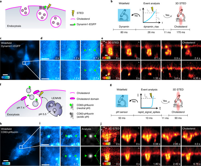
Fig. 3
Investigation of endocytosis and exocytosis with etSTED.
This shows an etSTED experiment in HeLa cells expressing Dynamin1-EGFP or CD63-pHluorin and using the dynamin_rise or rapid_signal_spikes analysis pipeline. a , Schematic diagram of the dynamin-mediat...

Fig. 4
Investigation of endosomal vesicle interaction with etSTED.
This shows an etSTED experiment in hippocampal neurons expressing CD63-EGFP and using the vesicle_proximity analysis pipeline. a , Schematic diagram of an endosomal vesicle interaction process, with t...

Extended Data Fig. 1
Applications of etSTED analysis pipelines.
a , rapid_signal_spikes applied to hippocampal neurons labeled with BAPTA-OregonGreen488 to detect calcium spikes. Representative example from Nu2009=u2009946 events, Nu2009=u200962 cells. b , rapid_s...

Extended Data Fig. 2
Characterization of etSTED: coordinate transform and etSTED experiments with calcium event triggering and STED imaging of microtubules.
a , Characterization of residual shift after coordinate transformation between widefield and scanning space across the field of view (FOV). Nu2009=u20091048 beads. b , etSTED experiment in HeLa cells ...

Extended Data Fig. 3
etSTED experiments in neurons with widefield imaging of calcium signaling (BAPTA-1) and STED timelapse imaging of actin (SiR-actin).
a , Mean widefield image of all triggering widefield frames. b , Maximum-projected analysis ratiometric image of all detected events in experiment. Green squares show location of detected events ( a ,...

Extended Data Fig. 4
etSTED experiment in neurons with calcium imaging (Oregon Green 488 BAPTA-1) and STED timelapse imaging of synaptic vesicles (synaptotagmin-1_STAR635P).
a , Mean image of all widefield frames with detected events. Boxes are centered on the coordinates of true (green) and false (magenta) detected events. b , Maximum projection of all ratiometric prepro...

Extended Data Fig. 5
Manual STED timelapse imaging of synaptic vesicles (synaptotagmin-1_STAR635P).
a , STED timelapses of synaptic vesicle clusters in active synapses. b , Distributions of area (left) and aspect ratio (right) for the clusters in calcium-activity-triggered STED timelapses (red) and ...

Extended Data Fig. 6
Imaging of synaptic vesicle dynamics with etSTED at 23u2009Hz.
a , (left) Oregon Green 488 BAPTA-1 widefield image. ROI I shows the neurite region in which a calcium event was detected. (right) Single frames of a STED timelapse recording showing synaptotagmin-1_S...

Extended Data Fig. 7
etSTED experiments in HeLa cells with widefield imaging of dynamin (dynamin1-EGFP) and 3D STED timelapse imaging of membrane dynamics (cholesterol-KK114) during endocytosis.
a , Widefield images leading up to the triggering frame (last image), showing the slow rise in fluorescence signal signifying recruitment of dynamin at the site. b , Representative frames from 5.9u200...

Extended Data Fig. 8
etSTED experiments in HeLa cells with widefield imaging of CD63-pHluorin and 3D STED timelapse imaging of membrane dynamics (cholesterol-KK114) during exocytosis.
a , Widefield images leading up to the triggering frame (last image), showing the rapidly appearing (frame-to-frame) fluorescence signal signifying a local pH neutralization at the site. b , Represent...

Extended Data Fig. 9
etSTED experiments in HeLa cells with widefield imaging of intracellular vesicles (CD63-EGFP) and STED timelapse imaging of membrane dynamics (cholesterol-KK114) during intracellular vesicle interaction.
a , Widefield images leading up to the triggering frame (last image), showing the increasing proximity of two vesicles (asterisk (mobile) and arrow (stationary)) indicating a potential interaction. b ...
Figure images are served from the NIH/NLM PubMed Central Open Access Subset or Europe PMC; copyright remains with the publishers and authors.
💬 Discussion
0 commentsNo comments yet. Be the first to start a discussion!
Leave a Comment