Abstract
Expansion microscopy (ExM) allows scalable imaging of preserved 3D biological specimens with nanoscale resolution on fast diffraction-limited microscopes. Here, we explore the utility of ExM in the larval and embryonic zebrafish, an important model organism for the study of neuroscience and development. Regarding neuroscience, we found that ExM enabled the tracing of fine processes of radial glia, which are not resolvable with diffraction-limited microscopy. ExM further resolved putative synaptic connections, as well as molecular differences between densely packed synapses. Finally, ExM could resolve subsynaptic protein organization, such as ring-like structures composed of glycine receptors. Regarding development, we used ExM to characterize the shapes of nuclear invaginations and channels, and to visualize cytoskeletal proteins nearby. We detected nuclear invagination channels at late prophase and telophase, potentially suggesting roles for such channels in cell division. Thus, ExM of the larval and embryonic zebrafish may enable systematic studies of how molecular components are configured in multiple contexts of interest to neuroscience and developmental biology.
🔬 Techniques
🔭 Microscopes
🧬 Organisms
✨ Fluorophores
🧪 Sample Preparation
🏭 Microscope Brands
🧪 Reagent Suppliers
💻 Software Details
🏛️ Research Organizations (ROR)
Affiliated research institutions:
📋 Methods
Fish Maintenance and Care. All zebrafish ( Danio rerio ) larvae were raised in fish facility water at Harvard University according to protocols and procedures approved by the Harvard University/Faculty of Arts & Sciences Standing Committee on the Use of Animals in Research and Teaching (Institutional Animal Care and Use Committee), with the following exceptions: Larvae used in Fig. 1 and SI Appendix , Fig. S1 A , B , and D and one of two larvae used for the analysis shown in SI Appendix , Fig. S1 C were raised in Danieau’s medium at the Max Planck Institute of Neurobiology. These animal procedures conformed to the institutional guidelines of the Max Planck Society and the local government (Regierung von Oberbayern). Experimental protocols were approved by Regierung von Oberbayern (55.2-1-54-2532-101-12 and 55.2-1-54-2532-31-2016). All larvae were raised on a standard 14-h light/10-h dark cycle at a temperature of 28 °C. Fig. 1. ExM helps resolve the morphology of fine cellular processes. ( A ) Schematic of the larval zebrafish brain showing the imaged area (red rectangle) within the left optic tectum. ( B and B′ ) Maximum intensity projections of part of the tectum (highlighted in red in A ) of a 6-d postfertilization larval zebrafish sparsely expressing membrane-bound EGFP and stained for GFP preexpansion ( B ) and postexpansion ( B ′), showing radial glial cells (two of which are labeled RG1 and RG2) and projection fiber bundles (arrowheads). ( C and C′ ) Single confocal slices show projections of cell RG1, preexpansion ( C ) and postexpansion ( C ′). Endfeet processes of this cell wrap around the cell body of a superficial interneuron [SIN ( 113 ); arrow]. ( D and D′ ) A bundle of extratectal fibers preexpansion ( D ) and postexpansion ( D ′) from the regions highlighted by arrowheads in B and B ′, respectively, is shown. ( E and E ′) Intensity plots along the orange line in D and D ′, respectively. AU, arbitrary units. [Scale bars: B , 10 μm; B ′, 10 μm (physical size postexpansion, 35 μm); C and D , 5 μm; C ′ and D ′, 5 μm (17.5 μm).] Transgenic Fish Lines. The genotypes of the larvae and embryos used to generate each figure are detailed in SI Appendix , SI Methods . The transgenic fish lines that were crossed to produce these larvae and embryos were all previously described. All larval brain images are from 6-d postfertilization larvae, and all embryo images are from shield-stage (i.e., ∼6-h postfertilization) embryos. Immunohistochemistry. Immunohistochemistry was performed following standard, previously published procedures ( 28 ). The exact protocol, as well as a detailed list of antibodies used, is provided in SI Appendix , SI Methods . Expansion. Expansion was performed using the previously described proExM protocol ( 2 ) ( SI Appendix , SI Methods ). Imaging. Both pre- and postexpansion brains and embryos were imaged on an Andor spinning disk (CSU-X1 Yokogawa) confocal system with a 40×, 1.15 N.A. water immersion objective (Nikon), with the exception of some images in SI Appendix , Fig. S1 : The first and third images in SI Appendix , Fig. S1 A and all preexpansion images used to generate SI Appendix , Fig. S1 C were acquired using a Deltavision OMX Blaze (GE Healthcare) structured-illumination microscope (SIM) with a 60×, 1.42 N.A. oil immersion objective (Olympus). These brains were immersed in SlowFade Diamond Antifade mounting medium (Invitrogen) for refractive index matching and suppression of bleaching. The first and third images in SI Appendix , Fig. S1 B and all preexpansion images used to generate SI Appendix , Fig. S1 D were acquired using a Leica TCS SP8 STED microscope, with a 100×, 1.4 N.A. oil immersion objective. These brains were immersed in SlowFade Gold Antifade mounting medium (Invitrogen) for refractive index matching and suppression of bleaching. The second and fourth images in SI Appendix , Fig. S1 B and all postexpansion images used to generate SI Appendix , Fig. S1 D were acquired using a Leica TCS SP8 confocal microscope, with a 40×, 1.1 N.A. water immersion objective. Images of the samples were also obtained with a 10×, 0.45 N.A. air objective and used to aid in the comparison of pre- and postexpansion data and computation of expansion factors. Details of excitation and emission collection are provided in SI Appendix , SI Methods . For embryos, postexpansion imaging was also performed via a Nikon Ti-E epifluorescence microscope with a 4×, 0.13 N.A. air objective to allow capturing of the entire sample for computation of expansion factors. For brains, expansion factors were computed by measuring the size of specific anatomical features (e.g., the axon cap) pre- vs. postexpansion, and taking the ratio of the respective sizes. For embryos, the diameter of the embryo pre- vs. postexpansion was compared. Scale bars on postexpansion images reflect these expansion factor computations. For the expanded embryos imaged in SI Appendix , Fig. S10 , pre- and postexpansion images were taken from very different angles; thus, an exact expansion factor could not be computed. For SI Appendix , Fig. S10 , an expansion factor of 4 [similar to the expansion factors computed for other embryos (3.8 and 4.1)] was estimated for the purpose of drawing scale bars. Image Processing. Each figure panel constitutes a single plane from a z-stack, where the area of interest was cropped out of the field of view using Fiji ( 29 ), or a maximal intensity projection, as indicated in the figure legends. The brightness and contrast of individual channels were adjusted in ImageJ (NIH) after cropping the area of interest. The STED preexpansion images shown in SI Appendix , Fig. S1 B (first and third panels) and used in SI Appendix , Fig. S1 D were deconvolved using Huygens (Scientific Volume Imaging). Tracing of cellular processes (shown in SI Appendix , Fig. S2 ) was performed using Imaris. This tracing algorithm is intensity-based. First, start and end points are detected, and then these points are connected with traces following the image intensity. Fig. 2 B is a maximal intensity projection of four stacks acquired separately and stitched together using Fiji’s pairwise stitching plug-in ( 30 ). The data shown in Fig. 3 B – E and SI Appendix , Figs. S5 and S6 were cropped from stacks following illumination correction using CIDRE ( 31 ) and deconvolution using Huygens. Since the illumination model is dictated by the microscope optics, a single illumination model was learned using CIDRE by pooling the datasets together, and then this same model was used for the correction of both pre- and postexpansion datasets. After the application of illumination correction, a dataset-specific threshold was manually set according to the characteristic background noise level. Both pre- and postexpansion datasets were then deconvolved using the exact same procedure and parameters. Fig. 2. ExM analysis of synaptic connections. ( A ) Schematic of larval zebrafish brain showing nIII and nIV nuclei, labeled by Tg(isl1:GFP)rw0 (GFP, yellow) and neural projections labeled by Tg(−6.7FRhcrtR:Gal4VP16);Tg(UAS:Kaede) (Kaede, magenta). The rectangular area is imaged in B . ( B ) Maximal intensity projection of an ∼33-μm-thick volume corresponding to the rectangular area shown in A . The fish is 6 d postfertilization (dpf), and is stained with anti-GFP (yellow), anti-Kaede (magenta), and anti–pan-MAGUK (not shown). ( C ) GFP-labeled cells (yellow) and Kaede-labeled projections (magenta) in the nIII nucleus. ( C , I – IV and I ′– IV ′) Two nearby planes (one in each row) from an expanded 6-dpf brain stained with anti-GFP (yellow), anti-Kaede (magenta), and anti-synaptotagmin2b (cyan). Arrows point to Kaede-expressing and synaptotagmin2b-stained varicosities and terminals next to GFP-labeled neuropil ( IV ) and cell bodies ( IV ′). Arrowheads point to a cluster of synaptotagmin2b, unlabeled by Kaede, next to a GFP-labeled cell ( IV ) and a Kaede-labeled synaptotagmin2b-stained varicosity next to a GFP-negative cell ( IV ′). ( C , V – VIII ) Single plane from a brain stained with anti–pan-MAGUK (cyan). Arrows point to Kaede-labeled varicosities and terminals next to GFP-labeled cells and neuropil, exhibiting colocalized MAGUK puncta. Arrowheads point to a MAGUK punctum on a GFP-negative cell opposed to a Kaede-labeled terminal ( Top arrowhead) and to MAGUK puncta on GFP-labeled cell bodies and neuropil in the absence of nearby Kaede-labeled projections ( Bottom two arrowheads). [Scale bars: B , 10 μm (38 μm); C , I – IV and I ′– IV ′, 5 μm (23 μm); C , V – VIII , 5 μm (19 μm).] Fig. 3. Expansion enables the resolving of synaptic heterogeneity and structure in intrasynaptic protein distributions. ( A ) Schematic of a larval zebrafish brain showing the M cells (blue) and spiral fiber neurons (magenta). The rectangle illustrates the region focused in on in B – D , consisting of the axon cap and a part of the M cell body. ( B ) Preexpansion images of the axon-cap area showing spiral fiber neurons (magenta) wrapping around the M cell axon initial segment (the unlabeled “tube” passing through these fibers, better visualized as a black stripe in C ), as well as synaptotagmin2b ( Top , cyan) and glycine receptors ( Bottom , cyan). ( C ) Same as in B , but postexpansion. (Note: The synaptotagmin2b axon cap shown ( Top ) is not from the same brain as in B, Top .) ( Top Left and Right ) Arrows point to a Kaede-labeled varicosity bearing synaptotagmin2b at a low density. ( Top Left and Right ) Arrowheads point to a Kaede-negative varicosity bearing dense synaptotagmin2b staining. ( Center ) Arrowheads point to varicosities in spiral fiber neuron projections forming the M cell axon cap. ( D ) Maximal intensity projection of the M cell body and axon initial segment area showing the distribution of glycine receptors (cyan) preexpansion ( Left ) vs. postexpansion ( Right ). (Note: This is the same axon cap as shown in B and C, Bottom .) Boxes highlight seven examples of ring-shaped clusters zoomed in on in E . ( E ) Seven examples of ring-shaped clusters of various sizes present on the M cell body (1–6), and axon (7). [Scale bars: B , Top and Bottom, 5 μm; C , Top , 5 μm (23 μm); C , Bottom , 5 μm (20 μm); D , Left , 5 μm; D , Right , 5 μm (20 μm); E , 1 μm (4 μm).] Measurement Error Quantification. Errors were quantified using the same procedures as previously described ( 2 , 32 ), with a few exceptions ( SI Appendix , SI Methods ).
Show full methods section
Fish Maintenance and Care. All zebrafish ( Danio rerio ) larvae were raised in fish facility water at Harvard University according to protocols and procedures approved by the Harvard University/Faculty of Arts & Sciences Standing Committee on the Use of Animals in Research and Teaching (Institutional Animal Care and Use Committee), with the following exceptions: Larvae used in Fig. 1 and SI Appendix , Fig. S1 A , B , and D and one of two larvae used for the analysis shown in SI Appendix , Fig. S1 C were raised in Danieau’s medium at the Max Planck Institute of Neurobiology. These animal procedures conformed to the institutional guidelines of the Max Planck Society and the local government (Regierung von Oberbayern). Experimental protocols were approved by Regierung von Oberbayern (55.2-1-54-2532-101-12 and 55.2-1-54-2532-31-2016). All larvae were raised on a standard 14-h light/10-h dark cycle at a temperature of 28 °C. Fig. 1. ExM helps resolve the morphology of fine cellular processes. ( A ) Schematic of the larval zebrafish brain showing the imaged area (red rectangle) within the left optic tectum. ( B and B′ ) Maximum intensity projections of part of the tectum (highlighted in red in A ) of a 6-d postfertilization larval zebrafish sparsely expressing membrane-bound EGFP and stained for GFP preexpansion ( B ) and postexpansion ( B ′), showing radial glial cells (two of which are labeled RG1 and RG2) and projection fiber bundles (arrowheads). ( C and C′ ) Single confocal slices show projections of cell RG1, preexpansion ( C ) and postexpansion ( C ′). Endfeet processes of this cell wrap around the cell body of a superficial interneuron [SIN ( 113 ); arrow]. ( D and D′ ) A bundle of extratectal fibers preexpansion ( D ) and postexpansion ( D ′) from the regions highlighted by arrowheads in B and B ′, respectively, is shown. ( E and E ′) Intensity plots along the orange line in D and D ′, respectively. AU, arbitrary units. [Scale bars: B , 10 μm; B ′, 10 μm (physical size postexpansion, 35 μm); C and D , 5 μm; C ′ and D ′, 5 μm (17.5 μm).] Transgenic Fish Lines. The genotypes of the larvae and embryos used to generate each figure are detailed in SI Appendix , SI Methods . The transgenic fish lines that were crossed to produce these larvae and embryos were all previously described. All larval brain images are from 6-d postfertilization larvae, and all embryo images are from shield-stage (i.e., ∼6-h postfertilization) embryos. Immunohistochemistry. Immunohistochemistry was performed following standard, previously published procedures ( 28 ). The exact protocol, as well as a detailed list of antibodies used, is provided in SI Appendix , SI Methods . Expansion. Expansion was performed using the previously described proExM protocol ( 2 ) ( SI Appendix , SI Methods ). Imaging. Both pre- and postexpansion brains and embryos were imaged on an Andor spinning disk (CSU-X1 Yokogawa) confocal system with a 40×, 1.15 N.A. water immersion objective (Nikon), with the exception of some images in SI Appendix , Fig. S1 : The first and third images in SI Appendix , Fig. S1 A and all preexpansion images used to generate SI Appendix , Fig. S1 C were acquired using a Deltavision OMX Blaze (GE Healthcare) structured-illumination microscope (SIM) with a 60×, 1.42 N.A. oil immersion objective (Olympus). These brains were immersed in SlowFade Diamond Antifade mounting medium (Invitrogen) for refractive index matching and suppression of bleaching. The first and third images in SI Appendix , Fig. S1 B and all preexpansion images used to generate SI Appendix , Fig. S1 D were acquired using a Leica TCS SP8 STED microscope, with a 100×, 1.4 N.A. oil immersion objective. These brains were immersed in SlowFade Gold Antifade mounting medium (Invitrogen) for refractive index matching and suppression of bleaching. The second and fourth images in SI Appendix , Fig. S1 B and all postexpansion images used to generate SI Appendix , Fig. S1 D were acquired using a Leica TCS SP8 confocal microscope, with a 40×, 1.1 N.A. water immersion objective. Images of the samples were also obtained with a 10×, 0.45 N.A. air objective and used to aid in the comparison of pre- and postexpansion data and computation of expansion factors. Details of excitation and emission collection are provided in SI Appendix , SI Methods . For embryos, postexpansion imaging was also performed via a Nikon Ti-E epifluorescence microscope with a 4×, 0.13 N.A. air objective to allow capturing of the entire sample for computation of expansion factors. For brains, expansion factors were computed by measuring the size of specific anatomical features (e.g., the axon cap) pre- vs. postexpansion, and taking the ratio of the respective sizes. For embryos, the diameter of the embryo pre- vs. postexpansion was compared. Scale bars on postexpansion images reflect these expansion factor computations. For the expanded embryos imaged in SI Appendix , Fig. S10 , pre- and postexpansion images were taken from very different angles; thus, an exact expansion factor could not be computed. For SI Appendix , Fig. S10 , an expansion factor of 4 [similar to the expansion factors computed for other embryos (3.8 and 4.1)] was estimated for the purpose of drawing scale bars. Image Processing. Each figure panel constitutes a single plane from a z-stack, where the area of interest was cropped out of the field of view using Fiji ( 29 ), or a maximal intensity projection, as indicated in the figure legends. The brightness and contrast of individual channels were adjusted in ImageJ (NIH) after cropping the area of interest. The STED preexpansion images shown in SI Appendix , Fig. S1 B (first and third panels) and used in SI Appendix , Fig. S1 D were deconvolved using Huygens (Scientific Volume Imaging). Tracing of cellular processes (shown in SI Appendix , Fig. S2 ) was performed using Imaris. This tracing algorithm is intensity-based. First, start and end points are detected, and then these points are connected with traces following the image intensity. Fig. 2 B is a maximal intensity projection of four stacks acquired separately and stitched together using Fiji’s pairwise stitching plug-in ( 30 ). The data shown in Fig. 3 B – E and SI Appendix , Figs. S5 and S6 were cropped from stacks following illumination correction using CIDRE ( 31 ) and deconvolution using Huygens. Since the illumination model is dictated by the microscope optics, a single illumination model was learned using CIDRE by pooling the datasets together, and then this same model was used for the correction of both pre- and postexpansion datasets. After the application of illumination correction, a dataset-specific threshold was manually set according to the characteristic background noise level. Both pre- and postexpansion datasets were then deconvolved using the exact same procedure and parameters. Fig. 2. ExM analysis of synaptic connections. ( A ) Schematic of larval zebrafish brain showing nIII and nIV nuclei, labeled by Tg(isl1:GFP)rw0 (GFP, yellow) and neural projections labeled by Tg(−6.7FRhcrtR:Gal4VP16);Tg(UAS:Kaede) (Kaede, magenta). The rectangular area is imaged in B . ( B ) Maximal intensity projection of an ∼33-μm-thick volume corresponding to the rectangular area shown in A . The fish is 6 d postfertilization (dpf), and is stained with anti-GFP (yellow), anti-Kaede (magenta), and anti–pan-MAGUK (not shown). ( C ) GFP-labeled cells (yellow) and Kaede-labeled projections (magenta) in the nIII nucleus. ( C , I – IV and I ′– IV ′) Two nearby planes (one in each row) from an expanded 6-dpf brain stained with anti-GFP (yellow), anti-Kaede (magenta), and anti-synaptotagmin2b (cyan). Arrows point to Kaede-expressing and synaptotagmin2b-stained varicosities and terminals next to GFP-labeled neuropil ( IV ) and cell bodies ( IV ′). Arrowheads point to a cluster of synaptotagmin2b, unlabeled by Kaede, next to a GFP-labeled cell ( IV ) and a Kaede-labeled synaptotagmin2b-stained varicosity next to a GFP-negative cell ( IV ′). ( C , V – VIII ) Single plane from a brain stained with anti–pan-MAGUK (cyan). Arrows point to Kaede-labeled varicosities and terminals next to GFP-labeled cells and neuropil, exhibiting colocalized MAGUK puncta. Arrowheads point to a MAGUK punctum on a GFP-negative cell opposed to a Kaede-labeled terminal ( Top arrowhead) and to MAGUK puncta on GFP-labeled cell bodies and neuropil in the absence of nearby Kaede-labeled projections ( Bottom two arrowheads). [Scale bars: B , 10 μm (38 μm); C , I – IV and I ′– IV ′, 5 μm (23 μm); C , V – VIII , 5 μm (19 μm).] Fig. 3. Expansion enables the resolving of synaptic heterogeneity and structure in intrasynaptic protein distributions. ( A ) Schematic of a larval zebrafish brain showing the M cells (blue) and spiral fiber neurons (magenta). The rectangle illustrates the region focused in on in B – D , consisting of the axon cap and a part of the M cell body. ( B ) Preexpansion images of the axon-cap area showing spiral fiber neurons (magenta) wrapping around the M cell axon initial segment (the unlabeled “tube” passing through these fibers, better visualized as a black stripe in C ), as well as synaptotagmin2b ( Top , cyan) and glycine receptors ( Bottom , cyan). ( C ) Same as in B , but postexpansion. (Note: The synaptotagmin2b axon cap shown ( Top ) is not from the same brain as in B, Top .) ( Top Left and Right ) Arrows point to a Kaede-labeled varicosity bearing synaptotagmin2b at a low density. ( Top Left and Right ) Arrowheads point to a Kaede-negative varicosity bearing dense synaptotagmin2b staining. ( Center ) Arrowheads point to varicosities in spiral fiber neuron projections forming the M cell axon cap. ( D ) Maximal intensity projection of the M cell body and axon initial segment area showing the distribution of glycine receptors (cyan) preexpansion ( Left ) vs. postexpansion ( Right ). (Note: This is the same axon cap as shown in B and C, Bottom .) Boxes highlight seven examples of ring-shaped clusters zoomed in on in E . ( E ) Seven examples of ring-shaped clusters of various sizes present on the M cell body (1–6), and axon (7). [Scale bars: B , Top and Bottom, 5 μm; C , Top , 5 μm (23 μm); C , Bottom , 5 μm (20 μm); D , Left , 5 μm; D , Right , 5 μm (20 μm); E , 1 μm (4 μm).] Measurement Error Quantification. Errors were quantified using the same procedures as previously described ( 2 , 32 ), with a few exceptions ( SI Appendix , SI Methods ).
Supplementary Material Supplementary File Supplementary File Supplementary File Supplementary File Supplementary File Supplementary File Supplementary File Supplementary File Supplementary File Supplementary File Supplementary File Supplementary File Supplementary File
📊 Figures
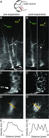
Fig. 1.
ExM helps resolve the morphology of fine cellular processes. ( A ) Schematic of the larval zebrafish brain showing the imaged area (red rectangle) within the left optic tectum. ( B and Bu2032 ) Maximu...
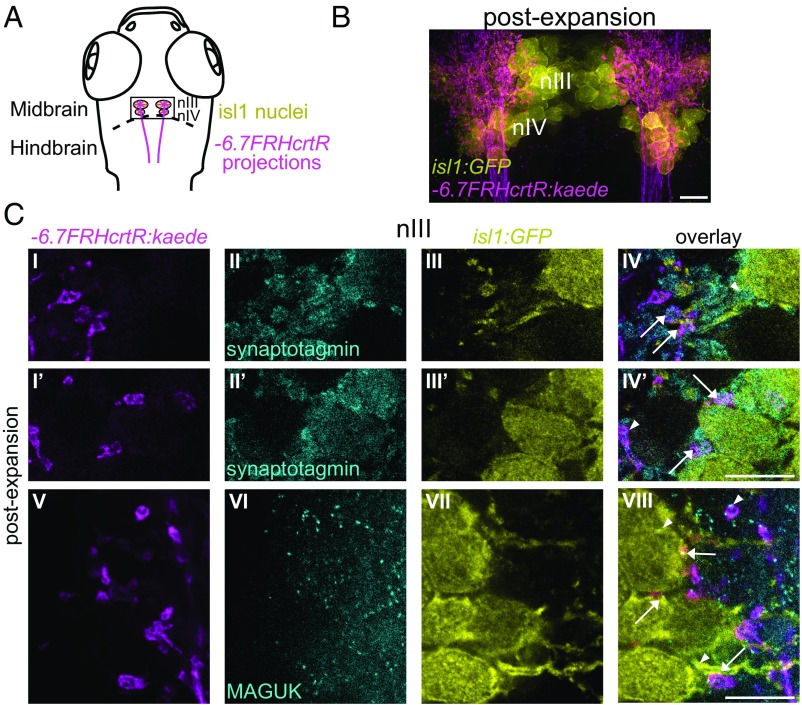
Fig. 2.
ExM analysis of synaptic connections. ( A ) Schematic of larval zebrafish brain showing nIII and nIV nuclei, labeled by Tg(isl1:GFP)rw0 (GFP, yellow) and neural projections labeled by Tg(u22126.7FRhcr...
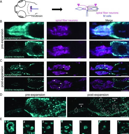
Fig. 3.
Expansion enables the resolving of synaptic heterogeneity and structure in intrasynaptic protein distributions. ( A ) Schematic of a larval zebrafish brain showing the M cells (blue) and spiral fiber ...
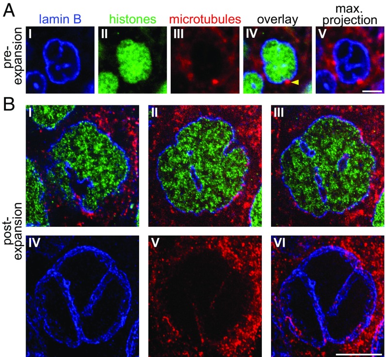
Fig. 4.
ExM examination of intranuclear invaginations. In all panels in this figure, in Figs. 5 and 6 , and in Movies S5u2013S8 : blue, anti-lamin B; green, histone 2B [EGFP fused to histone 2B in Tg(actb2:h2...
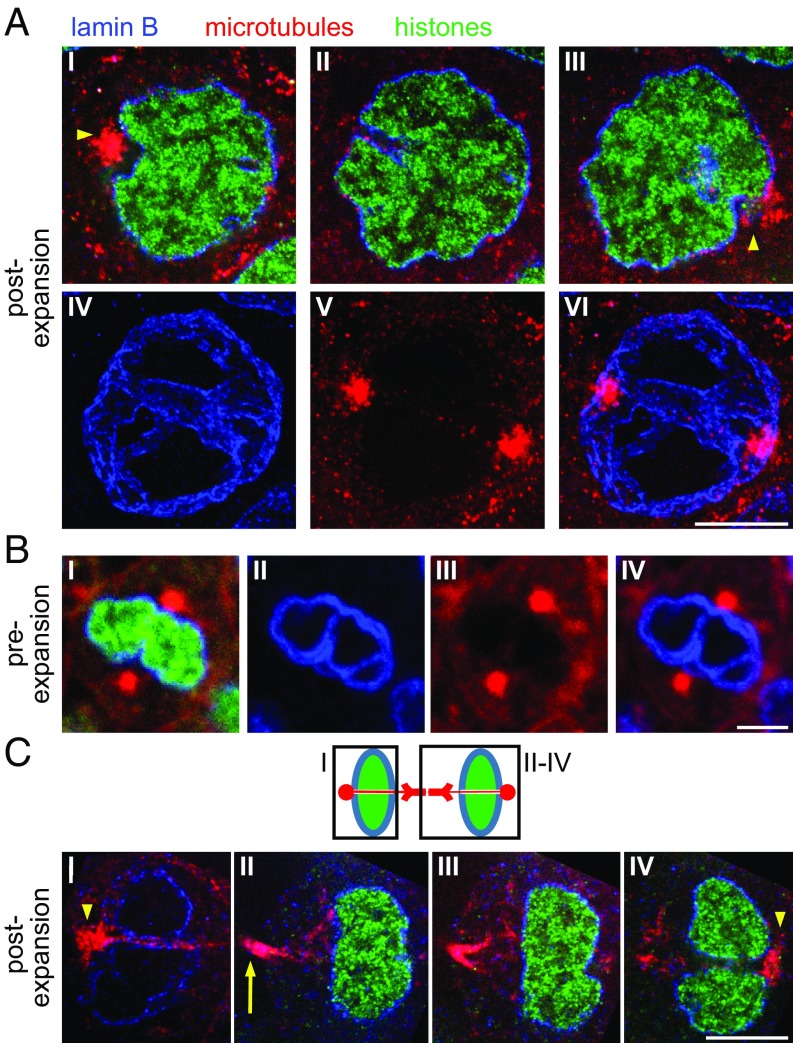
Fig. 5.
ExM reveals intranuclear channels in late-prophase and telophase nuclei. ( A ) Nucleus at late prophase, postexpansion. ( A , I u2013 III ) Three planes from the nucleus. ( A , I ) Arrowhead points to...
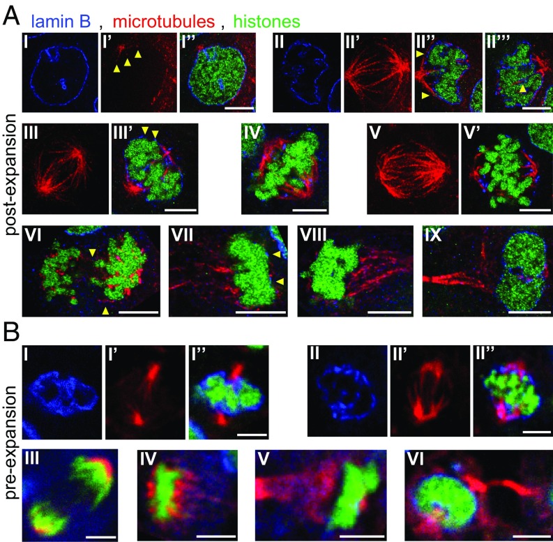
Fig. 6.
ExM and the analysis of mitotic nuclei. ( A ) Mitotic nuclei, postexpansion. ( A , I u2013 I u2032u2032) Nucleus at the transition between prophase and prometaphase. ( A , I ) Lamin B staining. ( A , ...
Figure images are served from the NIH/NLM PubMed Central Open Access Subset or Europe PMC; copyright remains with the publishers and authors.
💬 Discussion
0 commentsNo comments yet. Be the first to start a discussion!
Leave a Comment