Abstract
MINFLUX offers a breakthrough in single molecule localization precision, but is limited in field of view. Here we combine centroid estimation and illumination pattern induced photon count variations in a conventional widefield imaging setup to extract position information over a typical micrometer-sized field of view. We show a near two-fold improvement in precision over standard localization with the same photon count on DNA-origami nanostructures and tubulin in cells, using DNA-PAINT and STORM imaging.
🔬 Techniques
🔭 Microscopes
💻 Software
✨ Fluorophores
🧪 Sample Preparation
🔬 Cell Lines
🏭 Microscope Brands
🧪 Reagent Suppliers
📷 Detectors
🎨 Filters
💻 Software Details
💻 Code & Software
💾 Data Repositories
🏛️ Research Organizations (ROR)
Affiliated research institutions:
📋 Methods
Experimental setup
A custom total internal reflection (TIRF) structured illumination microscopy (SIM) microscope was built to implement the SIMFLUX method ( Supplementary Figure 14 ). The setup uses a 200 mW, 640 nm, diode laser (Toptica, CLUP-640) that is spectrally filtered with a 640/20 nm (Chroma, ET640/20m) bandpass filter and spatially filtered by coupling into a polarization maintaining single mode fiber (ThorLabs, PM630-HP) via an NA matched aspheric lens, L1 (f = 3.3 mm, ThorLabs, C340TMD-A). The output of the fiber is collimated by an objective, L2 (0.45/20X A-PLAN, Zeiss). SIMFLUX utilizes two orthogonal sinusoidal modulation patterns in the focal plane of the objective lens. The optical architecture overcomes drawbacks of typical SIM architectures. Rotating gratings are too slow to generate multiple illumination patterns for a typical molecular on-event (~10s of ms), Spatial Light Modulators (SLMs) are sufficiently fast, but too power-inefficient to generate a sufficiently high illumination intensity (~kW/cm 2 ) over an extended field of view (~10s of μm). A simple way to generate these is to build an interferometer and self-interfere a laser at the sample plane. The approach is a modification of an earlier architecture, where two pairs of diffraction orders are generated with two orthogonally oriented gratings and combined with a polarizing beam splitter 21 . In our setup, custom etched binary phase gratings (HOLOOR, DS-28101-Y-A) with pitches of 8.496 μm are used to generate ±1st diffraction orders with near theoretical diffraction efficiency limits of around 79%. Distinct and orthogonal interference patterns at the focal plane with controllable phase are generated using a fluid filled KD*P Pockels cell (Leysop, EM508-2T-F-AR640) to alternate the laser between two beam paths and piezoelectric stages (PI, P-753.1CD) to phase shift the binary phase gratings. Before being sent through the Pockels cell and diffraction gratings, the laser intensity is controlled via a half wave plate (ThorLabs, DS-281-1-Y-A) and a Glan-Taylor polarizer (GL10-A) to attenuate when needed while maintaining at least a 1000:1 intensity extinction ratio between each path. The beam then passes through the Pockels cell that is aligned such that applying a half wave voltage switches the beam between s and p polarizations. Two mirrors (ThorLabs, PF10-03-G01) then align the laser to the main optical axis of the system. A quarter wave plate and half wave plate (ThorLabs, WPQ05M-633 & WPH05M-633) are placed after the second mirror to reduce any elliptical polarization induced by reflection. A cube polarizing beam splitter (ThorLabs, CCM1-PBS252/M) selects the beam path based on s or p polarization entry. A high extinction ratio Glan-Taylor polarizer (ThorLabs, GL10-A) is then placed in each beam path after the polarizing beam splitter to ensure at least 10 4 polarization purity in each beam path. A binary phase grating is then placed in both beam paths. Each grating is mounted on a nanometer resolution piezoelectric translation stage to induce phase shifting. The stages have a step and settle time of 3–4 ms, giving an upper limit to the framerate of 250 Hz. The gratings are aligned on the piezoelectric stages so that their main diffraction axes are orthogonal to one another. The azimuthal alignment of the gratings is chosen such that the polarization of the interfering diffraction orders is parallel in the objective focal plane for each beam path. After light is diffracted from each binary phase grating, a second polarizing beam splitter recombines the two paths into the main system illumination path. Two more beam steering mirrors are needed to recombine the beam path that is reflected off the first beam splitter. After recombining into a single optical axis, the diffracted orders are collimated by L3 (ThorLabs, ACA254-075-A) and sent through a spatial filter mask to filter all but the ±1st diffraction orders. From there a 4f system L4,5 (Edmund Optics/ThorLabs, 49-395-INK/AC508-180-A-ML) relays the spatial filter to the rear focal plane of the objective (Nikon, CFI Apo 1.49 TIRF 100XC Oil) after reflecting off a long pass dichroic mirror (Semrock, Di03-R660-t1-25.2×35.6). If the light from the ±1st orders is well focused in the rear focal plane, collimated light will emerge from the objective and be incident on the sample plane. Careful alignment is needed here, as a defocus at the rear focal plane will result in a distortion of the sinusoidal illumination pattern. The ±1st orders enter at opposite edges of the back focal plane at a radius ±2.91 mm from the optical axis, corresponding to a Numerical Aperture NA i = 2.9½.0 = 1.455 (the focal length of the Nikon 100x objective lens is 2.0 mm). The illumination NA i exceeds the sample refractive index of n med = 1.33 and therefore provides TIRF illumination. A TIRF illumination system is chosen in order to reduce background fluorescence by providing an interface bound optical sectioning of 100–200 nm, and to be compatible with DNA-PAINT based localization. The sample plane is illuminated with a power density of ~600 W/cm 2 over an 80 μm illumination diameter. Control of the sample plane and system focus is achieved with a XYZ 100×100×100 μm travel range piezoelectric slide stage (Mad City Labs, 1D100). Emitted fluorescence is collected by the same Nikon objective in an epi-illumination configuration and passes through the long pass dichroic mirror and a bandpass 690/50 nm emission filter (Chroma, ET690/50m) before being imaged by an infinity corrected tube lens (ThorLabs, TTL200-A) onto an sCMOS camera (Hamamatsu, ORCA Flash 4.0 V2). The pixel size of our camera in the sensor plane is 6.5 μm giving a back-projected pixel size in the sample plane equal to 65 nm. Image acquisition was controlled using a standard desktop workstation equipped with a camera link frame grabber (Hamamatsu, AS-FBD-1XCLD-2PE8). Micro-manager serves as the main image acquisition software, but is integrated with a custom Python script to control an Arduino which triggers the PI piezoelectric stage controllers and the Pockels cell to iterate through imaging states. Micro-manager also controls the piezoelectric sample stage from Mad City Labs. The PI piezo electric stages were initialized to receive triggers from the Arduino via the program MikroMove. A second set of hardware was incorporated into the system to facilitate (d)STORM imaging. These alterations included replacing the original sCMOS (Hamamatsu, ORCA Flash 4.0 V2) with another sCMOS (Andor, Zyla 4.2) for better pixel blanking between subsequent frames. The laser was replaced with a 200 mW, 638 nm, laser diode (Omicron, PhoxX+ 638–200) in a fiber-less free space configuration to achieve an appropriate power density at the sample plane of ~1.5 kW/cm 2 for (d)STORM imaging. Micro-manager was also replaced with the Andor Solis frame capture software to facilitate high speed spooling to hard disk without data loss. The modulation contrast of the system was characterized by imaging a pre-prepared slide of 20 nm GATTA-beads (GattaQuant, Bead R) and finely phase shifting the illumination pattern over the sample. By imaging after each phase shift, a direct measurement of the sinusoidal wave can be traced over the image series duration ( Supplementary Figure 15 ). Median values of the modulation contrast of 0.91 and 0.92 in the two pattern directions were measured. The observed values for the modulation contrast may be related to polarization impurity at the back focal plane. An analysis of the electromagnetic evanescent wave at the sample results in a modulation contrast m ≈ 1 − 2( NA i 2 / n med 2 ) R , with R the intensity ratio of undesired (p) to desired (s) polarization at the back focal plane. Excluding other causes, a value of R around 3 to 4% is consistent with the observed modulation contrast. A contributing factor to polarization impurity could be the reflection of the beams converging to the back focal plane of the objective after reflection at the dichroic. The polarization purity may also be affected by the quality of the dichroic. According to the specification of the manufacturer, the reflection for s-polarized light is at near 100%, and the reflection for p-polarized light is about 98%, at the laser wavelength of 640 nm. The pitch of the interference pattern in the sample plane was calibrated by imaging high density, blinking, fluorophores that are evenly distributed in the sample plane, and localizing the fluorophores under static standing wave illumination conditions. The illumination pattern arises from the interference of evanescent waves and is therefore not directly visible, however, super-resolved localization images show it quite clearly ( Supplementary Figure 16 ), giving a pitch equal to 219.94 nm. This estimate of the pitch agrees well with the expected value λ ex /(2 NA i ) = 640/(2 * 1.455) = 219.9 nm. The direct calibration of stage translation to phase for the piezo mounted diffraction gratings can be calculated from this data as well, giving a sample plane pattern shift to grating translation ratio of 51.6 nm/μm.
Show full methods section
Experimental setup
A custom total internal reflection (TIRF) structured illumination microscopy (SIM) microscope was built to implement the SIMFLUX method ( Supplementary Figure 14 ). The setup uses a 200 mW, 640 nm, diode laser (Toptica, CLUP-640) that is spectrally filtered with a 640/20 nm (Chroma, ET640/20m) bandpass filter and spatially filtered by coupling into a polarization maintaining single mode fiber (ThorLabs, PM630-HP) via an NA matched aspheric lens, L1 (f = 3.3 mm, ThorLabs, C340TMD-A). The output of the fiber is collimated by an objective, L2 (0.45/20X A-PLAN, Zeiss). SIMFLUX utilizes two orthogonal sinusoidal modulation patterns in the focal plane of the objective lens. The optical architecture overcomes drawbacks of typical SIM architectures. Rotating gratings are too slow to generate multiple illumination patterns for a typical molecular on-event (~10s of ms), Spatial Light Modulators (SLMs) are sufficiently fast, but too power-inefficient to generate a sufficiently high illumination intensity (~kW/cm 2 ) over an extended field of view (~10s of μm). A simple way to generate these is to build an interferometer and self-interfere a laser at the sample plane. The approach is a modification of an earlier architecture, where two pairs of diffraction orders are generated with two orthogonally oriented gratings and combined with a polarizing beam splitter 21 . In our setup, custom etched binary phase gratings (HOLOOR, DS-28101-Y-A) with pitches of 8.496 μm are used to generate ±1st diffraction orders with near theoretical diffraction efficiency limits of around 79%. Distinct and orthogonal interference patterns at the focal plane with controllable phase are generated using a fluid filled KD*P Pockels cell (Leysop, EM508-2T-F-AR640) to alternate the laser between two beam paths and piezoelectric stages (PI, P-753.1CD) to phase shift the binary phase gratings. Before being sent through the Pockels cell and diffraction gratings, the laser intensity is controlled via a half wave plate (ThorLabs, DS-281-1-Y-A) and a Glan-Taylor polarizer (GL10-A) to attenuate when needed while maintaining at least a 1000:1 intensity extinction ratio between each path. The beam then passes through the Pockels cell that is aligned such that applying a half wave voltage switches the beam between s and p polarizations. Two mirrors (ThorLabs, PF10-03-G01) then align the laser to the main optical axis of the system. A quarter wave plate and half wave plate (ThorLabs, WPQ05M-633 & WPH05M-633) are placed after the second mirror to reduce any elliptical polarization induced by reflection. A cube polarizing beam splitter (ThorLabs, CCM1-PBS252/M) selects the beam path based on s or p polarization entry. A high extinction ratio Glan-Taylor polarizer (ThorLabs, GL10-A) is then placed in each beam path after the polarizing beam splitter to ensure at least 10 4 polarization purity in each beam path. A binary phase grating is then placed in both beam paths. Each grating is mounted on a nanometer resolution piezoelectric translation stage to induce phase shifting. The stages have a step and settle time of 3–4 ms, giving an upper limit to the framerate of 250 Hz. The gratings are aligned on the piezoelectric stages so that their main diffraction axes are orthogonal to one another. The azimuthal alignment of the gratings is chosen such that the polarization of the interfering diffraction orders is parallel in the objective focal plane for each beam path. After light is diffracted from each binary phase grating, a second polarizing beam splitter recombines the two paths into the main system illumination path. Two more beam steering mirrors are needed to recombine the beam path that is reflected off the first beam splitter. After recombining into a single optical axis, the diffracted orders are collimated by L3 (ThorLabs, ACA254-075-A) and sent through a spatial filter mask to filter all but the ±1st diffraction orders. From there a 4f system L4,5 (Edmund Optics/ThorLabs, 49-395-INK/AC508-180-A-ML) relays the spatial filter to the rear focal plane of the objective (Nikon, CFI Apo 1.49 TIRF 100XC Oil) after reflecting off a long pass dichroic mirror (Semrock, Di03-R660-t1-25.2×35.6). If the light from the ±1st orders is well focused in the rear focal plane, collimated light will emerge from the objective and be incident on the sample plane. Careful alignment is needed here, as a defocus at the rear focal plane will result in a distortion of the sinusoidal illumination pattern. The ±1st orders enter at opposite edges of the back focal plane at a radius ±2.91 mm from the optical axis, corresponding to a Numerical Aperture NA i = 2.9½.0 = 1.455 (the focal length of the Nikon 100x objective lens is 2.0 mm). The illumination NA i exceeds the sample refractive index of n med = 1.33 and therefore provides TIRF illumination. A TIRF illumination system is chosen in order to reduce background fluorescence by providing an interface bound optical sectioning of 100–200 nm, and to be compatible with DNA-PAINT based localization. The sample plane is illuminated with a power density of ~600 W/cm 2 over an 80 μm illumination diameter. Control of the sample plane and system focus is achieved with a XYZ 100×100×100 μm travel range piezoelectric slide stage (Mad City Labs, 1D100). Emitted fluorescence is collected by the same Nikon objective in an epi-illumination configuration and passes through the long pass dichroic mirror and a bandpass 690/50 nm emission filter (Chroma, ET690/50m) before being imaged by an infinity corrected tube lens (ThorLabs, TTL200-A) onto an sCMOS camera (Hamamatsu, ORCA Flash 4.0 V2). The pixel size of our camera in the sensor plane is 6.5 μm giving a back-projected pixel size in the sample plane equal to 65 nm. Image acquisition was controlled using a standard desktop workstation equipped with a camera link frame grabber (Hamamatsu, AS-FBD-1XCLD-2PE8). Micro-manager serves as the main image acquisition software, but is integrated with a custom Python script to control an Arduino which triggers the PI piezoelectric stage controllers and the Pockels cell to iterate through imaging states. Micro-manager also controls the piezoelectric sample stage from Mad City Labs. The PI piezo electric stages were initialized to receive triggers from the Arduino via the program MikroMove. A second set of hardware was incorporated into the system to facilitate (d)STORM imaging. These alterations included replacing the original sCMOS (Hamamatsu, ORCA Flash 4.0 V2) with another sCMOS (Andor, Zyla 4.2) for better pixel blanking between subsequent frames. The laser was replaced with a 200 mW, 638 nm, laser diode (Omicron, PhoxX+ 638–200) in a fiber-less free space configuration to achieve an appropriate power density at the sample plane of ~1.5 kW/cm 2 for (d)STORM imaging. Micro-manager was also replaced with the Andor Solis frame capture software to facilitate high speed spooling to hard disk without data loss. The modulation contrast of the system was characterized by imaging a pre-prepared slide of 20 nm GATTA-beads (GattaQuant, Bead R) and finely phase shifting the illumination pattern over the sample. By imaging after each phase shift, a direct measurement of the sinusoidal wave can be traced over the image series duration ( Supplementary Figure 15 ). Median values of the modulation contrast of 0.91 and 0.92 in the two pattern directions were measured. The observed values for the modulation contrast may be related to polarization impurity at the back focal plane. An analysis of the electromagnetic evanescent wave at the sample results in a modulation contrast m ≈ 1 − 2( NA i 2 / n med 2 ) R , with R the intensity ratio of undesired (p) to desired (s) polarization at the back focal plane. Excluding other causes, a value of R around 3 to 4% is consistent with the observed modulation contrast. A contributing factor to polarization impurity could be the reflection of the beams converging to the back focal plane of the objective after reflection at the dichroic. The polarization purity may also be affected by the quality of the dichroic. According to the specification of the manufacturer, the reflection for s-polarized light is at near 100%, and the reflection for p-polarized light is about 98%, at the laser wavelength of 640 nm. The pitch of the interference pattern in the sample plane was calibrated by imaging high density, blinking, fluorophores that are evenly distributed in the sample plane, and localizing the fluorophores under static standing wave illumination conditions. The illumination pattern arises from the interference of evanescent waves and is therefore not directly visible, however, super-resolved localization images show it quite clearly ( Supplementary Figure 16 ), giving a pitch equal to 219.94 nm. This estimate of the pitch agrees well with the expected value λ ex /(2 NA i ) = 640/(2 * 1.455) = 219.9 nm. The direct calibration of stage translation to phase for the piezo mounted diffraction gratings can be calculated from this data as well, giving a sample plane pattern shift to grating translation ratio of 51.6 nm/μm.
Samples
Gattaquant nanorulers based on DNA-PAINT, GATTA-PAINT (PAINT 80R ATTO 655), were used as the main samples for our imaging experiments. They consist of three equally-spaced binding sites separated by 80 nm between each with an approximate surface density of 1/μm 2 . Other DNA-PAINT based nanostructures were imaged with uniformly decreasing structure sizes: 2×2 grids with 40 nm binding site distance and 4×3 grids with 20 nm binding site distance (see Supplementary Fig. 17 for designs) were synthesized and prepared according to the protocols provided by Schnitzbauer et al. 18 employing 5’-TTATACATCTA-3’ as DNA-PAINT docking strand (positions marked in red in Supplementary Fig. 17 ) and 5’-CTAGATGTAT-3’-Cy3B as DNA-PAINT imager sequence. Both nanostructures were imaged using 5 nM imager strand concentration. For the tubulin imaging with DNA-PAINT in Figure 3 , COS-7 cells were passaged every other day and used between passage number 5 and 20. The cells were maintained in DMEM supplemented with 1% Sodium-Pyruvate and 10 % Fetal Bovine Serum. Passaging was performed using 1× PBS and Trypsin-EDTA 0.05 %. 24 h before immunostaining, cells were seeded on ibidi 8-well glass coverslips at 30,000 cells/well. For fixation, the samples were pre-fixed and pre-permeabilized with 0.4% glutaraldehyde and 0.25% Triton X-100 for 90 s. Next, the cells were quickly rinsed with 1× PBS once followed by fixation with 3% glutaraldehyde for 15 min. Afterwards, samples were rinsed twice (5 min) with 1× PBS and then quenched with 0.1% NaBH4 for 7 min. After rinsing four times with 1× PBS for 30 s, 60 s, and twice for 5 min, samples were blocked and permeabilized with 3% BSA and 0.25% Triton X-100 for 2 h. Then, samples were incubated with 10 μg/ml of primary antibodies (1:100 dilution) in a solution with 3% BSA and 0.1% Triton X- 100 at 4 °C overnight. Cells were rinsed three times (5 min each) with 1× PBS. Next, they were incubated with 10 μg/ml of labeled secondary antibodies (1:100 dilution) in a solution with 3% BSA and 0.1% Triton X-100 at room temperature for 1 h. For fiducial based drift correction, the samples were incubated with gold nanoparticles with a 1:1 dilution in 1× PBS for 5 min. Finally, samples were rinsed three times with 1× PBS before adding imager solution. Imaging was carried out using an imager strand (P1-8nt: 5-AGATGTAT-Atto655-3’, P1-7nt: 5-GATGTAT-Atto655-3’) concentration of 2 nM in imaging buffer (1xPBS supplemented with 500mM NaCl). For the tubulin imaging with (d)STORM in Figure 3 , COS-7 cells were seeded onto 18 mm coverslips. After 24 hours of incubation, the cells underwent extraction with 0.1% glutaraldehyde and 0.2% Triton X-100 in PEM80 for one minute and were fixed with 4% PFA in PEM80 for 10 minutes. The cells were then rinsed three times in 1x PBS for 5 minutes and permeabilized with 0.2% Triton X-100 in PEM80 for 15 minutes. Cells were again rinsed three times in 1x PBS for 5 minutes, after which blocking was performed in 3% BSA for 45 minutes on RT. Next, the cells were incubated in primary antibody mouse anti alpha-Tub (Sigma, 1/1000) overnight at 4 degrees. The following day the cells were rinsed three times in 1x PBS for 5 minutes and incubated with anti-mouse Alexa647 (Life Technologies, 1/500) for 1 hour at RT. After three rinses the cells were mounted on 80 uL cavity slides with AbbeLight Storm buffer.
Data acquisition
A simple data acquisition sequence was defined to acquire six (or any other arbitrary number) phase shifted images during the on-time of a single blinking event of a fluorophore ( Supplementary Figure 18 ). For the DNA-origami samples in this experiment, the average on-time of blinking events is ~100–200 ms for the GattaQuant nano-rulers, ~1 s for the 40 nm 2×2 grids, and ~100 ms for the 20 nm 4×3 grids. For the DNA-PAINT tubulin and STORM tubulin samples the average on-time is ~400–500 ms and ~100 ms, respectively. All DNA-PAINT origami samples were imaged at 70 frames per second with 10 ms exposure time per frame, the DNA-PAINT tubulin samples at 14 frames per second with 40 ms exposure time per frame, and the (d)STORM samples at 200 frames per second with 4 ms exposures. These settings ensured that typically a full phase cycle of each pattern orientation was captured. The nano-ruler dataset consists of ~30,000 frames, the origami grid samples of ~100,000 frames, the DNA-PAINT tubulin dataset of ~13,000 frames, and the (d)STORM tubulin dataset of ~150,000 frames.
Simulation setup
Simulated point spread functions (PSFs) are generated according to a vectorial PSF model 22 . The NA is taken to be 1.49, the wavelength 680 nm, the refractive index 1.515 (medium, cover slip and immersion fluid assumed to be matched), with a pixel size of 65 nm in object space, and the region of interest (ROI) is 11×11 pixels large. The PSF coordinates within the ROI are drawn from a uniform distribution with a width of half the illumination pattern pitch. Unless stated otherwise, we take 6000 detected signal photons and 30 background photons per pixel, and we add noise according to Poisson statistics. The simulations are run for 5000 randomized instances. The pitch of the excitation pattern is taken to be 243.75 nm, which is set equal to about 2× the spot width for the sake of simplicity. The number of signal photons reported corresponds to the number of photons captured over the entire FOV, i.e. taking into account the spatially extended tail of the PSF that falls outside the ROI 23 . We have also used simulations of blinking emitters over a full FOV ( Supplementary Figure 19 ). A filamentous structure, similar in appearance to microtubule, is generated using the worm-like chain model. The simulated filaments fill a FOV of several μm. Binding sites along the filaments are randomly generated at an average separation distance of ~5 nm. At each binding site flexible linkers are simulated using a normal distribution with a standard deviation of 3 nm. Randomly switching fluorophores are simulated at the end of the linkers, using an average on-time of 9 frames and an average off-time of 54000 frames. Random transitions between both states were simulated at a rate of 1× the frame-rate. The illumination pattern is shifted in 3 steps over the pitch of 220 nm with a modulation depth of 0.95 in both the x and y -direction to match the expected experimental values. The locations of the resulting set of emitters that are are in the on-state in a frame are blurred with the vectorial PSFs as described above. Shot noise is subsequently added, using 2000 detected signal photons per spot and 10 background photons per pixel. The entire simulation consists of 120,000 camera frames. Localizations with fitted background more than two times the average background and/or signal photon count more than two times the average (mainly occurring due to nearby fluorophores that are on simultaneously) are designated as outliers. Processing pipeline Supplementary Figure 20 gives a schematic overview of the entire processing pipeline. First, the set of acquired images where first offset and gain corrected to convert ADUs into photons 24 , 25 . The total set of acquired images is I p l k with l = 1,…, L the pattern orientations, k = 1,…, K the pattern phases, and p = 1,…, P the label for the groups of L × K frames, giving a total of L × K × P acquired frames. The detection of isolated emitting molecules is aided by first applying a sum over the L × K blocks of frames, i.e. the set of I p l k is summed to J p = ∑ l k I p l k . This averages out the effect of the shifting and rotating illumination pattern, and increases the Signal-to-Noise Ratio (SNR) for spot detection. ROIs of size 9×9 pixels are identified by a two-stage filtering process to reduce photon noise and local background followed by an intensity threshold 26 , 27 . In short, we apply uniform filters to the raw images with filter size 4 and 8 pixels and take the difference. We then computed the local maximum in a 5×5 pixels neighbourhood for all pixels and accept the central pixel as candidate for a single-molecule spot if its value is the local maximum and is higher than a threshold of 10 (for the nanoruler dataset of Fig. 2 and Supplementary Fig. 11 ) or 20 (for the grid DNA-origami datasets of Fig. 2 and Supplementary Fig. 11 ). Now a 9×9 pixel ROI is segmented out for all candidates and each ROI, labelled with index s , is extracted and fitted for emitter position r → s = ( x s , y s ) , signal photon count N s and background b s using established Maximum Likelihood Estimation (MLE) fitting 28 using a Gaussian PSF model. The fits are done with a fixed Gaussian spot width of 119 nm, determined from a separate fit on the first few frames of the entire dataset. In a next step the signal photon count and background in the ROI with label s in the L × K original individual frames I p l k are analysed for estimating the signal photon count N s l k and background b s l k given the estimate of the emitter position ( x s , y s ) obtained from fitting the moving sum images J p . The underestimation of the signal photon count 23 by ~30% due to the use of the Gaussian PSF model has a limited impact on the subsequent analysis, as only the relative signal photon count for different phases and orientations of the illumination pattern is used. The single-frame localizations within the sequences of L × K frames are kept and merged into a single localization estimate, according to standard practices 13 . The resulting SMLM estimates are stored for later comparison to the SIMFLUX estimate. The next step is the estimation of the illumination pattern parameters. First, we make an initial estimate of the spatial frequency vectors q → l = ( cos β l , sin β l ) / p l (with pitch p l and orientation β l ) of the patterns. The set of molecular on-events with label s contains L × K single-frame localizations with estimated coordinates ( x s , y s ), signal count N s l k and background b s l k . The entire collection of these single-frame localizations is split into subsets corresponding to the l = 1,.., L orientations and k = 1,…, K phases of the illumination patterns. The L × K subsets of single-frame localizations are used to generate super-resolution reconstructions S n l k defined on a grid of super-resolution pixels r → n , with n the index of the super-resolution pixels. We have used Gaussian blob rendering with a width equal to the average localization precision from the single-frame localizations, and a zoom factor of 6 compared to the detector pixel grid to make the super-resolution pixel size comparable to the single-frame localization precision 19 . For the data of Fig. 2 we have used a super-resolution pixel size equal to 10.8 nm, comparable to the CRLB in the single-frame localizations of around 12 nm. Each Gaussian blob is multiplied with a weight factor equal to the estimated signal photon count N s l k . The spatial frequencies q → l are then detected by finding the peak in the Fourier domain of the reconstructions S n l k . In a next step, sequences of L × K single-frame localizations where the molecule under consideration is partially in the off-state are rejected by application of a modulation error filter. Sequences are selected where the prediction error is below a user set maximum relative error: (2) max k , l ( N s lk N s − P l ( φ lk ( r → s ) ) ) 2 < γ m a x where P l ( φ l k ( r → s ) ) is the expected illumination pattern. The choice for the threshold γ max is based on a simulation study of realistic filamentous objects (see Supplementary Fig. 19 ). It appears that a Jaccard index of approximately 65% is achieved, where the Jaccard-index is defined as the fraction TP/(TP + FP + FN), with true positive localizations (TP), false positive localizations (FP), and false negative localizations (FN). The false positive rate and false negative rate depend smoothly on γ max ( Supplementary Fig. 19h ), but not so much on signal photon count and background level. For the experimental data a value in the range between 0.01 and 0.06 is selected such that about 30% of originally detected events is rejected. For the DNA-origami nano-rulers of Fig. 2 a setting γ max = 0.012 is used, for the tubulin-PAINT dataset of Fig. 3 a setting γ max = 0.05 is used, and for the tubulin-STORM dataset of Fig. 3 a setting γ max = 0.04 is used. This first estimate of pitch and orientation of the patterns is improved by an iterative refinement procedure. The first step here is to estimate the illumination pattern phases ψ lk , as well as the modulation depths m l , and relative intensity η l for illumination patterns with orientation l (normalized as ∑ l η l = 1, nominally η l = 1/ L ). These estimates are obtained by a least squares fit of the illumination pattern to the detected photon counts N s l k with error metric: (3) E l k = ∑ s | N s l k − η l N s K ( 1 + m cos ( φ l k ( r → s ) ) ) | 2 with φ l k ( r → s ) = 2 π q → l ⋅ r → s − ψ l k the phase at localization position r → s . Illumination pattern phase estimation biases originating from the structure of the underlying fluorescently labelled structure are mitigated by taking into account the sum of all detected photon counts N s = ∑ l k N s l k as weight factor for the illumination pattern in the error metric. The minimization of Equation 3 with respect to the 0th and 1st order Fourier coefficients ( η l , η l m l cos ψ lk , η l m l sin ψ lk ) of the sinusoidal illumination results in: (4) [ ∑ s N s 2 K 2 ∑ s N s 2 K 2 cos ( 2 π q → l ⋅ r → s ) ∑ s N s 2 K 2 sin ( 2 π q → l ⋅ r → s ) ∑ s N s 2 K 2 cos ( 2 π q → l ⋅ r → s ) ∑ s N s 2 K 2 cos ( 2 π q → l ⋅ r → s ) 2 ∑ s N s 2 K 2 sin ( 2 π q → l ⋅ r → n ) cos ( 2 π q → l ⋅ r → s ) ∑ s N s 2 K 2 sin ( 2 π q → l ⋅ r → s ) ∑ s N s 2 K 2 sin ( 2 π q → l ⋅ r → s ) cos ( 2 π q → l ⋅ r → s ) ∑ s N s 2 K 2 sin ( 2 π q → l ⋅ r → s ) 2 ] × [ η l η l m l cos ψ l k η l m l sin ψ l k ] = [ ∑ s N s l k N s K ∑ s N s l k N s K cos ( 2 π q → l ⋅ r → s ) ∑ s N s l k N s K sin ( 2 π q → l ⋅ r → s ) ] which can be solved in a straightforward way. The robustness of the fit is further enhanced by an iterative procedure in which the median of the quadratic error distribution over the localizations in Equation 3 is determined, and the localizations with error less than the median are kept for a second phase estimation. After this second phase estimation the median of the quadratic error of the original set of localizations is determined again, and the localizations with error less than the median are kept for a third phase estimation, etc. This procedure converges within 3 iterations. We apply this procedure on the set of localizations that is obtained before application of the modulation error filter. In this way blocks of frames in which the molecule is partially in the on-state (say in the last 3 but not in the first 3 frames) aid in the fitting. The phase estimation has a standard error of the mean typically between 0.5 and 1.0 deg ( Supplementary Fig. 8 ). The modulation depths m l are typically estimated around 0.95, in agreement with the calibration measurements on beads. The modulation depth is typically underestimated for non-sparse datasets. In that case it is better kept fixed to 0.95, the typical value obtained for sparse datasets. The relative intensity η 1 = 1 − η 2 is found to be around 0.455 in our setup. Next, an MLE based estimate is made of the molecule’s position, using both image centroid information and photon count information. The PSF model, log-likelihood, and relevant derivatives with respect to the fit parameters are defined in the Supplementary Note . Initial values for the parameter estimation are taken from the analyses on single-frame and moving sum frame data, the optimization uses the Levenberg-Marquardt algorithm. The previously estimated illumination pattern parameters are assumed to be constant throughout the experiment. This SIMFLUX estimate differs δ r → s with the corresponding SMLM localization, where s labels the different localization events. An improved estimate of the spatial frequencies can now be made by minimizing the overall error in the illumination pattern phases φ l k ( r → s ) = 2 π q → l ⋅ r → s − ψ l k . The average phase error per orientation is: (5) δ φ l ( r → s ) = 2 π q → l ⋅ δ r → s + 2 π δ q → l ⋅ r → s − δ ψ l where δ q → l is the error in the spatial frequency vector, and where δψ l is the average error in the pattern phase. These errors can be estimated by linear regression, i.e. by minimizing: (6) F l = ∑ s | δ φ l ( r → s ) | 2 This results in a linear set of equations for δ q → l and δψ l : (7a) ∑ s 2 π ( δ q → l ⋅ r → s ) r → s − ∑ s δ ψ l r → s = − ∑ s 2 π ( q → l ⋅ δ r → s ) r → s (7b) ∑ s 2 π ( δ q → l ⋅ r → s ) − ∑ s δ ψ l = − ∑ s 2 π ( q → l ⋅ δ r → s ) which can be solved in a straightforward way. After updating the spatial frequency vectors to q → l ′ = q → l + δ q → l the estimation of the pattern phases ψ lk as explained above is repeated, as well as the SIMFLUX MLE fit. This procedure converges in 3 to 4 iterations. The quality of convergence can be assessed by the rms value of the SMLM-SIMFLUX localization difference δ r r m s = 〈 δ r → s 2 〉 . It appears that at convergence this rms value is about 13.0 nm for the nanoruler dataset of Fig. 2 (see Supplementary Fig. 21 ). This value is on the order of the localization uncertainty, which seems physically reasonable. It implies an error in the overall pattern phase of about δ φ ≈ 2 π δ r r m s / p N s = 1.0 deg with N s = 431 the number of imaged binding sites used in the analysis and p = 220 nm the nominal pitch. This can be related to the final precision in the pitch estimation δp , which scales with the precision of the overall pattern phase estimation according to δ φ ≈ 2 π | δ q → l | ⋅ R F O V = 2 π δ p R F O V / p 2 , with R FOV = 13 μm the FOV size. This gives a precision in the pitch estimation of about δp ≈ 0.01 nm. The distribution of SMLM-SIMFLUX localization differences in x and y for the other datasets is unbiased as well, with a width that increases with the localization precision. No correlation with the position in the FOV is observed in all cases. Sample drift is corrected on the localization data following the method of Schnitzbauer et al. 18 , implemented using the Picasso software tool, available at https://github.com/jungmannlab/picasso . We note that sample drift does not influence the pattern parameter estimation as the projected pattern is static under sample drift. Therefore, we do not need to re-estimate the pattern parameters after drift correction is applied to the localizations. All images are rendered by histogram binning on a grid with 0.52 nm ( Fig. 2d , e , p , q , r , s and Supplementary Fig. 11 ) or 0.52 nm ( Fig. 2b , c ) super-resolution pixel size with additional Gaussian blurring with kernel size (sigma) equal to 1 super-resolution pixel. The overview image Fig. 2a and Fig 3a , k are rendered with a super-resolution pixel size of 33.85 nm and a Gaussian pixel blur of 19.5 nm. The sub images in Fig. 3b – e , l – o , and h are rendered with a super-resolution pixel size of 3.25 nm and a Gaussian pixel blur of 3.25 nm.
Data analysis
The spread of localizations is estimated using the Fourier Ring Correlation (FRC) 19 of the entire super-resolution reconstruction. The two image halves are found by randomly selecting localizations to the two subsets. This gives rise to FRC curves largely determined by the localization precision, eliminating correlations arising from having multiple localizations from the same binding site (“spurious correlations”) would result in an FRC-curve determined by the structure of the sparsely distributed binding sites 19 . The split datasets are used to generate reconstructions on a 2 nm super-resolution pixel grid (super-resolution pixel size must be less than about 0.25× the FRC-resolution for a valid FRC estimation) by the histogram binning method. For the DNA-origami nanoruler dataset of Fig.2 with a cluster analysis of the localization point clouds around each binding site. A kernel density estimate of the histograms is used to measure the FWHM of the histograms. These estimates are based on localizations accumulated over the entire duration of the acquisition, and therefore take into account the impact of residual drift. A more direct estimate of localization uncertainty is based on repeated localizations of the same molecule during long lasting on-events, which are short compared to the time scale of drift. These extended on-events are detected by linking localizations in subsequent 6 frame blocks that are spatially proximate 13 . Two localizations are assumed to arise from the same emitting molecule if the distance between the localizations is less than r times the largest localization uncertainty value of the two localizations. A heuristic choice is r = 3. Small values of r will lead to an underestimation of the localization uncertainty, as the localizations are restricted to a (too) small region in space, large values of r will lead to an overestimation of the localization uncertainty, as localizations from neighbouring binding sites or false positive localizations are linked into the set. For example, for the nano-ruler dataset of Fig. 2 the value for the localization uncertainty varies with about 15% in the range 2.5 ≤ r ≤ 4 around the given value 2.70 nm for r = 3. Similar variations with r are also found for the other datasets considered. The localization uncertainty is defined as the (unbiased) sample variance over the repeated localizations within the set of linked localizations. This is compared to the average CRLB value over the set of linked localizations. This analysis also provides a way to estimate the fluorophore on-time. A fit of the distribution of the number of linked localization events as a function of the run length with an exponential distribution can then be made, the fitted time constant is the estimate for the on-time. Analysis of the nano-ruler dataset of Fig. 2 gives an estimated on-time of 19.1 frames. The tubulin datasets of Fig. 3 reveal an average on-time of 7.4 frames (DNA-PAINT) and 11.8 frames (STORM). We have analysed long lasting on-events for intensity fluctuations above the level expected from shot noise statistics ( Supplementary Fig. 12 ). To this end we imaged an 80 nm DNA-PAINT nano-ruler as well as a COS7 Alexa 647 (d)STORM sample with a static illumination pattern in order to image spots with a wide range of intensities. Well isolated spots corresponding to on-events that last at least 10 frames were extracted (see Supplementary Fig. 12a and d for examples) and fitted with a standard Gaussian PSF model. For DNA-PAINT, the unbiased variance of the estimated signal photon count during the on-events as a function of the time separation of the photon count estimates T is about 27% above the level expected from the CRLB, where the deviation increases with only about 3% with T ( Supplementary Fig. 12b ). The variance in the fitted intensities follow the CRLB if the emitted number of photons follows the assumed Poisson statistics ( Supplementary Fig. 12c ), and is larger than CRLB in case there are additional sources of intensity fluctuations such as sub-frame blinking events. For (d)STORM, the unbiased variance of the estimated signal photon count during the on-events as a function of the time separation of the photon count estimates T is about 125% above the level expected from the CRLB, where the deviation varies with about 12% with T ( Supplementary Fig. 12e ). The overall higher level of the error could come from model errors in the fitting (non-constant background, simplified Gaussian PSF model, aberrations, error in gain calibration, etc.), and from intensity fluctuations above the shot noise level. We have analysed the impact of intensity fluctuations on the outcome of the fitting routines by a simulation study. To that end we modified the image formation model of the Supplementary Note by replacing the overall photon count N by N ′ = N (1 + E ), where E is a variable that takes random values from a normal distribution with zero mean and standard deviation σ E in each camera frame. This variable describes intrinsic intensity fluctuations of the emitter during the on-time, giving rise to an apparent variance Δ N ′2 = Δ N 2 + (〈 N 〉 2 + Δ N 2 ) σ E 2 , with 〈 N 〉 the average photon count, a variance that is higher than the variance Δ N 2 according to the CRLB. The experimental values for PAINT are Δ N = 47 and Δ N ′ = 60. This results in σ E = 0.031, for an average fitted photon count 〈 N 〉 = 1180. The experimental values for (d)STORM are Δ N = 49 and Δ N ′ = 111. This results in σ E = 0.093, for an average fitted photon count 〈 N 〉 = 1062. With the simulations we have computed the relative improvement of SIMFLUX over conventional SMLM as a function of σ E ( Supplementary Fig. 12f ). This implies an improvement factor for PAINT that is practically at the value 2.2 simulated with zero intensity fluctuations, and an improvement factor in the range 1.6 to 2.0 for (d)STORM, depending on signal photon count. These values are somewhat lower than the optimum, in agreement with the relative improvement in apparent image quality and FRC of the (d)STORM data in comparison to the PAINT data. It also turns out that the sensitivity to intrinsic intensity fluctuations is larger for higher average photon counts. This can possibly be attributed to the photon count errors of the Gaussian PSF model, which are more grave for higher signal photon counts 23 .
Data availability
Raw image data and processed conventional SMLM and SIMFLUX localization data is available at https://doi.org/10.4121/uuid:b1078e64-48d5-4f42-a1a8-3386ed14d4c7 .
Code availability Software for processing
SIMFLUX datasets is available as Supplementary Software . Updates will be made available at https://www.github.com/qnano/simflux .
Experimental setup
A custom total internal reflection (TIRF) structured illumination microscopy (SIM) microscope was built to implement the SIMFLUX method ( Supplementary Figure 14 ). The setup uses a 200 mW, 640 nm, diode laser (Toptica, CLUP-640) that is spectrally filtered with a 640/20 nm (Chroma, ET640/20m) bandpass filter and spatially filtered by coupling into a polarization maintaining single mode fiber (ThorLabs, PM630-HP) via an NA matched aspheric lens, L1 (f = 3.3 mm, ThorLabs, C340TMD-A). The output of the fiber is collimated by an objective, L2 (0.45/20X A-PLAN, Zeiss). SIMFLUX utilizes two orthogonal sinusoidal modulation patterns in the focal plane of the objective lens. The optical architecture overcomes drawbacks of typical SIM architectures. Rotating gratings are too slow to generate multiple illumination patterns for a typical molecular on-event (~10s of ms), Spatial Light Modulators (SLMs) are sufficiently fast, but too power-inefficient to generate a sufficiently high illumination intensity (~kW/cm 2 ) over an extended field of view (~10s of μm). A simple way to generate these is to build an interferometer and self-interfere a laser at the sample plane. The approach is a modification of an earlier architecture, where two pairs of diffraction orders are generated with two orthogonally oriented gratings and combined with a polarizing beam splitter 21 . In our setup, custom etched binary phase gratings (HOLOOR, DS-28101-Y-A) with pitches of 8.496 μm are used to generate ±1st diffraction orders with near theoretical diffraction efficiency limits of around 79%. Distinct and orthogonal interference patterns at the focal plane with controllable phase are generated using a fluid filled KD*P Pockels cell (Leysop, EM508-2T-F-AR640) to alternate the laser between two beam paths and piezoelectric stages (PI, P-753.1CD) to phase shift the binary phase gratings. Before being sent through the Pockels cell and diffraction gratings, the laser intensity is controlled via a half wave plate (ThorLabs, DS-281-1-Y-A) and a Glan-Taylor polarizer (GL10-A) to attenuate when needed while maintaining at least a 1000:1 intensity extinction ratio between each path. The beam then passes through the Pockels cell that is aligned such that applying a half wave voltage switches the beam between s and p polarizations. Two mirrors (ThorLabs, PF10-03-G01) then align the laser to the main optical axis of the system. A quarter wave plate and half wave plate (ThorLabs, WPQ05M-633 & WPH05M-633) are placed after the second mirror to reduce any elliptical polarization induced by reflection. A cube polarizing beam splitter (ThorLabs, CCM1-PBS252/M) selects the beam path based on s or p polarization entry. A high extinction ratio Glan-Taylor polarizer (ThorLabs, GL10-A) is then placed in each beam path after the polarizing beam splitter to ensure at least 10 4 polarization purity in each beam path. A binary phase grating is then placed in both beam paths. Each grating is mounted on a nanometer resolution piezoelectric translation stage to induce phase shifting. The stages have a step and settle time of 3–4 ms, giving an upper limit to the framerate of 250 Hz. The gratings are aligned on the piezoelectric stages so that their main diffraction axes are orthogonal to one another. The azimuthal alignment of the gratings is chosen such that the polarization of the interfering diffraction orders is parallel in the objective focal plane for each beam path. After light is diffracted from each binary phase grating, a second polarizing beam splitter recombines the two paths into the main system illumination path. Two more beam steering mirrors are needed to recombine the beam path that is reflected off the first beam splitter. After recombining into a single optical axis, the diffracted orders are collimated by L3 (ThorLabs, ACA254-075-A) and sent through a spatial filter mask to filter all but the ±1st diffraction orders. From there a 4f system L4,5 (Edmund Optics/ThorLabs, 49-395-INK/AC508-180-A-ML) relays the spatial filter to the rear focal plane of the objective (Nikon, CFI Apo 1.49 TIRF 100XC Oil) after reflecting off a long pass dichroic mirror (Semrock, Di03-R660-t1-25.2×35.6). If the light from the ±1st orders is well focused in the rear focal plane, collimated light will emerge from the objective and be incident on the sample plane. Careful alignment is needed here, as a defocus at the rear focal plane will result in a distortion of the sinusoidal illumination pattern. The ±1st orders enter at opposite edges of the back focal plane at a radius ±2.91 mm from the optical axis, corresponding to a Numerical Aperture NA i = 2.9½.0 = 1.455 (the focal length of the Nikon 100x objective lens is 2.0 mm). The illumination NA i exceeds the sample refractive index of n med = 1.33 and therefore provides TIRF illumination. A TIRF illumination system is chosen in order to reduce background fluorescence by providing an interface bound optical sectioning of 100–200 nm, and to be compatible with DNA-PAINT based localization. The sample plane is illuminated with a power density of ~600 W/cm 2 over an 80 μm illumination diameter. Control of the sample plane and system focus is achieved with a XYZ 100×100×100 μm travel range piezoelectric slide stage (Mad City Labs, 1D100). Emitted fluorescence is collected by the same Nikon objective in an epi-illumination configuration and passes through the long pass dichroic mirror and a bandpass 690/50 nm emission filter (Chroma, ET690/50m) before being imaged by an infinity corrected tube lens (ThorLabs, TTL200-A) onto an sCMOS camera (Hamamatsu, ORCA Flash 4.0 V2). The pixel size of our camera in the sensor plane is 6.5 μm giving a back-projected pixel size in the sample plane equal to 65 nm. Image acquisition was controlled using a standard desktop workstation equipped with a camera link frame grabber (Hamamatsu, AS-FBD-1XCLD-2PE8). Micro-manager serves as the main image acquisition software, but is integrated with a custom Python script to control an Arduino which triggers the PI piezoelectric stage controllers and the Pockels cell to iterate through imaging states. Micro-manager also controls the piezoelectric sample stage from Mad City Labs. The PI piezo electric stages were initialized to receive triggers from the Arduino via the program MikroMove. A second set of hardware was incorporated into the system to facilitate (d)STORM imaging. These alterations included replacing the original sCMOS (Hamamatsu, ORCA Flash 4.0 V2) with another sCMOS (Andor, Zyla 4.2) for better pixel blanking between subsequent frames. The laser was replaced with a 200 mW, 638 nm, laser diode (Omicron, PhoxX+ 638–200) in a fiber-less free space configuration to achieve an appropriate power density at the sample plane of ~1.5 kW/cm 2 for (d)STORM imaging. Micro-manager was also replaced with the Andor Solis frame capture software to facilitate high speed spooling to hard disk without data loss. The modulation contrast of the system was characterized by imaging a pre-prepared slide of 20 nm GATTA-beads (GattaQuant, Bead R) and finely phase shifting the illumination pattern over the sample. By imaging after each phase shift, a direct measurement of the sinusoidal wave can be traced over the image series duration ( Supplementary Figure 15 ). Median values of the modulation contrast of 0.91 and 0.92 in the two pattern directions were measured. The observed values for the modulation contrast may be related to polarization impurity at the back focal plane. An analysis of the electromagnetic evanescent wave at the sample results in a modulation contrast m ≈ 1 − 2( NA i 2 / n med 2 ) R , with R the intensity ratio of undesired (p) to desired (s) polarization at the back focal plane. Excluding other causes, a value of R around 3 to 4% is consistent with the observed modulation contrast. A contributing factor to polarization impurity could be the reflection of the beams converging to the back focal plane of the objective after reflection at the dichroic. The polarization purity may also be affected by the quality of the dichroic. According to the specification of the manufacturer, the reflection for s-polarized light is at near 100%, and the reflection for p-polarized light is about 98%, at the laser wavelength of 640 nm. The pitch of the interference pattern in the sample plane was calibrated by imaging high density, blinking, fluorophores that are evenly distributed in the sample plane, and localizing the fluorophores under static standing wave illumination conditions. The illumination pattern arises from the interference of evanescent waves and is therefore not directly visible, however, super-resolved localization images show it quite clearly ( Supplementary Figure 16 ), giving a pitch equal to 219.94 nm. This estimate of the pitch agrees well with the expected value λ ex /(2 NA i ) = 640/(2 * 1.455) = 219.9 nm. The direct calibration of stage translation to phase for the piezo mounted diffraction gratings can be calculated from this data as well, giving a sample plane pattern shift to grating translation ratio of 51.6 nm/μm.
Supplementary Material 1 2
📊 Figures
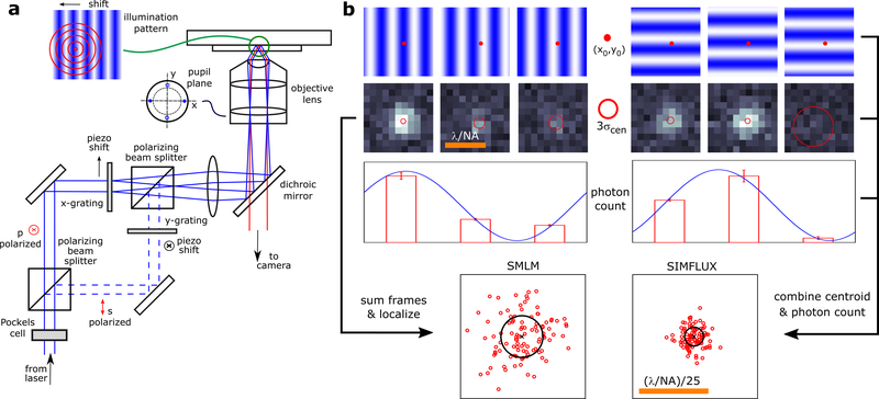
Figure 1 |
Principle of SIMFLUX. a, A sinusoidal illumination pattern is created in a Total Internal Reflection (TIRF)-SIM setup by two counter propagating evanescent waves. Fast switching between two orthogonal...
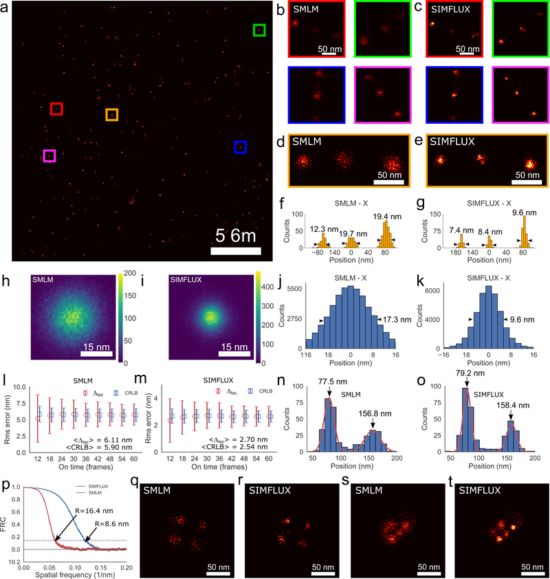
Figure 2 |
Demonstration of SIMFLUX on DNA-origami nano-stuctures. a, Full 26 u03bcm wide FOV SIMFLUX image of sparsely distributed nano-rulers with 80 nm spacing. Four independent imaging experiments were done ...
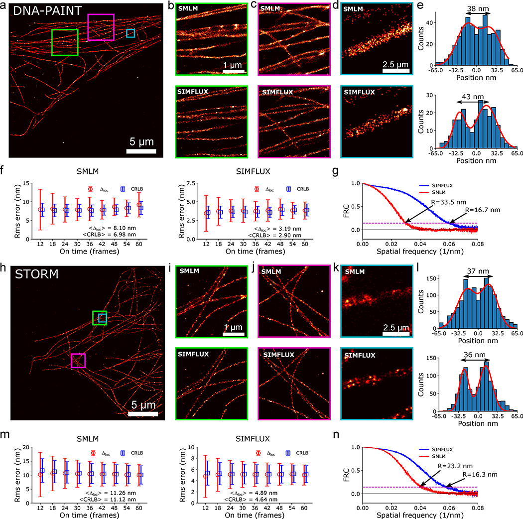
Figure 3 |
Demonstration of SIMFLUX on cellular tubulin with DNA-PAINT and (d)STORM. a, Full 26 u03bcm wide FOV SIMFLUX image of tubulin sample imaged with DNA-PAINT. Three independent imaging experiments were d...
Figure images are served from the NIH/NLM PubMed Central Open Access Subset or Europe PMC; copyright remains with the publishers and authors.
💬 Discussion
0 commentsNo comments yet. Be the first to start a discussion!
Leave a Comment