Abstract
Abstract Elucidating protein functions and molecular organisation requires to localise precisely single or aggregated molecules and analyse their spatial distributions. We develop a statistical method SODA (Statistical Object Distance Analysis) that uses either micro- or nanoscopy to significantly improve on standard co-localisation techniques. Our method considers cellular geometry and densities of molecules to provide statistical maps of isolated and associated (coupled) molecules. We use SODA with three-colour structured-illumination microscopy (SIM) images of hippocampal neurons, and statistically characterise spatial organisation of thousands of synapses. We show that presynaptic synapsin is arranged in asymmetric triangle with the 2 postsynaptic markers homer and PSD95, indicating a deeper localisation of homer. We then determine stoichiometry and distance between localisations of two synaptic vesicle proteins with 3D-STORM. These findings give insights into the protein organisation at the synapse, and prove the efficiency of SODA to quantitatively assess the geometry of molecular assemblies.
🔬 Techniques
🔭 Microscopes
✨ Fluorophores
🧪 Sample Preparation
🔬 Cell Lines
🏭 Microscope Brands
🧪 Reagent Suppliers
📷 Detectors
💻 Software Details
💾 Data Repositories
🏛️ Research Organizations (ROR)
Affiliated research institutions:
📋 Methods
Computation of G 0 The Ripley-based vector G is the sum of a normal vector documentclass[12pt]{minimal} usepackage{amsmath} usepackage{wasysym} usepackage{amsfonts} usepackage{amssymb} usepackage{amsbsy} usepackage{mathrsfs} usepackage{upgreek} setlength{oddsidemargin}{-69pt} begin{document}$${cal N}({boldsymbol{mu }},{boldsymbol{sigma }})$$end{document} N ( μ , σ ) that counts the number of random (red) objects in each ring, and of a coupled vector C that counts the additional number of coupled objects. The component C i of C counts the total number of (red) objects that are coupled to (green) objects inside Ring( r i , r i +1 ). We highlight that C i is an overestimate of the number of (red) A 2 objects with a coupling distance comprised between r i and r i +1 . Indeed, when (green) A 1 objects are densely packed, other (red) objects with different coupling distances that are coupled to (green) neighbors can also lay within Ring( r i , r i +1 ). We can thus decompose documentclass[12pt]{minimal} usepackage{amsmath} usepackage{wasysym} usepackage{amsfonts} usepackage{amssymb} usepackage{amsbsy} usepackage{mathrsfs} usepackage{upgreek} setlength{oddsidemargin}{-69pt} begin{document}$$C_i = widetilde C_i + mathop {sum}nolimits_{j ne i} {kern 1pt} alpha _{i,j}widetilde C_j$$end{document} C i = C ~ i + ∑ j ≠ i α i , j C ~ j , with documentclass[12pt]{minimal} usepackage{amsmath} usepackage{wasysym} usepackage{amsfonts} usepackage{amssymb} usepackage{amsbsy} usepackage{mathrsfs} usepackage{upgreek} setlength{oddsidemargin}{-69pt} begin{document}$$widetilde C_i$$end{document} C ~ i the exact number of couples with a coupling distance comprised between r i and r i +1 . The weighted sum documentclass[12pt]{minimal} usepackage{amsmath} usepackage{wasysym} usepackage{amsfonts} usepackage{amssymb} usepackage{amsbsy} usepackage{mathrsfs} usepackage{upgreek} setlength{oddsidemargin}{-69pt} begin{document}$$mathop {sum}nolimits_{j ne i} {kern 1pt} alpha _{i,j}tilde C_j$$end{document} ∑ j ≠ i α i , j C ~ j counts the total number of (red) coupled objects with coupling distance comprised between r j and r j +1 with j ≠ i but that lay within Ring( r i , r i +1 ) around some (green) objects. We highlight that this weighted contribution tends to 0 when (green) objects are well separated and do not share (red) couples. The weight α i , j is equal to the proportion of Rings( r i , r i +1 ) that overlap with Rings( r j , r j +1 ) around (green) A 1 objects. In a matrix form, the coupling decomposition reads documentclass[12pt]{minimal} usepackage{amsmath} usepackage{wasysym} usepackage{amsfonts} usepackage{amssymb} usepackage{amsbsy} usepackage{mathrsfs} usepackage{upgreek} setlength{oddsidemargin}{-69pt} begin{document}$${mathbf{C}} = {mathbf{A}}.{widetilde{mathbf C}}$$end{document} C = A . C ~ with A [ i , i ] = 1 and A [ i , j ≠ i ] = α i , j . To statistically estimate each component of the coupling vector documentclass[12pt]{minimal} usepackage{amsmath} usepackage{wasysym} usepackage{amsfonts} usepackage{amssymb} usepackage{amsbsy} usepackage{mathrsfs} usepackage{upgreek} setlength{oddsidemargin}{-69pt} begin{document}$${widetilde{mathbf C}}$$end{document} C ~ , we use the reduced Ripley’s vector documentclass[12pt]{minimal} usepackage{amsmath} usepackage{wasysym} usepackage{amsfonts} usepackage{amssymb} usepackage{amsbsy} usepackage{mathrsfs} usepackage{upgreek} setlength{oddsidemargin}{-69pt} begin{document}$${{mathbf G}^{mathbf{0}}} = frac{1}{boldsymbol{sigma} }{mathbf{A}}^{-1}.left[ {{mathbf G} - {boldsymbol{mu }}} right]$$end{document} G 0 = 1 σ A - 1 . G - μ . Indeed, under the null hypothesis of (red) objects’ randomness, G 0 is a Gaussian vector with zero mean and unit variance. Moreover σ G 0 is proportional to the number of couples documentclass[12pt]{minimal} usepackage{amsmath} usepackage{wasysym} usepackage{amsfonts} usepackage{amssymb} usepackage{amsbsy} usepackage{mathrsfs} usepackage{upgreek} setlength{oddsidemargin}{-69pt} begin{document}$${widetilde{mathbf C}}$$end{document} C ~ at different distances, and thereof, it can be used to compute the coupling probability for each individual pair of objects.
Show full methods section
Computation of G 0 The Ripley-based vector G is the sum of a normal vector documentclass[12pt]{minimal} usepackage{amsmath} usepackage{wasysym} usepackage{amsfonts} usepackage{amssymb} usepackage{amsbsy} usepackage{mathrsfs} usepackage{upgreek} setlength{oddsidemargin}{-69pt} begin{document}$${cal N}({boldsymbol{mu }},{boldsymbol{sigma }})$$end{document} N ( μ , σ ) that counts the number of random (red) objects in each ring, and of a coupled vector C that counts the additional number of coupled objects. The component C i of C counts the total number of (red) objects that are coupled to (green) objects inside Ring( r i , r i +1 ). We highlight that C i is an overestimate of the number of (red) A 2 objects with a coupling distance comprised between r i and r i +1 . Indeed, when (green) A 1 objects are densely packed, other (red) objects with different coupling distances that are coupled to (green) neighbors can also lay within Ring( r i , r i +1 ). We can thus decompose documentclass[12pt]{minimal} usepackage{amsmath} usepackage{wasysym} usepackage{amsfonts} usepackage{amssymb} usepackage{amsbsy} usepackage{mathrsfs} usepackage{upgreek} setlength{oddsidemargin}{-69pt} begin{document}$$C_i = widetilde C_i + mathop {sum}nolimits_{j ne i} {kern 1pt} alpha _{i,j}widetilde C_j$$end{document} C i = C ~ i + ∑ j ≠ i α i , j C ~ j , with documentclass[12pt]{minimal} usepackage{amsmath} usepackage{wasysym} usepackage{amsfonts} usepackage{amssymb} usepackage{amsbsy} usepackage{mathrsfs} usepackage{upgreek} setlength{oddsidemargin}{-69pt} begin{document}$$widetilde C_i$$end{document} C ~ i the exact number of couples with a coupling distance comprised between r i and r i +1 . The weighted sum documentclass[12pt]{minimal} usepackage{amsmath} usepackage{wasysym} usepackage{amsfonts} usepackage{amssymb} usepackage{amsbsy} usepackage{mathrsfs} usepackage{upgreek} setlength{oddsidemargin}{-69pt} begin{document}$$mathop {sum}nolimits_{j ne i} {kern 1pt} alpha _{i,j}tilde C_j$$end{document} ∑ j ≠ i α i , j C ~ j counts the total number of (red) coupled objects with coupling distance comprised between r j and r j +1 with j ≠ i but that lay within Ring( r i , r i +1 ) around some (green) objects. We highlight that this weighted contribution tends to 0 when (green) objects are well separated and do not share (red) couples. The weight α i , j is equal to the proportion of Rings( r i , r i +1 ) that overlap with Rings( r j , r j +1 ) around (green) A 1 objects. In a matrix form, the coupling decomposition reads documentclass[12pt]{minimal} usepackage{amsmath} usepackage{wasysym} usepackage{amsfonts} usepackage{amssymb} usepackage{amsbsy} usepackage{mathrsfs} usepackage{upgreek} setlength{oddsidemargin}{-69pt} begin{document}$${mathbf{C}} = {mathbf{A}}.{widetilde{mathbf C}}$$end{document} C = A . C ~ with A [ i , i ] = 1 and A [ i , j ≠ i ] = α i , j . To statistically estimate each component of the coupling vector documentclass[12pt]{minimal} usepackage{amsmath} usepackage{wasysym} usepackage{amsfonts} usepackage{amssymb} usepackage{amsbsy} usepackage{mathrsfs} usepackage{upgreek} setlength{oddsidemargin}{-69pt} begin{document}$${widetilde{mathbf C}}$$end{document} C ~ , we use the reduced Ripley’s vector documentclass[12pt]{minimal} usepackage{amsmath} usepackage{wasysym} usepackage{amsfonts} usepackage{amssymb} usepackage{amsbsy} usepackage{mathrsfs} usepackage{upgreek} setlength{oddsidemargin}{-69pt} begin{document}$${{mathbf G}^{mathbf{0}}} = frac{1}{boldsymbol{sigma} }{mathbf{A}}^{-1}.left[ {{mathbf G} - {boldsymbol{mu }}} right]$$end{document} G 0 = 1 σ A - 1 . G - μ . Indeed, under the null hypothesis of (red) objects’ randomness, G 0 is a Gaussian vector with zero mean and unit variance. Moreover σ G 0 is proportional to the number of couples documentclass[12pt]{minimal} usepackage{amsmath} usepackage{wasysym} usepackage{amsfonts} usepackage{amssymb} usepackage{amsbsy} usepackage{mathrsfs} usepackage{upgreek} setlength{oddsidemargin}{-69pt} begin{document}$${widetilde{mathbf C}}$$end{document} C ~ at different distances, and thereof, it can be used to compute the coupling probability for each individual pair of objects.
Estimation of the coupling probability
P (x, y) Each component G i of the Ripley-based vector G is proportional to the number of (red) objects A 2 that lay within Ring( r i , r i +1 ) around (green) objects A 1 (Table 2 ), and the total number of (red) objects within Ring( r i , r i +1 ) is given by 4 documentclass[12pt]{minimal} usepackage{amsmath} usepackage{wasysym} usepackage{amsfonts} usepackage{amssymb} usepackage{amsbsy} usepackage{mathrsfs} usepackage{upgreek} setlength{oddsidemargin}{-69pt} begin{document}$$begin{array}{l}{mathrm{Total}},{mathrm{Number}},{mathrm{of}},({mathrm{red}}),{mathrm{objects}},{mathrm{in}},mathrm{Ring}(r_i,r_{i + 1}) = frac{{n_1n_2}}{{{mathrm{Volume}},{mathrm{of}},{mathrm{the}},{mathrm{ROI}}}}G_i.end{array}$$end{document} Total Number of ( red ) objects in Ring ( r i , r i + 1 ) = n 1 n 2 Volume of the ROI G i . On the other hand, the number documentclass[12pt]{minimal} usepackage{amsmath} usepackage{wasysym} usepackage{amsfonts} usepackage{amssymb} usepackage{amsbsy} usepackage{mathrsfs} usepackage{upgreek} setlength{oddsidemargin}{-69pt} begin{document}$$widetilde C_i$$end{document} C ~ i of (red) coupled objects inside Ring( r i , r i +1 ), after correction of rings’ overlap, is given by 5 documentclass[12pt]{minimal} usepackage{amsmath} usepackage{wasysym} usepackage{amsfonts} usepackage{amssymb} usepackage{amsbsy} usepackage{mathrsfs} usepackage{upgreek} setlength{oddsidemargin}{-69pt} begin{document}$$widetilde C_i = frac{{n_1n_2sigma _i{G}_i^0}}{{{mathrm{Volume}},{mathrm{of}},{mathrm{the}},{mathrm{ROI}}}}{mathbf{1}}left{ {{G}_i^0 > T(N)} right}.$$end{document} C ~ i = n 1 n 2 σ i G i 0 Volume of the ROI 1 G i 0 > T ( N ) . Thus, the coupling probability P ( x , y ) between a (green) object located at position x and a (red) object located at position y is equal to 6 documentclass[12pt]{minimal} usepackage{amsmath} usepackage{wasysym} usepackage{amsfonts} usepackage{amssymb} usepackage{amsbsy} usepackage{mathrsfs} usepackage{upgreek} setlength{oddsidemargin}{-69pt} begin{document}$$begin{array}{*{20}{l}} {P({mathbf{x}},{mathbf{y}})} hfill & = hfill & {mathop {sum}limits_{i = 0}^{N - 1} {kern 1pt} {mathbf{1}}left{ {r_i < d({mathbf{x}},{mathbf{y}}) le r_{i + 1}} right}} {} {} { times {displaystylefrac{{widetilde C_i}}{{mathrm{Total}},{mathrm{Number}},{mathrm{of}},({mathrm{red}}),{mathrm{objects}},{mathrm{in}},mathrm{Ring}(r_i,r_{i + 1})}}} hfill \ {} hfill & = hfill & {mathop {sum}limits_{i = 0}^{N - 1} {mathbf{1}}left{ {r_i < d({mathbf{x}},{mathbf{y}}) le r_{i + 1}} right}frac{{sigma _iG_i^0{mathbf{1}}left{ {G_i^0 > T(N)} right}}}{{G_i}}.} hfill end{array}$$end{document} P ( x , y ) = ∑ i = 0 N - 1 1 r i < d ( x , y ) ≤ r i + 1 × C ~ i Total Number of ( red ) objects in Ring ( r i , r i + 1 ) = ∑ i = 0 N - 1 1 r i < d ( x , y ) ≤ r i + 1 σ i G i 0 1 G i 0 > T ( N ) G i .
Statistical test of spot coupling
To build a statistical test of objects’ coupling, we use the reduced vector G 0 and use the maximal component documentclass[12pt]{minimal} usepackage{amsmath} usepackage{wasysym} usepackage{amsfonts} usepackage{amssymb} usepackage{amsbsy} usepackage{mathrsfs} usepackage{upgreek} setlength{oddsidemargin}{-69pt} begin{document}$${G}_{{mathrm{max}}}^0 = {mathrm{sup}}_{1 le i le N - 1}{kern 1pt} {G}_0^i$$end{document} G max 0 = sup 1 ≤ i ≤ N - 1 G 0 i to test statistically whether (red) objects are randomly distributed (null hypothesis), or if there is at least one ring where coupled objects accumulate significantly. For any x > 0, we have that 7 documentclass[12pt]{minimal} usepackage{amsmath} usepackage{wasysym} usepackage{amsfonts} usepackage{amssymb} usepackage{amsbsy} usepackage{mathrsfs} usepackage{upgreek} setlength{oddsidemargin}{-69pt} begin{document}$$begin{array}{*{20}{l}} {{mathrm{Pr}}left{ {{G}_{{mathrm{max}}}^0 ge x} right}} hfill & = hfill & {1 - {mathrm{Pr}}left{ {{G}_{{mathrm{max}}}^0 < x} right}} hfill \ {} hfill & = hfill & {1 - {mathrm{Pr}}left{ {forall i,0 le i le N - 1,{G}_i^0 < x} right}.} hfill end{array}$$end{document} Pr G max 0 ≥ x = 1 - Pr G max 0 < x = 1 - Pr ∀ i , 0 ≤ i ≤ N - 1 , G i 0 < x . Because documentclass[12pt]{minimal} usepackage{amsmath} usepackage{wasysym} usepackage{amsfonts} usepackage{amssymb} usepackage{amsbsy} usepackage{mathrsfs} usepackage{upgreek} setlength{oddsidemargin}{-69pt} begin{document}$$G_i^0$$end{document} G i 0 , for 0 ≤ i ≤ N − 1, are independent normal variables, we have 8 documentclass[12pt]{minimal} usepackage{amsmath} usepackage{wasysym} usepackage{amsfonts} usepackage{amssymb} usepackage{amsbsy} usepackage{mathrsfs} usepackage{upgreek} setlength{oddsidemargin}{-69pt} begin{document}$${mathrm{Pr}}left{ {forall i,0 le i le N - 1,{G}_i^0 < x} right} = left( {{mathrm{Pr}}left{ {{cal N}(0.1) < x} right}} right)^N,$$end{document} Pr ∀ i , 0 ≤ i ≤ N - 1 , G i 0 < x = Pr N ( 0.1 ) < x N , that is 9 documentclass[12pt]{minimal} usepackage{amsmath} usepackage{wasysym} usepackage{amsfonts} usepackage{amssymb} usepackage{amsbsy} usepackage{mathrsfs} usepackage{upgreek} setlength{oddsidemargin}{-69pt} begin{document}$${mathrm{Pr}}left{ {forall i,0 le j le N - 1,{G}_i^0 < x} right} = {mathrm{cdf}}^N(x),$$end{document} Pr ∀ i , 0 ≤ j ≤ N - 1 , G i 0 < x = cdf N ( x ) , where cdf( x ) is the cumulative density function of the standard normal law: documentclass[12pt]{minimal} usepackage{amsmath} usepackage{wasysym} usepackage{amsfonts} usepackage{amssymb} usepackage{amsbsy} usepackage{mathrsfs} usepackage{upgreek} setlength{oddsidemargin}{-69pt} begin{document}$${mathrm{cdf}}(x) = {int}_{ - infty }^x {kern 1pt} frac{1}{{sqrt {2pi } }}{kern 1pt} {mathrm{exp}}^{ - frac{{x^2}}{2}}dx$$end{document} cdf ( x ) = ∫ - ∞ x 1 2 π exp - x 2 2 d x . Finally, reinjecting Eq. ( 9 ) in Eq. ( 7 ), we obtain that 10 documentclass[12pt]{minimal} usepackage{amsmath} usepackage{wasysym} usepackage{amsfonts} usepackage{amssymb} usepackage{amsbsy} usepackage{mathrsfs} usepackage{upgreek} setlength{oddsidemargin}{-69pt} begin{document}$${mathrm{Pr}}left{ {{G}_{{mathrm{max}}}^0 ge x} right} = 1 - {mathrm{cdf}}^N(x),$$end{document} Pr G max 0 ≥ x = 1 - cdf N ( x ) , and the p- value is thus given by 11 documentclass[12pt]{minimal} usepackage{amsmath} usepackage{wasysym} usepackage{amsfonts} usepackage{amssymb} usepackage{amsbsy} usepackage{mathrsfs} usepackage{upgreek} setlength{oddsidemargin}{-69pt} begin{document}$${{ptext{-}}}{mathrm{value}} = 1 - {mathrm{cdf}}^N(G_{{mathrm{max}}}^0).$$end{document} p - value = 1 - cdf N ( G max 0 ) .
Gaussian point process simulations
In simulations, we use a Gaussian point processes where positions of coupled (red) points (=localisations) are distributed around (green) points. The radial coupling distance r , in turn, follows the absolute value of a normal law: r = | u | with documentclass[12pt]{minimal} usepackage{amsmath} usepackage{wasysym} usepackage{amsfonts} usepackage{amssymb} usepackage{amsbsy} usepackage{mathrsfs} usepackage{upgreek} setlength{oddsidemargin}{-69pt} begin{document}$$u sim {cal N}(mu _c,sigma _c)$$end{document} u ~ N ( μ c , σ c ) . For STORM imaging, we also add an upper-bound (threshold) for the radial distance r < 80 nm. The mean μ c models the mean coupling distance between points and accounts for the type of coupling (direct interaction, synaptic apposition…) between molecules (Fig. 1 ). The s.d. σ c , in turn, accounts for both the possible variations in the interaction distance due to thermal noise or organelle size for example, and the localisation’ uncertainty.
Generation of synthetic images
We use a Mixed Poisson-Gaussian model to generate synthetic fluorescent images with size 256 × 256 pixels and a number n 1 = n 2 = 100 of fluorescent spots (chapter 1 of ref. 59 ). In this model, the intensity I [ x , y ] at pixel location [ x , y ] is equal to documentclass[12pt]{minimal} usepackage{amsmath} usepackage{wasysym} usepackage{amsfonts} usepackage{amssymb} usepackage{amsbsy} usepackage{mathrsfs} usepackage{upgreek} setlength{oddsidemargin}{-69pt} begin{document}$$I[x,y] = {mathrm{gain}} ast U[x,y] + N(x,y)$$end{document} I [ x , y ] = gain * U [ x , y ] + N ( x , y ) where U is a random Poisson variable and N an additive white Gaussian noise with mean 0 and s.d. equal to σ N . The mean λ [ x , y ] of the Poisson variable U varies spatially: λ [ x , y ] = P [ x , y ] + B , P [ x , y ] being the sum of the intensity of the particles generated in [ x , y ] and B = 50 a constant background value. gain = 1 is the gain of the acquisition system. Finally, we assume an additive model for the intensity of the particles: documentclass[12pt]{minimal} usepackage{amsmath} usepackage{wasysym} usepackage{amsfonts} usepackage{amssymb} usepackage{amsbsy} usepackage{mathrsfs} usepackage{upgreek} setlength{oddsidemargin}{-69pt} begin{document}$$P[x,y] = mathop {sum}nolimits_{i = 1}^N {kern 1pt} P_i[x,y]$$end{document} P [ x , y ] = ∑ i = 1 N P i [ x , y ] , where P i [ x , y ] is the signal originating from the i th particle in pixel [ x , y ]. When a particle is significantly smaller than the resolution of the microscope, its intensity profile P i is well represented by the Gaussian PSF of the microscope 60 with a specific amplitude A i : documentclass[12pt]{minimal} usepackage{amsmath} usepackage{wasysym} usepackage{amsfonts} usepackage{amssymb} usepackage{amsbsy} usepackage{mathrsfs} usepackage{upgreek} setlength{oddsidemargin}{-69pt} begin{document}$$P_i[x,y] = A_ie^{ - frac{{left( {x - x_i^0} right)^2 + left( {y - y_i^0} right)^2}}{{2sigma _{xy}^2}}}$$end{document} P i [ x , y ] = A i e - x - x i 0 2 + y - y i 0 2 2 σ x y 2 where documentclass[12pt]{minimal} usepackage{amsmath} usepackage{wasysym} usepackage{amsfonts} usepackage{amssymb} usepackage{amsbsy} usepackage{mathrsfs} usepackage{upgreek} setlength{oddsidemargin}{-69pt} begin{document}$$left[ {x_i^0,y_i^0} right]$$end{document} x i 0 , y i 0 is the coordinate of the i th particle and σ xy the s.d. of the 2D Gaussian profile of the PSF. Particle amplitude A i was fixed to A i = 100 for each particle 1 ≤ i ≤ N . Finally, the s.d. σ N of the white Gaussian noise is computed based on the targeted SNR value 59 : documentclass[12pt]{minimal} usepackage{amsmath} usepackage{wasysym} usepackage{amsfonts} usepackage{amssymb} usepackage{amsbsy} usepackage{mathrsfs} usepackage{upgreek} setlength{oddsidemargin}{-69pt} begin{document}$$SNR = frac{{A_i}}{{A_i + B + sigma _N^2}}$$end{document} S N R = A i A i + B + σ N 2 , leading to documentclass[12pt]{minimal} usepackage{amsmath} usepackage{wasysym} usepackage{amsfonts} usepackage{amssymb} usepackage{amsbsy} usepackage{mathrsfs} usepackage{upgreek} setlength{oddsidemargin}{-69pt} begin{document}$$sigma _N = sqrt {frac{{A_i^2}}{{SNR^2}} - (A_i + B)}$$end{document} σ N = A i 2 S N R 2 - ( A i + B ) . Automatic segmentation of putative synaptic boutons To delineate automatically volumes where VGLUT and Synapsin are densely packed (and thus ignore isolated, background localisations), we adapt the Density-Based Spatial Clustering of Applications with Noise (DBSCAN) method 52 , and implemented it in Icy. We thus define an ensemble of core points that have more than m = 10 neighbors at a distance below d = 200 nm. m and d are user-defined parameters, and we checked that the ensemble of core points was not affected too much by variations of these parameters. Then, we build the ROIs around densely packed localisations by taking the union of balls centred at computed core points with radius d + δ , where δ is a dilatation parameter that smoothen the ROI’s boundaries ( d = δ here). Finally, the ROI corresponding to putative synaptic boutons and used to perform the coupling analysis with SODA is equal to the boolean intersection of VGLUT and Synapsin ROIs.
Icy protocols
We perform multi-steps batch analysis of SIM and STORM images using graphical programming plugin Protocols in Icy. Tutorial for Icy installation is provided (Supplementary Movie 2 ). Protocols’ screenshots are shown in Supplementary Figs 3 and 4, and are publicly available on Icy website ( http://icy.bioimageanalysis.org/protocol/list ). Protocols’ tutorials are provided as Supplementary Movies 3 and 4 . Each protocol consists of multiple elementary blocks that perform sequential steps of the image analysis. SIM protocol (Supplementary Fig. 3 and Supplementary Movie 3 (tutorial)): First, user specifies the folder that contains multichannel SIM images, and defines inputs of the protocol such as the channels of pre- and postsynaptic molecules, the channel used to define the dendritic mask, the scales and thresholds used in the wavelet detection of molecule spots 9 or the maximal search distance of SODA. Then a first series of blocks in the protocol delineate the dendritic mask (block 6, can be expanded by double-clicking on the block title Cell Mask). It consists of HK-means thresholding of the fluorescence intensity of the pre-defined image channels to segment the whole neuron and the brighter cell soma. Dendritic mask is then obtained by removing the soma mask to the neuronal mask. The mask is then dilated to cover also presynaptic Synapsin spots in adjacent axons. The second main step of SODA protocol consists of wavelet detection blocks (blocks 10-14-19) 9 to extract pre- and postsynaptic spots inside the dendritic mask. The next three blocks (16-20-24) of the protocol are the specific SODA block that statistically analyse the coupling between PSD95 and Homer, PSD95 and Synapsin, and Homer and Synapsin respectively. Based on SODA analysis, we designed a specific block (32) named Trio to extract single isolated spots, couples and triplets, with their individual morphologies and the associated coupling probabilities and distances. Triplets are defined as ensembles of three different spots (Homer, PSD95 and Synapsin) with at least two strictly positive coupling probabilities among the three. An option in the block Trio "Select strict triplets" allows to select only triplets with three positive coupling probabilities (in our experiment, there are 3129 strict triplets, and 7930 triplets with at least two positive coupling probabilities). STORM protocol (Supplementary Fig. 4 Supplementary Movie 4 (tutorial)): A first series of blocks (blocks 5–7) extract localisations’ coordinates from microscope files. Then, a second series of blocks delineate three-dimensional ROIs around dense clusters of VGLUT and Synapsin localisations using the DBSCAN method (blocks 6–8). The intersection between VGLUT and Synapsin ROIs (block 9) is, with single-molecule localisations, an input of the SODA STORM 3D block (10) that statistically computes all the coupling probabilities between individual VGLUT and Synapsin localisations. Finally, a last series of blocks export SODA results (coupling parameters) in files (block 11) and map single and coupled localisations in 3D with VTK ( http://www.vtk.org ) in Icy (blocks 12-13-14 and 15).
Generation of genome-edited cells and fluorescence staining
Hep2, a Human cervical adenocarcinoma cell line (Clone 2B, misidentified BioSample: SAMN03151705) was a gift of A Dautry and was the parental cell line used to obtain the clone Hep2 β , stably expressing IL-2Rβ gene as described in (Grassart et al. EMBO R, 2008). This cell line did not have any mycoplasma contamination as verified by the kit MycoAlert from Lonza. Hep2β cells were edited for CLTA similarly to clathrin-GFP edited cells 61 : Briefly, Zinc-Finger-Nucleases (ZFNs) and donor plasmids were transfected into cells using a single cuvette Amaxa Nucleofector device (Lonza), as per the manufacturer’s protocol, Nucleofector solution R and programme I-013. After transfection, cells were transferred to 37 °C, 5% CO 2 . Recovered cells were sorted for GFP-positive signals using a DAKO-Cytomation MoFlo High Speed Sorter directly as single cells into 96-well plates. Cells were maintained under 5% CO2 at 37 °C in DMEM (Invitrogen) supplemented with 10% FBS (Biowest). Cells were grown on glass bottom dishes No 1.5 (MatTekTM) overnight and incubated the next day for 2 min at 37 °C with transferrin (Sigma-aldrich ref: T0665) coupled to Cy3 (house-made coupling with Fluorochrome CY3 monofunctional (GE Healthcare, Ref: Q13108 )), or with house-made anti-IL2R 561 62 coupled to Cy3 (house-made coupling with Fluorochrome CY3 monofunctional (GE Healthcare, Ref: Q13108 )) for 5 min. Then, cells were extensively washed and immediately fixed in 4% paraformaldehyde and 4% sucrose at room temperature for 20 min.
Primary hippocampal neurons in culture
Hippocampal cultures were obtained from 18-day-old mice (C57BL6N) or rat (Sprague Dawley) embryos. All male and female embryos were used and mixed per litter (usually from 6–8 for mice to 10–12 for rats). Similarly to ref. 63 , hippocampi from E18 rodent embryos were dissociated by treatment with trypsin (0.25% for 15 min at 37 °C) followed by trituration with a constricted Pasteur pipette. The cells were plated onto poly-Ornithine-coated coverslips (1 mg/mL) (Sigma-Aldrich, St. Louis, MO) in 4-well tissue culture plates at density of 6 × 10 4 cells/well in MEM-HS medium (modified Eagles medium, 10% horse serum, 0.06% glucose, 100 units/mL penicillin, 100 μg/mL streptomycin, 500 μM Glutamax). After 1 h, when the cells were attached to the substrate, the medium was replaced with Neurobasal-B27 medium conditioned previously on confluent glial feeder layer (neurobasal medium (Gibco) containing 2% B27 supplement (Gibco), and 500 μ M L-Glutamine (Sigma-Aldrich). Cultures were maintained 3 weeks at 37 °C in a humidified atmosphere of 95% air and 5% CO 2 to obtain mature hippocampal network and synapses. Neurobasal medium was conditioned overnight on a confluent astrocyte feeder layer. One third of the neuronal medium was then replaced with this fresh conditioned medium once a week.
Immunohistochemistry
Similarly to ref. 41 , neurons were fixed with cold methanol for 5 min at −20 °C. Quenching with NH4Cl for 15 min was followed by a permeabilisation step for 4 min with a mixture of 0.1% Triton-X100/PBS/0.125% cold water fish skin gelatin (fish gelatin) (Sigma-Aldrich). After three PBS 1× washings, neurons were incubated in blocking solution containing PBS/0.25% fish gelatin for 30 min. Immunocytological staining was performed by incubation with the primary antibody in PBS/0.125% fish gelatin overnight at 4 °C, followed by an incubation in the secondary antibody in PBS/0.125% fish gelatin for 45 min at room temperature. The antibodies used were: guinea pig polyclonal antibody to Synapsin (synapsin 1/2 (#106004), dilution 2000e) and rabbit polyclonal anti-Homer (Homer 1(#160003), 200e) were from Synaptic Systems, mouse monoclonal anti-PSD95 (# P78352 , 500e) was from NeuromAb, chicken polyclonal anti-MAP2 (#ab5392, 20000e) was from Abcam, and VGLUT1&2 antibody (#pab0047, 200e) was from Covalab 64 .
Total internal reflection fluorescence microscopy
Total internal reflection fluorescence (TIRF) microscopy images were captured using Cell MTM software on an Olympus IX-81 microscope using a 100x/NA1.45 objective and an EMCCD camera IxonEM+ (Andor). A 488 nm solid-state laser (Olympus) and a 561 nm solid-state laser (Olympus) were used to excite GFP and Cy3 fluorophores, respectively. Images were obtained without gain and an exposure time of 800 to 1000 ms. Simultaneous two colour TIRF images were obtained using a DV2 image splitter (Optical Insights) to separate GFP and Cy3 emission signals.
Confocal microscopy
Confocal images for synaptic triple labelling were obtained using a confocal microscope Leica TCS SP5 (Leica Microsystems CMS GmbH, Mannheim, Germany) and a ×63 objective (NA 1.4; followed by a digital zoom to achieve the ideal sampling). Images were acquired by sequential scanning of the emission lines. Alexa 488 was detected using the 488 nm-line of an argon laser for excitation; Cy3 and Cy5 were respectively excited by the 543 nm-line of a green neon laser and the 633 nm-line of a helium neon laser. Typically, sections (from 1024 up to 4096 pixels), were scanned three times, to optimise the signal/noise ratio.
Structured-illumination microscopy
Super-resolution structured-illumination microscopy
(SIM) was performed on a Zeiss Elyra PS.1 system equipped with a 63x objective (N.A. 1.4) and an EMCCD Andor, iXon 885 camera. Three channels containing pictures (typically 1900 × 1900 pixels with a pixel size of 39 nm) were acquired with 4 lasers (405, 488, 561 and 642 nm) and five different grids. Quantification was performed on 9 neurons for each condition which correspond roughly to 20,000 to 30,000 immunoreactive spots for each channels. Statistical significance was evaluated using Graphpad prism software. The level of significance (Mann-Whitney) is indicated by one ( p < 0.05), two ( p < 0.01), or three ( p < 0.001) symbols.
Stochastic optical reconstruction microscopy
Stochastic optical reconstruction microscopy
(STORM) imaging was performed on a Vutara microscope (Bruker) with a high-numerical aperture (NA) objective (60x, water, NA 1.2, Olympus). 170 nm coverslips (Menzel glaser 18 mm diameter #1.5) were mounted on a glass slide with a 15mm hole. The hole was filled with imaging buffer (Tris 50 mM, NaCl 10 mM, 10% glucose, 100 mM MEA, 70 U/mL glucose oxidase (Sigma G0543), 20 g/mL catalase) and sealed with Picodent twinsil. Samples were illuminated successively with a 647 and 488 nm laser and a 405 nm laser for the reactivation of the 488 fluorophores. Neurons were isolated with wide field mosaïc microscopy (Cool snap camera) and then imaged for STORM for a series of 30 000 images with a FLASH4 CMOS camera (20 ms, 20 × 20 microns). 3D-STORM imaging was done using the bi-plane module allowing the localisation in the xyz direction. The Srx software (Bruker) was used to localise particles in 3D. Localisation tables were exported and used in ICY software for statistical localisation analysis. Correction for chromatic aberration TIRF images have been corrected using beads’ alignment with rigid registration (plugin Rigid registration in Icy) and then, (inverse) rigid transformation of images.
Correction for chromatic aberration in super-resolution microscopy
(SIM and STORM) has been done using multispectral (blue/green/orange/dark red) Tetraspeck beads (Thermofisher T7279). Channel alignment has been done on SIM in Zeiss software or on STORM in Bruker’s software. Code availability Code (Icy protocols and plugins) can be freely dowloaded from Icy website ( http://icy.bioimageanalysis.org/list ) or directly within Icy software through the search bar.
Data availability
All data generated or analysed during this study are included in this published article (and its supplementary information files), or are available from the authors on reasonable request.
Icy protocols
We perform multi-steps batch analysis of SIM and STORM images using graphical programming plugin Protocols in Icy. Tutorial for Icy installation is provided (Supplementary Movie 2 ). Protocols’ screenshots are shown in Supplementary Figs 3 and 4, and are publicly available on Icy website ( http://icy.bioimageanalysis.org/protocol/list ). Protocols’ tutorials are provided as Supplementary Movies 3 and 4 . Each protocol consists of multiple elementary blocks that perform sequential steps of the image analysis. SIM protocol (Supplementary Fig. 3 and Supplementary Movie 3 (tutorial)): First, user specifies the folder that contains multichannel SIM images, and defines inputs of the protocol such as the channels of pre- and postsynaptic molecules, the channel used to define the dendritic mask, the scales and thresholds used in the wavelet detection of molecule spots 9 or the maximal search distance of SODA. Then a first series of blocks in the protocol delineate the dendritic mask (block 6, can be expanded by double-clicking on the block title Cell Mask). It consists of HK-means thresholding of the fluorescence intensity of the pre-defined image channels to segment the whole neuron and the brighter cell soma. Dendritic mask is then obtained by removing the soma mask to the neuronal mask. The mask is then dilated to cover also presynaptic Synapsin spots in adjacent axons. The second main step of SODA protocol consists of wavelet detection blocks (blocks 10-14-19) 9 to extract pre- and postsynaptic spots inside the dendritic mask. The next three blocks (16-20-24) of the protocol are the specific SODA block that statistically analyse the coupling between PSD95 and Homer, PSD95 and Synapsin, and Homer and Synapsin respectively. Based on SODA analysis, we designed a specific block (32) named Trio to extract single isolated spots, couples and triplets, with their individual morphologies and the associated coupling probabilities and distances. Triplets are defined as ensembles of three different spots (Homer, PSD95 and Synapsin) with at least two strictly positive coupling probabilities among the three. An option in the block Trio "Select strict triplets" allows to select only triplets with three positive coupling probabilities (in our experiment, there are 3129 strict triplets, and 7930 triplets with at least two positive coupling probabilities). STORM protocol (Supplementary Fig. 4 Supplementary Movie 4 (tutorial)): A first series of blocks (blocks 5–7) extract localisations’ coordinates from microscope files. Then, a second series of blocks delineate three-dimensional ROIs around dense clusters of VGLUT and Synapsin localisations using the DBSCAN method (blocks 6–8). The intersection between VGLUT and Synapsin ROIs (block 9) is, with single-molecule localisations, an input of the SODA STORM 3D block (10) that statistically computes all the coupling probabilities between individual VGLUT and Synapsin localisations. Finally, a last series of blocks export SODA results (coupling parameters) in files (block 11) and map single and coupled localisations in 3D with VTK ( http://www.vtk.org ) in Icy (blocks 12-13-14 and 15).
Electronic supplementary material Supplementary Information Peer Review File Description of Additional Supplementary Files Supplementary Movie 1 Supplementary Movie 2 Supplementary Movie 3 Supplementary Movie 4
📊 Figures
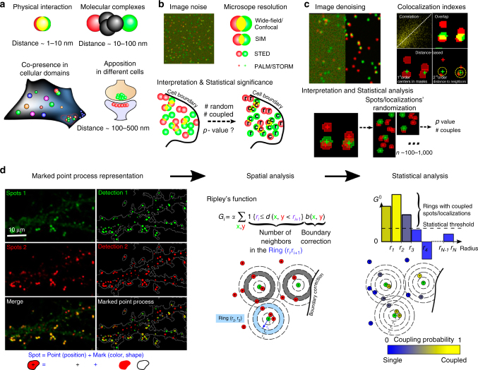
Fig. 1
Co-localisation analysis of moleculesu2019 coupling. a Moleculesu2019 coupling embraces direct interaction (distance <10u2009nm), indirect interaction inside a macromolecular complex (distance betw...
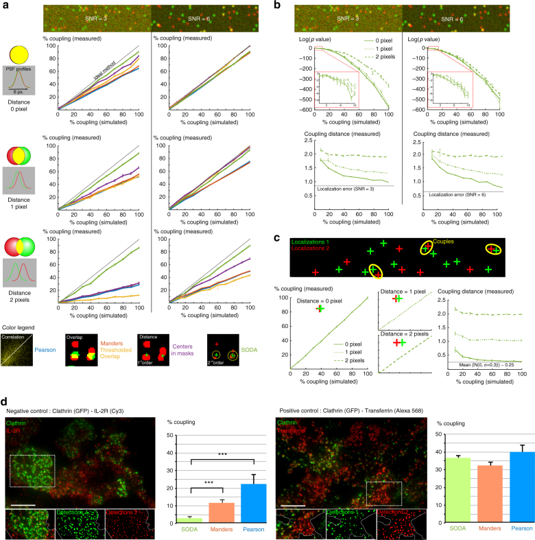
Fig. 2
Validation of SODA a Synthetic fluorescent images with different SNR and coupling parameters are generated (Material and Methods). SODA is compared with main coupling indexes (see Table 1 ): Pearson c...
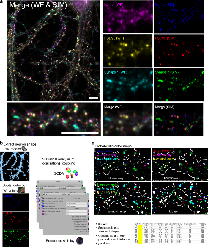
Fig. 3
Batch analysis using graphical programming in Icy. a The input of SODA protocol is a folder that contains multiple three-colour SIM images of primary hippocampal neurons. Postsynaptic anchoring molecu...
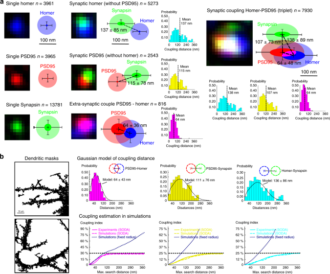
Fig. 4
A statistical view on glutamatergic synapse morphometry. a Using SODA protocol, the coupling of n =u200911200 PSD95, n =u200913359 Homer and n =u200926505 Synapsin spots among N =u20099 neurons is map...
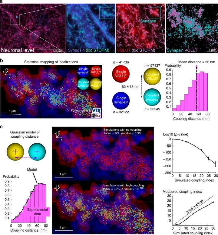
Fig. 5
Combining SODA and 3D-STORM imaging to map the coupling between VGLUT and Synapsin localisations inside presynaptic boutons. a VGLUT and Synapsin are imaged in cultured hippocampal neurons of mice wit...
Figure images are served from the NIH/NLM PubMed Central Open Access Subset or Europe PMC; copyright remains with the publishers and authors.
💬 Discussion
0 commentsNo comments yet. Be the first to start a discussion!
Leave a Comment