Abstract
AbstractImaging based on blood flow dynamics is widely used to study sensory processing. Here we investigated the extent to which local neuronal and capillary responses (two-photon microscopy) are correlated to mesoscopic responses detected with fast ultrasound (fUS) and BOLD-fMRI. Using a specialized chronic olfactory bulb preparation, we report that sequential imaging of the same mouse allows quantitative comparison of odour responses, imaged at both microscopic and mesoscopic scales. Under these conditions, functional hyperaemia occurred at the threshold of neuronal activation and fUS-CBV signals could be detected at the level of single voxels with activation maps varying according to blood velocity. Both neuronal and vascular responses increase non-linearly as a function of odour concentration, whereas both microscopic and mesoscopic vascular responses are linearly correlated to local neuronal calcium. These data establish strengths and limits of mesoscopic imaging techniques to report neural activity.
🔬 Techniques
✨ Fluorophores
🧪 Sample Preparation
🏭 Microscope Brands
🧪 Reagent Suppliers
📷 Detectors
💻 Software Details
🏛️ Research Organizations (ROR)
Affiliated research institutions:
📋 Methods
Animal preparation
All animal care and experimentation was performed in accordance with the INSERM Animal Care and Use Committee guidelines (protocol numbers CEEA34.SC.122.12 and CEEA34.SC.123.12). Adult mice ( n = 13, 2–12 months old, 20–35 g, both males and female, housed in 12-h light-dark cycle, fed ad libitum) were used in this study. Thy1 -GCaMP6f (GP5.11) mice were obtained from Jackson laboratory. For chronic craniotomies 28 mice were initially anesthetized with an intraperitoneal (IP) bolus of ketamine-xylazine (100 and 10 mg/kg body mass, respectively). An additional 10–20% of the same mixture was injected IP as necessary to maintain surgical plane of anaesthesia. During surgery, the mice breathed a mixture of air and oxygen; the body temperature was monitored using a rectal probe and maintained at 36 ± 0.5 °C by a feedback-controlled heating pad. The craniotomy was performed with a microdrill and care was taken not to apply pressure to the bone. The area was regularly flushed with cool aqueous buffer solution to avoid damage or heating of the underlying tissue. A piece of Polymethylpentene (PMP) (125 µm thick) was cut to the size of the window and sealed in place with Unifast 2 component dental cement (GC Dental Products, Tokyo, Japan) which was also used to form a head-cap in which a 3D-printed plastic head-bar was embedded. Mice were permitted to recover for at least 2 weeks before the experimental sessions began. For experiments, a sedation protocol in rats 53 was modified for mice as follows. The mice were initially anesthetized with 3% isoflurane for 2 min, after which the mouse was attached to the head frame (while breathing 2% isoflurane) and a subcutaneous bolus of medetomidine (0.05 mg kg −1 ) was injected followed by a subcutaneous continuous perfusion of medetomidine (0.15 mg kg −1 h −1 ), that was maintained throughout the entire experiment. The isoflurane was gradually reduced by 0.5% every 10 min until at 40 min post-bolus injection when the isoflurane was completely removed. Recordings were not started earlier than 20 min from isoflurane cutoff. This protocol provided a reliable, stable sedation of the mice but only after two priming sessions during which we used the exact same anaesthetic protocol as for the subsequent recording sessions. These priming sessions were found compulsory to maintain animal stability for 90–120 min (measured by regular respiration that did not change upon inhalation of odours). During each experiment, breathing was monitored with a pneumogram transducer (Biopac Systems, Goleta, California, for fUS and TPLSM recordings; SA Instruments, Stony Brook, New York, for BOLD). The body temperature was monitored and maintained at 36.5 ± 0.5 °C using a rectal probe + heating pad; FHC (Bowdoin, ME) for fUS and TPLSM recordings, SA Instruments, Stony Brook, New York, for BOLD. Mice were supplemented with 29% O 2 throughout the experiments.
Show full methods section
Animal preparation
All animal care and experimentation was performed in accordance with the INSERM Animal Care and Use Committee guidelines (protocol numbers CEEA34.SC.122.12 and CEEA34.SC.123.12). Adult mice ( n = 13, 2–12 months old, 20–35 g, both males and female, housed in 12-h light-dark cycle, fed ad libitum) were used in this study. Thy1 -GCaMP6f (GP5.11) mice were obtained from Jackson laboratory. For chronic craniotomies 28 mice were initially anesthetized with an intraperitoneal (IP) bolus of ketamine-xylazine (100 and 10 mg/kg body mass, respectively). An additional 10–20% of the same mixture was injected IP as necessary to maintain surgical plane of anaesthesia. During surgery, the mice breathed a mixture of air and oxygen; the body temperature was monitored using a rectal probe and maintained at 36 ± 0.5 °C by a feedback-controlled heating pad. The craniotomy was performed with a microdrill and care was taken not to apply pressure to the bone. The area was regularly flushed with cool aqueous buffer solution to avoid damage or heating of the underlying tissue. A piece of Polymethylpentene (PMP) (125 µm thick) was cut to the size of the window and sealed in place with Unifast 2 component dental cement (GC Dental Products, Tokyo, Japan) which was also used to form a head-cap in which a 3D-printed plastic head-bar was embedded. Mice were permitted to recover for at least 2 weeks before the experimental sessions began. For experiments, a sedation protocol in rats 53 was modified for mice as follows. The mice were initially anesthetized with 3% isoflurane for 2 min, after which the mouse was attached to the head frame (while breathing 2% isoflurane) and a subcutaneous bolus of medetomidine (0.05 mg kg −1 ) was injected followed by a subcutaneous continuous perfusion of medetomidine (0.15 mg kg −1 h −1 ), that was maintained throughout the entire experiment. The isoflurane was gradually reduced by 0.5% every 10 min until at 40 min post-bolus injection when the isoflurane was completely removed. Recordings were not started earlier than 20 min from isoflurane cutoff. This protocol provided a reliable, stable sedation of the mice but only after two priming sessions during which we used the exact same anaesthetic protocol as for the subsequent recording sessions. These priming sessions were found compulsory to maintain animal stability for 90–120 min (measured by regular respiration that did not change upon inhalation of odours). During each experiment, breathing was monitored with a pneumogram transducer (Biopac Systems, Goleta, California, for fUS and TPLSM recordings; SA Instruments, Stony Brook, New York, for BOLD). The body temperature was monitored and maintained at 36.5 ± 0.5 °C using a rectal probe + heating pad; FHC (Bowdoin, ME) for fUS and TPLSM recordings, SA Instruments, Stony Brook, New York, for BOLD. Mice were supplemented with 29% O 2 throughout the experiments.
Odour stimulation
All the experiments performed with the different imaging techniques were conducted with no blinding and following the same stimulation protocol and materials (Teflon odour tubing and nose cone). A home built olfactometer based on the design of the Rinberg lab ( https://www.janelia.org/open-science/olfactometer ) and controlled by a custom Labview software was used to deliver the odours. The odour and exhaust lines were equilibrated at the start of each experiment. In order to ensure that the exact same odour concentrations were used across techniques, the odour concentration was calibrated before every experiment by measuring the odour puffs at all the odour concentrations tested with a photo-ionization detector that measures a calibrated voltage change/concentration (miniPID 200B, Aurora Scientific, Aurora, Canada). We additionally verified that the olfactometer was stable over the course of a day, by performing calibrations before and after experimental sessions. The odour concentration was determined by measuring the output at the end of the 6 m Teflon tubing. The final odour concentration values were calculated after considering the dilution from a supplemental O 2 line that did not pass through the olfactometer. The 6 m tubing used across all techniques resulted in a smooth onset with a time of ~ 0.5 s to reach a plateau and a longer and concentration-dependent washout time (see Fig. 3 ). We interleaved the odour application of different concentrations during the experimental protocol for every imaging technique. Note that fUS acquisition were shorter (30 s) than BOLD-fMRI acquisitions for two reasons: first, we wanted them to match TPLSM acquisitions and we have noted, through years of imaging, that repetitive linescan acquisitions lasting longer than 30 s could occasionally trigger non-physiological changes to capillaries (RBC stalls or changes in diameter). We have thus always stayed below the laser power and scanning duration that could generate this undesirable effect. Second, the time required for processing 30 s ultrasonic signals (after reception, e.g. for beamforming) required a few minutes. fUS recordings were thus limited to 30 s in order to keep the same interval between odour stimulations with all techniques.
Odour wash out modelling
The prediction of the amount of calcium activation expected during odour wash out phase was calculated using a model based on interpolation (see Fig. 3 ). The first point of the predicted calcium signal was set as the last point of recorded calcium response at the end of the odour puff. Subsequent calcium points were inferred converting the recorded odour concentration decay at the end of the puff (measured by miniPID, in V) to the expected calcium signal. The expected calcium signal was calculated by interpolating the values of odour concentration vs. calcium on the dose–response curves. The dose–response curve for each mouse was made by fitting the average calcium response amplitudes at the tested odour concentrations with a cubic interpolation function (Matlab, interp1 function with ‘pchip’). BOLD acquisition The MR acquisitions were performed on a horizontally oriented 17.2T small animal MRI scanner (Biospec, Bruker Biospin, Etlingen, Germany) using a custom built single loop surface coil (1 cm ID). For positioning the targeted field-of-view (FOV), multislice fast low-angle shot (FLASH) images were acquired. Good B0 homogeneity was ensured through automatic iterative FASTMAP methods (ParaVision 5.1), followed by a MAPSHIM correction 54 , 55 in the region of interest. fMRI data were acquired using a 2D FLASH sequence with the following acquisition parameters: flip angle = 30°, field of view = 0.84 × 0.84 cm 2 , in plane resolution = 110 × 130 µm 2 , number of slices = 3, slice thickness = 500 µm, echo time = 6 ms, repetition time = 70 ms, number of repetitions = 50, acquisition time = 3 min and 44 s. Frames were acquired every 4.48 s. At the end of the fMRI session, high-resolution anatomical images of the same slices were acquired using a Rapid Acquisition with relaxation enhancement (RARE) pulse sequence: field of view = 0.64 × 0.64 cm 2 , in plane resolution = 50 × 50 µm 2 , echo time = 8 ms, repetition time = 2500 ms, RARE acceleration factor = 8, number of averages = 32, acquisition time = 21 min 20 s. For BOLD-fMRI recordings, a thin layer of Kwik-Cast (WPI, Sarasota, Florida) was put over the PMP window to avoid air susceptibility artifacts.
BOLD data analyses
All analyses were performed with custom-made software developed in Matlab (MathWorks, Inc., Natick, Massachusetts) and SPM12 (Wellcome Trust Centre for Neuroimaging, http://www.fil.ion.ucl.ac.uk/spm/software/spm12/ ) fMRI suite. For analysis of the global signal, a mask of the OB was made by thresholding the averaged T2* signal across the time series. This analysis had minimal post processing (e.g. no spatial smoothing). Data realignment was performed using a 3-order polynomial interpolation and all trials at a given odour concentration were averaged voxel by voxel. The BOLD activation maps (percentage) show the average of four frames after odour onset subtracted from a baseline period of nine frames before odour delivery for each voxel. As in Fig. 3b, c , the AUC maxima (up to four frames (18 s) following the odour onset) was used to quantify BOLD responses. The peak AUC values at each odour concentration were normalized to the maximal odour concentration (35%) within each mouse to obtain the input/output curves. For analyses with SPM12 we aligned the frames to compensate for eventual movement/drift during the acquisition. For the t -test analyses, we compared the nine frames before odour delivery to a number of activated frames (expected from TPLSM data) dependent on the odour concentration (four frames for 35%, three for 6%, two for 1 and 0.4%). The statistical threshold was chosen in accordance to previous studies in the OB 19 . For the analysis using the general linear model (GLM), aligned data were 2D spatially smoothed using a gaussian filter with FWHM of twice the size of the voxels in the plane of the OB section. GLM regressors were made interpolating the RBC velocity responses to the same odour concentrations of the same mice. Because BOLD recordings lasted ~ 4 min while TPLSM scans 30 s, the points of the regressor before and after RBC velocity responses were set to zero. BOLD experiments were done on five animals (5/5 mice were also imaged and compared to fUS (Supplementary Figure 4 ), 3/5 mice were imaged with all three techniques to generate the curves in Fig. 7 ). In some regions where evident responses were observed with fUS, there were no significant BOLD-fMRI responses detected. However, BOLD was acquired with a much lower temporal resolution and our experimental design required testing several odour concentrations with the requirement to wait 3 min between trials, therefore limiting the total trial number per concentration. In order to accurately compare activation maps between the the techniques significantly, more trials at a single concentration would have been needed in order to increase the statistical power of the BOLD-fMRI acquisitions. FUS data acquisition and post processing fUS imaging was performed as previously described 28 . Ultrasound-coupling gel was placed between the window and the linear ultrasound probe (15 MHz central frequency, 128 elements; Vermon; Tours, France). The transducer was connected to an ultrafast ultrasound scanner (AixplorerTM, SuperSonic Imagine; Aix en-Provence, France). Programming of custom transmit/receive ultrasound sequences was done in Matlab, using software-based architecture of the scanner. The mice bulbs were insonified with a succession of ultrasound plane waves and the backscattered echoes were recorded and beamformed to produce an echographic image for each transmission. To increase the SNR of each echographic image taken at 500 Hz, the echographic images were compounded by transmitting several tilted plane waves and adding their backscattered echoes. The compounded sequence resulted in enhanced echographic images, thereby increasing the sensitivity of the Doppler measurement without aliasing in the mouse brain. In this study, the ultrasound sequence consisted of transmitting eleven different tilted plane waves (−10 −8 −6 −4 −2 0 2 4 6 8 10° tilted angles) with a 5500 Hz pulse repetition frequency, giving a final frame rate of 500 Hz. As the backscattered signals from the mouse brain are composed of both tissue and blood signals, the following steps were performed to remove signals from the tissue. First, singular value decomposition 43 was applied on the stack of the fUS images and the largest Eigenvalues were eliminated to filter out the slowest variations in the Power Doppler signal, which represented the tissue signal. Next, the backscattered signals were filtered with a fourth order Butterworth high-pass filter with the following cutoff frequencies: standard, 50 Hz high-pass; high-velocity, 80 Hz high-pass; low-velocity, 10–30 Hz band-pass. The Doppler signal of each spatial voxel was obtained by the incoherent temporal mean of the blood signal. The increase in Power Doppler signal was measured in individual voxels, which were 100 × 110 μm 2 in plane size with a slice thickness of 200 μm. The background image upon which the ΔPD/PD signals are imposed in Fig. 4 (tissue signal) shows the first 40 components of the singular value decomposition filter 43 . These components account for the slowest variation of Power Doppler signal, representing the tissue.
FUS data analyses
All analyses were performed with custom made software developed in Matlab. Post-processed data resulted in 500 Hz frame rate time series. OB masks were made based on the activation map at the highest odour concentration, which triggered activation within the entire OB coronal section we were recording from. The accuracy of the mask was verified by alignment on MRI anatomical image from the same mouse (+/−100 μm rostral/caudal). The top voxels of this mask were confirmed to accurately report the surface of the OB with a B-mode image that detects the interface between CSF and PMP. The peak AUC value was selected within 20 s after odour delivery, similar to the BOLD analysis of the same parameter. A 0.5 s moving average filter (Matlab ‘smooth’ function) was applied prior to peak finding because of the high frequency noise in the 500 Hz sampled fUS data. Similar to BOLD analyses, the signal intensity was averaged and then normalized to the maximal odour concentration for each mouse in order to calculate the input/output curves. For correlation analyses we calculated the Pearson correlation coefficient, r , between the local Power Doppler temporal signal computed from each spatial voxel of the fUS acquisition and either of two regressors: (1) a step function based on the odour application timing shifted by 1 s or (2) the time-course of the RBC velocity responses from the same mouse. The RBC velocity response was interpolated (cubic interpolation, ‘pchip’ option in Matlab ‘interp1’ function) to get the same sampling frequency as fUS. A threshold obtained from the average +2 SD of the correlation values against at least 50 voxels in the acoustic gel layer of each mouse was applied to the Pearson based correlation maps to visualize and select active voxels for further analyses 25 . Correlation-based fUS I/O (Fig. 7e, f ) response to odours were computed averaging the ΔPD/PD value of the active (supra-threshold) voxels in each mouse/odour concentration. SPM12 analyses of fUS data was performed as follows. fUS time-course recordings of the average of three odour applications per concentration were single voxel under-sampled at 10 Hz with a cubic interpolation. Each frame was then converted to a NIfTI file. The absence of movement was previously assessed using a custom made Matlab script. No realignment or spatial smoothing was performed with SPM. GLM analyses used regressors from the same mouse/concentration RBC velocity responses. For the time reliability analyses, the ΔPD/PD responses of three odour applications for each tested mouse in the 2 days of recordings were averaged in time. The average response and the correspondent standard deviations were reported in a histogram plot. The coefficients of variation (CV) across days and trials were also computed and added to the plot containing the TPLSM data in Supplementary Figure 1 . The corresponding location of two-photon glomerulus and fUS voxels was obtained by first matching the surface vasculature from two-photon images to the wide-field images of the craniotomy, then by measuring the distance between this location and the edge of the craniotomy. We then verified that the width of the fUS activation map was the same as the width of the craniotomy, and the glomerulus could be assigned to a voxel with a given error (see Supplementary Figure 2 ). We therefore decided to show the response time-course of both the central voxel and the six voxels centred on this voxel.
TPLSM acquisition and data analysis
TPLSM imaging was performed using a custom-made acquisition system (National Instruments, Austin, Texas) and LabVIEW software (National Instruments, Austin, Texas). Femtosecond laser pulses were delivered by a Ti:sapphire laser (Mira by Coherent, Santa Clara, California, 120 fs pulse width, 76 MHz). An acoustic optical modulator (AA Optoelectronic, Orsay, France, MT110B50-A1.5-IR-Hk) was used to custom-modulate the laser power. Femtosecond pulses were targeted on the sample with galvanometric mirrors (Cambridge Technology, Bedford, Massachusetts). The excitation light was focused through a 40XW 0.8NA, or a 60XW 1.1NA objective (Olympus, Tokyo, Japan). GCaMP6f and Texas Red were excited at 920 nm. Emitted photons were separated based on their wavelength with a DCXR 560 (Chroma, Bellows Falls, Vermont) dichroic mirror. Red light was filtered with two E800SP, an E750SP and a GQ620/40 nm (Chroma), and reimaged onto a R6357 photomultiplier tube (Hamamatsu, Naka-ku, Japan). Green light was filtered with an E800SP2 and a GQ525/50 nm (Chroma) and reimaged onto a GaAsP photomultiplier tube (Hamamatsu). Texas Red dextran (70 kDa, Molecular Probes, ThermoFisher, Waltham, Massachusetts) was administered intravenously by retro-orbital injections. Following mapping of the ethyl tiglate activated region in frame scan mode and selection of the most sensitive glomerulus to the odour, broken linescan recordings were performed to record both RBC velocity and calcium transients in the neuropil, as previously described 28 . The power of individual segments of the broken line were modulated to optimize for differences in fluorescence of the plasma compared to GCaMP6f. Linescan acquisitions were repeated three times for each odour concentration, with the trials at different concentrations interleaved. Calcium data was interpolated (10 ms, cubic interpolation, ‘pchip’ option in Matlab ‘interp1’ function) and then trials at the same odour concentration were averaged. As with mesoscopic data, the peak AUC values were calculated from the average response at each odour concentration. Normalization was performed with respect to the highest odour concentration (35% ET). Time reliability assessment was performed similarly to fUS (see the ‘Statistical test' section for quantification). In addition to the five mice used to generate the input–output curve in Fig. 7 , three mice were used to assess the threshold of functional hyperaemia and three mice were used to assess response reliability over days.
Statistical tests
Sample sizes were chosen to be consistent with previous studies 20 , 46 . Exponential fits of the odour concentration vs. neuronal Ca 2+ plots (insets Fig. 3 ) were performed with IGOR 4 (Wavemetrics Inc., Lake Oswego, Oregon). We tested the validity of every fit that properly converged to a minimum of the optimization function (least-square method) by verifying that every coefficient was statistically different from zero with a confidence level of 95% (value > 2*SD). Linear fits of the input/output distributions within each imaging technique were computed in Matlab and the degree-of-freedom adjusted coefficient of determination ( R 2 adj ) calculated for each plot (see Fig. 7 ). The significance of the minimal stimulation responses was assessed against the null hypothesis (mean response equal to 0) with non-parametric Wilcoxon rank sum test (further confirmed by 2-sample Kolmogorov–Smirnov test) (ΔCa 2+ and ΔRBC velocity), as Ca 2+ and RBC velocity responses did not pass a 1-sample Kolmogorov–Smirnov normality test evaluation. ΔCa 2+ and ΔRBC responses were quantified as the mean signal during 2–6 s and 3–7 s following the onset of the odour application, respectively. The effect size and relative statistical power of the Wilcoxon rank sum test (G-Power, Dusseldorf University) was computed to evaluate, a posteriori, that our experimental size was adequate (effect size = 1.51 and 1.42, statistical power = 0.84 and 0.80 for ΔCa 2+ and for ΔRBC, n = 5 mice). We evaluated the reliability over time using the CV (standard deviation/average) across trials and days using the average responses of calcium imaging, RBC velocity and fUS ΔPD/PD data. We computed the CV across the 2 days of recordings using average of the mean response from each day and their standard deviation, while the CV across trials was the mean of the CVs of the trials from each day (see Supplementary Figure 1 ). Reporting summary Further information on experimental design is available in the Nature Research Reporting Summary linked to this article.
Supplementary information Supplementary Information Reporting Summary
📊 Figures
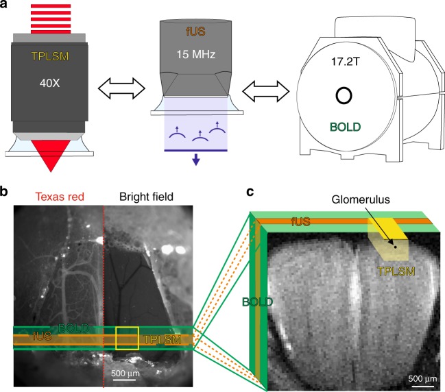
Fig. 1
A chronic mouse preparation compatible for imaging with TPLSM, fUS and BOLD-fMRI. a Experimental design: imaging the mouse brain with TPLSM, fUS and 17.2T BOLD-fMRI. b Dorsal view of a mouse olfactory...
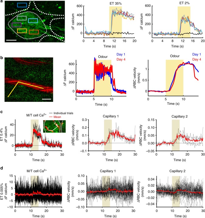
Fig. 2
Characterization of vascular responses to odour in mice implanted with a chronic PMP window. Mice expressing GCaMP6f under the Thy1 promoter were imaged with TPLSM. a Odour causes a homogenous elevati...
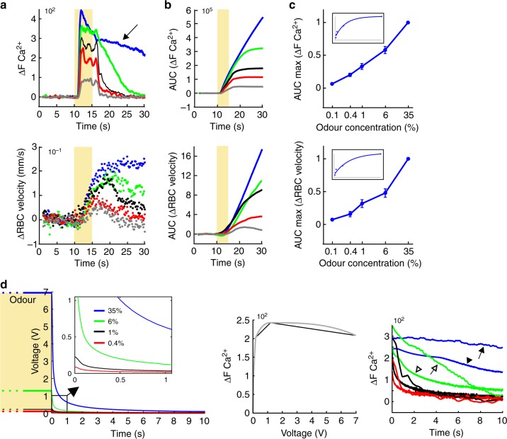
Fig. 3
Concentration dependency of neuronal and capillary blood flow responses to odour. a Neuronal (top) and RBC velocity (bottom) responses to odour at increasing concentration. Each trace is an average of...
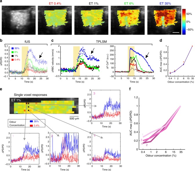
Fig. 4
Comparison of mesoscopic (fUS Power Doppler) and microscopic (TPLSM) responses to odour. a Spatial distribution u0394PD/PD voxel values at increasing concentrations of odour (ET). Maps are superimpose...
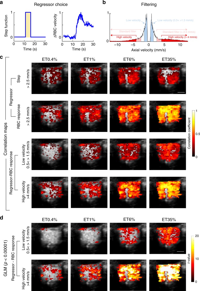
Fig. 5
Mapping vascular activation with fUS. a Shows regressor used for building fUS activation maps: Left: step function; Right: capillary RBC velocity response (here at 35% ET). b Spectrum of Doppler frequ...
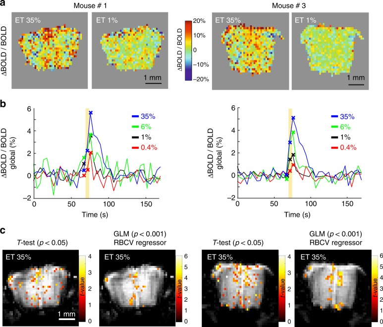
Fig. 6
BOLD-fMRI imaging of odour responses in the same mice. Left: mouse #1 (shown in Figs 4 and 5 ). Right: mouse #3 (shown in Fig. 3 ). a u0394BOLD/BOLD signal voxel map within the OB mask (no threshold w...
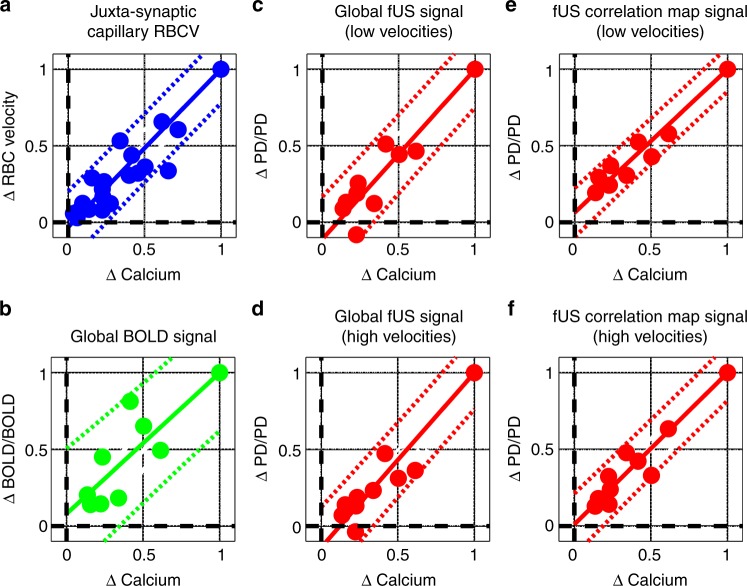
Fig. 7
Correlation of glomerular Ca 2+ with juxta-synaptic capillary and mesoscopic vascular signals. All vascular signals (both local and mesoscopic) are linearly related to glomerular Ca 2+ increases over ...
Figure images are served from the NIH/NLM PubMed Central Open Access Subset or Europe PMC; copyright remains with the publishers and authors.
💬 Discussion
0 commentsNo comments yet. Be the first to start a discussion!
Leave a Comment