Abstract
Biomaterial substrates can be engineered to present topographical signals to cells which, through interactions between the material and active components of the cell membrane, regulate key cellular processes and guide cell fate decisions. However, targeting mechanoresponsive elements that reside within the intracellular domain is a concept that has only recently emerged. Here, we show that mesoporous silicon nanoneedle arrays interact simultaneously with the cell membrane, cytoskeleton, and nucleus of primary human cells, generating distinct responses at each of these cellular compartments. Specifically, nanoneedles inhibit focal adhesion maturation at the membrane, reduce tension in the cytoskeleton, and lead to remodeling of the nuclear envelope at sites of impingement. The combined changes in actin cytoskeleton assembly, expression and segregation of the nuclear lamina, and localization of Yes-associated protein (YAP) correlate differently from what is canonically observed upon stimulation at the cell membrane, revealing that biophysical cues directed to the intracellular space can generate heretofore unobserved mechanosensory responses. These findings highlight the ability of nanoneedles to study and direct the phenotype of large cell populations simultaneously, through biophysical interactions with multiple mechanoresponsive components.
🔬 Techniques
🔭 Microscopes
💻 Software
✨ Fluorophores
🧪 Sample Preparation
🔬 Cell Lines
🏭 Microscope Brands
🧪 Reagent Suppliers
📷 Detectors
🔎 Objectives
💻 Software Details
🏛️ Research Organizations (ROR)
Affiliated research institutions:
📋 Methods
Fabrication of Nanoneedles Nanoneedles were fabricated according to our established protocol 28 , 35 on 100 mm diameter p-type doped Si wafers with 0.01 Ω·cm resistivity. A 1200 Å film of low stress silicon nitride was deposited by low-pressure chemical vapor deposition (Scottish Microelectronics Centre, UK). With an MA6 mask aligner (Suss Microtech, Germany), a pattern consisting of 0.6 μm dots with 2 μm pitch was transferred into a layer of NR9-250P photoresist (Futurrex, USA) spin-coated on the substrate. The pattern was transferred into the low stress nitride film with a 2 min 30 s reactive ion etching in CF 4 gas in an Oxford NGP80 (20 sccm, 200 W, 100 mTorr, Oxford Instruments, UK). The native oxide layer was stripped by soaking for 2 min in 10% v/v HF solution. The substrate was rapidly transferred in a 10% v/v HF solution of 0.02 M AgNO 3 and incubated for 2 min for electroless deposition of Ag nanoparticles. The substrate was transferred to a 10% v/v HF solution containing 0.12 M H 2 O 2 to undergo metal-assisted chemical etching for 8 min 30 s, forming porous pillar structures. The substrate was washed repeatedly in water and dried under N 2 stream. Reactive ion etching in SF 6 gas for 2 min 30 s (20 sccm, 100 mTorr, 250 W, Oxford NGP80) formed the final conical nN structures. The wafer was diced into 8 × 8 mm dies for subsequent use (DISCO Technologies, Japan). The typical nN had 3–4 μm length, a base diameter of 600 nm, and an apical diameter below 100 nm.
Preparation of Substrates
Samples were prepared as previously described. Substrate surfaces were activated using an oxygen plasma cleaner (10 min, Plasma Prep 5, Gala Instrumente, Germany) and then functionalized with 3-aminotriethoxysilane (APTES, Sigma-Aldrich, A3648) by liquid-phase conjugation in an ethanoic solution of 2% v/v APTES for 2 h. Following repeat washes in absolute ethanol (Sigma-Aldrich 32221), the nN arrays were dried under nitrogen. To generate fluorescent substrates, 0.0005% w/v 5 carboxytetramethylrhodamine N -succinimidyl ester (TAMRA, Sigma-Aldrich 53048) in phosphate-buffered saline (PBS) or 0.05 mg/mL fluorescein isothiocyanate isomer I (Sigma-Aldrich F7250) in PBS was conjugated to the APTES amine group with 2 h incubation followed by repeated washes with PBS and water. Nonfluorescent samples were sterilized under UV light for at least 20 min prior to cell experiments.
Show full methods section
Fabrication of Nanoneedles Nanoneedles were fabricated according to our established protocol 28 , 35 on 100 mm diameter p-type doped Si wafers with 0.01 Ω·cm resistivity. A 1200 Å film of low stress silicon nitride was deposited by low-pressure chemical vapor deposition (Scottish Microelectronics Centre, UK). With an MA6 mask aligner (Suss Microtech, Germany), a pattern consisting of 0.6 μm dots with 2 μm pitch was transferred into a layer of NR9-250P photoresist (Futurrex, USA) spin-coated on the substrate. The pattern was transferred into the low stress nitride film with a 2 min 30 s reactive ion etching in CF 4 gas in an Oxford NGP80 (20 sccm, 200 W, 100 mTorr, Oxford Instruments, UK). The native oxide layer was stripped by soaking for 2 min in 10% v/v HF solution. The substrate was rapidly transferred in a 10% v/v HF solution of 0.02 M AgNO 3 and incubated for 2 min for electroless deposition of Ag nanoparticles. The substrate was transferred to a 10% v/v HF solution containing 0.12 M H 2 O 2 to undergo metal-assisted chemical etching for 8 min 30 s, forming porous pillar structures. The substrate was washed repeatedly in water and dried under N 2 stream. Reactive ion etching in SF 6 gas for 2 min 30 s (20 sccm, 100 mTorr, 250 W, Oxford NGP80) formed the final conical nN structures. The wafer was diced into 8 × 8 mm dies for subsequent use (DISCO Technologies, Japan). The typical nN had 3–4 μm length, a base diameter of 600 nm, and an apical diameter below 100 nm.
Preparation of Substrates
Samples were prepared as previously described. Substrate surfaces were activated using an oxygen plasma cleaner (10 min, Plasma Prep 5, Gala Instrumente, Germany) and then functionalized with 3-aminotriethoxysilane (APTES, Sigma-Aldrich, A3648) by liquid-phase conjugation in an ethanoic solution of 2% v/v APTES for 2 h. Following repeat washes in absolute ethanol (Sigma-Aldrich 32221), the nN arrays were dried under nitrogen. To generate fluorescent substrates, 0.0005% w/v 5 carboxytetramethylrhodamine N -succinimidyl ester (TAMRA, Sigma-Aldrich 53048) in phosphate-buffered saline (PBS) or 0.05 mg/mL fluorescein isothiocyanate isomer I (Sigma-Aldrich F7250) in PBS was conjugated to the APTES amine group with 2 h incubation followed by repeated washes with PBS and water. Nonfluorescent samples were sterilized under UV light for at least 20 min prior to cell experiments.
Cell Culture
Human umbilical vein endothelial cells (HUVECs, Lonza) were expanded and seeded in endothelial growth medium-2 (EGM-2, Lonza) according to the manufacturer’s instructions. hMSCs were used between passages 4 and 6, and HUVECs were used between passages 5 and 10. For 6 h experiments, hMSCs were seeded at a density of 20 000 viable cells/cm 2 and HUVECs were seeded at a density of 30 000 viable cells/cm 2 , as determined by Trypan Blue exclusion. For 48 h experiments, hMSCs and HUVECs were seeded at different densities on flat and nN substrates to avoid confluent overgrowth. For hMSCs, cells were seeded at 2500 and 8375 cells/cm 2 for flat and nN substrates, respectively. For HUVECs, cells were seeded at 3000 and 12 500 cells/cm 2 for flat and nN substrates, respectively. Human mesenchymal stem cells (hMSCs, Lonza Ltd., Basel, Switzerland) were expanded in serum-free, chemically defined medium (MSCGM-CD) with supplements (TheraPEAK, Lonza), as per the manufacturer’s instructions. When ∼80% confluent, hMSCs were detached with 0.05% v/v trypsin-EDTA, reseeded at a density of 100–500 cell/cm 2 , and cultured for 7–14 days before reaching confluence. For interfacing with nN or flat substrates, hMSCs were seeded in minimum essential medium alpha (αMEM, Gibco ThermoFisher Scientific, Paisley, United Kingdom) with 10% v/v MSC-qualified fetal bovine serum (FBS, Gibco) and 1% v/v penicillin/streptomycin (P/S, Gibco). Latrunculin B, Lysophosphatidic Acid, and Staurosporine Treatment For treatment with Latrunculin B (LatB) or lysophosphaticid acid (LPA), cells were cultured for 5 h on flat or nN substrates, and then the medium was changed to include either dimethyl sulfoxide control (DMSO, Sigma-Aldrich, 1:10000), LatB (Sigma-Aldrich, 1:10000 in DMSO, 100 nM final concentration), or LPA (Santa Cruz Biotechnology, 1:500, 10 μm final concentration). Cells were then cultured for 1 h in the treated condition before end point experiments. For treatment with staurosporine, cells were cultured for the entire 6 h time course in either DMSO (1:10000) or staurosporine (Abcam 120056, in 1:10000 DMSO, final concentration 1 μM). After 6 h, cells were treated with fluorescent wheat germ agglutinin (WGA-555, ThermoFisher W32464 , 1:200) and CellEvent caspase-3/7 green detection reagent (ThermoFisher C10423 , 4 μM) in PBS with 5% v/v FBS for 30 min. Cells were then fixed with 3.7% w/v PFA, washed twice with PBS, and fluorescent images were captured to detect caspase activity.
Immunocytochemistry and Imaging
Cells were fixed in 3.7% w/v paraformaldehyde (PFA, Sigma-Aldrich) in PBS for 15 min at room temperature, then washed twice with PBS. For treatment with the cytoskeletal stabilization buffer (CSK, vinculin images), cells were incubated with CSK (10 mM PIPES, 50 mM NaCl, 3 mM MgCl 2 , 300 mM sucrose, 0.5% v/v Triton-X 100) for 1 min at 4 °C prior to fixation, following an established protocol. 53 Cells were then permeabilized with 0.25% v/v Triton X (Sigma-Aldich) for 10 min and blocked with 5% v/v donkey serum for 1–2 h. Primary antibodies were diluted in fresh 0.1% w/v bovine serum albumin (BSA, Sigma-Aldrich) in PBS and added to the cells overnight at 4 °C. Samples were then washed three times with PBS for 5 min before being incubated with secondary antibodies (1:500) in 0.1% w/v BSA for 60–90 min at room temperature; cells were then washed three more times with PBS for 5 min. Where applicable, samples were incubated with AlexaFluor-conjugated phalloidin (1:100–1:200 in 0.1% w/v BSA) for 1 h. All samples were counterstained with DAPI (1:1000, 1 μg/mL final concentration) for 5 min and stored upside down in Vectashield (H-1000 Vector Laboratories, Peterborough, United Kingdom) in glass-bottom chamber slides for imaging (Nunc, ThermoFisher Scientific). Antibody information is listed in Supplementary Table 1 . Confocal imaging was performed on a Leica SP5 microscope (Leica Microsystems, Wetzler, Germany), and z-stacks were collected with a 63× 1.4 NA oil-immersion objective lens at 700 nm step size and with a pixel size of 240 nm. Wide-field imaging was performed with an Axio Observer automated microscope (Carl Zeiss Meditec, Jena, Germany) with a 20× 0.8 NA dry objective and a pixel size of 240 nm imaged at 16 bits per pixel (Hamamatsu Flash4 sCMOS). 3D structured illumination microscopy (3D SIM) imaging was performed at room temperature with an Elyra PS.1 (Carl Zeiss). A 63× 1.4 NA oil-immersion objective lens was used, with three orientation angles of the excitation grid and five phases acquired for each image with a 110 nm z-step and a pixel size of 32 nm imaged at 16 bits per pixel on an Andor Zyla. SIM processing was performed with the SIM module of the Zen software package (Carl Zeiss), then TIF stacks of processed SIM data were exported. The SIM data sets were then turned into projection images using ImageJ software.
Live Cell Imaging
HUVECs were seeded in 35 mm plates for next day 70% confluency (100 k/cm 2 ). A ratio of 3:1 FuGENE HD transfection reagent (Promega, E2311)/DNA (Lifeact plasmid) with 1 μg of DNA was made up in Opti-MEM I reduced serum medium, GlutaMAX (Life Technologies, 51985-026), and 100 μL was added to the cells in EBM-2 basal medium (Lonza CC-3156) with 2% FBS. After 6 h, the medium was replaced with EGM. Forty-eight hours after transfection, cells were trypsinized and seeded on the nN in 24-well plates at a seeding density determined by the transfection efficiency. Following 2 h of incubation, to allow adherence of cell to the nN, the nN were inverted and placed down in an 8-well chamber slide containing EGM media and imaged on a wide-field Ti-E Eclipse microscope (Nikon-Minato, Japan) with a 20× 0.8 NA dry objective. The cells were imaged every 15 min for 2 h and 45 min with z-stacks of 5 μm range and 500 nm spacing.
Quantitative Real-Time Polymerase Chain
Reaction (qRT-PCR) Cells on nN or flat substrates were incubated with Trizol reagent (Life Technologies), mixed with chloroform (5:1 Trizol/chloroform), and separated by centrifugation (12 000 g , 15 min, 4 °C). The RNA contained within the aqueous phase was then isolated with RNeasy columns (Qiagen), according to the manufacturer’s instructions. cDNA was synthesized using a reverse transcription kit (Applied Biosystems, Life Technologies, product #4368814), and qRT-PCR was performed with a SYBR Green master mix (Applied Biosystems, Life Technologies, product #1179401K) with 2–5 ng of cDNA and 250–500 nM each of forward and reverse primers, using either a StepOne Plus or QuantStudio6 machine (Applied Biosystems). The qRT-PCR protocol was slightly different for the two machines. For the StepOne Plus, the protocol included the following: 95 °C for 20 s followed by 40 cycles of denaturation at 95 °C for 3 s and annealing at a temperature between 55 and 60 °C for 30 s. For the QuantStudio6, the protocol included the following: 95 °C for 20 s followed by 40 cycles of denaturation at 95 °C for 1 s and annealing at a temperature between 55 and 60 °C for 20 s. On both machines, a melt curve was subsequently performed in all reactions to ensure that a single amplicon was generated for each target gene. Cycles-to-threshold ( Ct ) values were automatically obtained using the ThermoFisher Scientific Cloud Software for qPCR file processing ( https://www.thermofisher.com/uk/en/home/cloud.html ). These values were subsequently exported to an Excel file and manually processed to generate fold change expression values. The expression of each gene of interest was normalized to the geometric mean 54 of the expression of at least two housekeeping genes ( PPIA , RPL13A , and/or HPRT1 ), generating the Δ C ( t ) value, and expression of 2 –ΔΔ C ( t ) relative to the flat control for each cell type, and N ≥ 3 experimental replicates are reported. Statistical analysis information is listed in the relevant section below. Custom primers were purchased from Invitrogen and tested for specificity prior to use. Sequences are listed in Supplementary Table 2.
Extraction of Cell Lysates and Western Blotting
Medium from cells on nN or flat substrates was gently aspirated, and cells were rinsed two times with ice cold PBS. Cell lysate from 8 chips were extracted in 300 μL of cell lysate buffer (4 M urea, 150 mM NaCl, PhosSTOP (Roche), and complete EDTA-free protease inhibitor cocktail (Roche)) by scraping on ice. Lysates were sonicated using an immersion probe for 10 s pulse at 200 W. Insoluble protein was removed by centrifuging at 15 000 g for 10 min at 4 °C. Protein was quantified using Qubit protein assay ( Q33211 , Thermo) and Qubit fluorometric quantification instrument (Thermo). Protein samples were prepared with 4× sample buffer containing β-mercaptoethanol in a ratio of 3:1 and heated at 80 °C for 5 min. SDS-PAGE electrophoresis was conducted using TGS running buffer (Bio-Rad) for 45 min at 100 V. Gel transfer was conducted using Transblot-turbo (Biorad). Blots were probed with primary mouse anti-human vinculin (Abcam ab18058, 1:1000) and secondary (Li-Cor IR 680, 1:1000) antibodies in iBind fluorescent solution (SLF1019, Thermo) using the respective iBind Flex western device. Blots were analyzed for intensity of fluorescent band using a Li-Cor Odyssey imaging system.
Scanning Electron Microscopy
Cells on nN or flat substrates were fixed in 2.5% v/v glutaraldehyde solution (Sigma) for 1 h in PBS at room temperature and then washed three times in PBS. PBS buffer was substituted with 0.1 M sodium cacodylate buffer (Electron Microscopy Sciences, USA), and cells were washed twice for 5 min. Cells were postfixed in 1% v/v osmium tetroxide for 1 h in 0.1 M sodium cacodylate buffer and subsequently washed with distilled water two times for 5 min. Samples were dehydrated in a series of ethanol dilutions (20, 30, 50, 70, 80, 90% v/v ethanol in water), treated with 100% ethanol four times for 5 min, after which they were treated with hexamethyldisilazane for 5 min and air-dried. Samples were mounted and sputtered with 10 nm of chromium (Q150, Quorum) and imaged using Sigma300 (Zeiss) scanning electron microscope with a working distance of 10 mm and an accelerating voltage of 5 keV. Quantifying Actin Stress Fibers Actin stress fibers were quantified from confocal images. To highlight stress fibers, the actin channel was filtered by performing convolution with a 6 by 10 kernel with the central two columns containing a positive value and outer four columns containing a negative value. Convolution was performed with orientations of the kernel at 3° intervals between 0 and 180°, and the maximum value for each pixel over 60 orientations was then selected. Other kernel shapes and orientation regimes were tested; however, this choice emphasized stress fibers most effectively, as judged by visual inspection ( Figure S2 ). Thresholding was then performed on these images, and the subsequent binary mask appeared to match stress fibers well. Regions below 100 pixels in size were removed as these were largely noise. Quantifying Focal Adhesion Density To determine the focal adhesion density, the number of focal adhesion regions in the image, divided by the image area covered by actin (determined by a similar threshold operation to blurred actin image) was calculated. Significance was determined by pairwise t test between 10 analyzed fields of view taken over two experimental repeats.
Quantitative Cell Morphology Analysis
Quantification of cell and protrusions morphology was performed on tiled wide-field microscopy images using the MATLAB image analysis toolbox. Background correction was performed by negating the image with itself, following very large Gaussian blur. Marker controlled watershed segmentation was then performed on DAPI channel to identify nuclei. Nuclei touching the border, or below a threshold intensity, were filtered. To identify the cell cytoplasm, thresholding was performed on the actin channel to identify the image region containing cells. Watershed on the actin channel resulted in extensive mis-segmentation, thus utilizing nuclei as markers, and the actin containing image region as the boundary, marker-controlled watershed segmentation was performed on the YAP channel. This resulted in effective detection of cell boundaries with the substrate and with other cells. Cells with mean actin intensity similar to background were filtered out, as were those touching the border.
Feature Extraction
Features describing cell and protrusion morphology were extracted from cell and nuclei segments. For intensity and texture properties, the original images were used, without background correction; however, images were log transformed, and subsequently the 10th percentile intensity was deducted to align background intensity to zero, thus reducing technical intensity variations between replicates. Protrusion regions are defined by applying a large erosion and dilation operation to the whole cell segment. This generated a highly rounded core, region of cytoplasm not in this core are defined as protrusions. A list of the features extracted for linear discriminant analysis is given below. Morphology (except Actin Channel Intensity) Cell area Cell major axis length: length of the equivalent ellipse based upon second order moments Cell minor axis length: width of the equivalent ellipse Cell eccentricity: eccentricity of the equivalent ellipse Cell extent: proportion of pixels within the bounding box Cell solidity: proportion of pixels in the convex Cell perimeter: perimeter length of cell segment Cell roundness: defined as Cell channel intensity: mean actin intensity: not included for LDA Number of protrusions per cell Mean protrusion area per cell Max protrusion area per cell Total protrusion area per cell Mean length of protrusions per cell (major axis length of equivalent ellipse) Max length of protrusion per cell Total length of protrusions per cell Mean width of protrusion per cell (minor axis length of equivalent ellipse) Max width of protrusion per cell Total width of protrusion per cell Mean extent of protrusions per cell, defined as length from nuclei center of mass to furthest point in protrusion region minus length from nuclei center of mass to nearest point in protrusion region. Max extent of protrusion per cell Total extent of protrusion per cell Actin Texture Calculated from Gray Level Co-occurrence Matrix (GLCM) Contrast: variance between neighboring pixels Correlation: correlation between neighboring pixels Energy: angular second moment of the image Homogeneity: a measure of how sharp are gradients within the image Additional Features Nuclear centroid X position Nuclear centroid Y position Nuclear orientation angle of equivalent ellipse Cell orientation angle of equivalent ellipse Mean intensity of central actin (following erosion of cytoplasmic segment mask) Mean intensity of cortical actin (mask of cytoplasmic ring region that is eroded to form central region) Protrusion Features Index of cell protrusion. This links protrusions to the unique cell ID in the corresponding single cell data file. Protrusion area Length of protrusion (major axis length of equivalent ellipse) Width of protrusion (minor axis length of equivalent ellipse) Protrusion orientation angle of equivalent ellipse Extent, defined as length from nuclei center of mass to furthest point in protrusion region minus length from nuclei center of mass to nearest point in protrusion region Linear Discriminant Analysis LDA between flat substrate and nN was performed on cells pooled over 3 experimental repeats for HUVEC and hMSC cells, with two technical repeats for two experiments, and one technical replicate for one experiment. Each cell type was analyzed independently, where cells were labeled as “Flat” or “nN” and the features described above were extracted for all cells. R 2 values for HUVEC and hMSC cells were 0.286 and 0.343, respectively; p < 0.001 in both cases. Also, LDA applied to data following random permutation of class labels led to insignificant separation. These R 2 values correspond to 75 and 78% correct substrate classification of HUVEC and hMSC cells, respectively. The box plot in Figure 1 shows a random sample of 900 cells from each group. This analysis was conducted with the Scikit-Learn module for Python. 55 YAP Localization Analysis YAP intensities and localization were calculated following cell and nuclei segmentation as described above. Three features on YAP localization were recorded: Nuclear YAP intensity: taken as the median of the nuclear YAP intensities Cytoplasmic YAP intensity: the cytoplasmic segments was eroded by a fixed width (10px), such that pixels bordering the substrate and other cell were not included, subsequently the median YAP intensity from this region was taken. Log nuclear to cytoplasmic YAP ratio YAP nuclear to cytoplasmic localization changes both in wild-type and following drug and DMSO treatment were recorded from a pooled random sample of 180 cells taken over two experimental repeats, with two technical repeats per experiment. Significance of differences was calculated using a pair wise t test between single cell populations.
Focal Adhesion Quantification
To identify focal adhesions, a similar approach to actin stress fiber identification was employed. Confocal images of cells treated with CSK and then stained for vinculin were used for image analysis. Vinculin channel images were filtered by performing convolution with a 5 by 6 kernel with the central two columns containing a positive value and outer two columns containing a negative value. Convolution was performed with orientations of the kernel at 10° intervals between 0 and 90°, the maximum value for each pixel over the 9 orientations was then selected. Following thresholding similar to actin bundle quantification ( Figure S2 ), regions below 10 pixels in size were removed as these were largely noise. Again, to determine the focal adhesion density, the number of focal adhesion regions in the image divided by the image area covered by actin (determined by a similar threshold operation) was calculated. Significance was determined by pairwise t test between 10 analyzed fields of view taken over two experimental repeats. Quantification of Lamin Signal In Figure 4 E–G, single cells were isolated from cropped confocal z-stack images for analysis using ImageJ software (National Institutes of Health, Bethesda, MD, USA). A line was drawn in the x – y plane along a row of nN interacting with the nuclear envelope, and a reslice image was created (reslice shown in Figure 4 I). Reslice line width was 25 pixels for Figure 4 F and 20 pixels for Figure 4 G. From the reslice images, one of two quantifications was performed. For data in Figure 4 F, a line of 20 pixel width was created in the reslice image and hand-drawn along the base of the nuclear envelope and up the entire z-height of each individual nN. Along this line, the signal for lamin A and lamin B channels were recorded (test line). In another area of the nuclear envelope where nN were not interacting ( i.e. , top nuclear envelope or space between nN interfacing), an additional line of 20 pixel width was drawn, and the lamin A and lamin B signal values over this line were averaged as a normalization factor for that specific reslice image (normalization line). Then, all values recorded from the test line were normalized to the respective average calculated from the normalization line, providing a fold change measurement for each lamin channel within that particular reslice image. To obtain the data in Figure 4 G, reslice images were prepared in the same way, and two additional lines were prepared for measurement of signal within the reslice image. Two identical lines of 20 pixel width were drawn in the y -direction (that is, perpendicular to the nN height). One line was placed in the middle of the nN z-height (middle line) and an identical line was z-shifted to the top of the nN z-height (top line), and signals for nN, lamin A, and lamin B channels were recorded. Similar to above, a normalization line was also recorded from an area within the reslice along a 20 pixel width line where nN were not interacting. The troughs within the nN signal were detected from the inflection points around local maxima of the nN signal from the middle line. Lamin A and/or lamin B signals were then integrated from trough-to-trough distances for the middle and top lines. This analysis was performed because measurement of lamin A or B signal at specific points along the nN width in the original reslice image did not reveal the accumulation of the protein signal around the nN in the y -direction. Integrated values were subsequently normalized to the respective average values calculated from the normalization line, and the ratio of integrated lamin A/B at the nN middle and top is reported. In Figure S11 , the integrated values for lamin A or B at the middle or top were normalized and reported.
Statistical Analysis
Statistics on biochemical data were performed with GraphPad Prism software (La Jolla, CA, USA). When comparing two groups, a Student’s unpaired t test was performed. When comparing more than two groups, a one-way analysis of variance (ANOVA) was performed, followed by pairwise comparisons via Bonferroni’s multiple comparison test. For the comparison of lamin A/B ratios in Figure 4 , a nonlinear exponential curve was fit to the data set, and the best-fit values are reported. For image analysis, MatLab (Mathworks, Cambridge, UK) was used to analyze data and prepare charts. For qPCR analysis, three to four experimental replicates were performed, with at least two biological replicates within each experiment. For each experimental replicate, the expression of the gene of interest (GOI) was normalized to the geometric mean of at least two housekeeping genes (HKGs) following previous methods, 56 which generated the Δ Ct value. For each cell type, the average was calculated for the normalized GOI expression on flat samples, and expression of all groups was then normalized to these values. This resulted in an expression value equal to 1 for HUVEC or hMSC flat samples but carried a nonzero standard deviation that reflected the intraexperimental heterogeneity of biological replicates. In order to propagate this error, the relative standard deviation (RSD) was calculated for all groups of interest, where where N is the number of experimental replicates ( N = 3–4) and SD_expRep represents the standard deviation of the normalized expression for each group within each experimental replicate. This approach allowed for the variability within each experiment to be propagated. Of note, for lamin A and lamin B gene expression in Figure 4 , the expression of all groups was normalized to HUVEC flat so that cell type-specific differences in lamin signal could be observed. For Figure S13A–D , Δ Ct values for each GOI were compared as a ratio and were not normalized to the expression of the flat control cells ( i.e. , ANKRD1/LMNA describes Δ Ct _ ANKRD1 /Δ Ct _ LMNA ). For all box plots, the 25th and 75th quartiles are represented, the line is the median, and the whiskers extend to the minimum and maximum data points, unless the point is a statistical outlier (and is therefore shown in red). For all experiments, p < 0.05 was considered significant.
Data Availability
Raw data are available upon request from rdm-enquiries@imperial.ac.uk .
Supplementary Material nn8b06998_si_001.pdf nn8b06998_si_002.avi nn8b06998_si_003.avi nn8b06998_si_004.avi nn8b06998_si_005.avi
📊 Figures
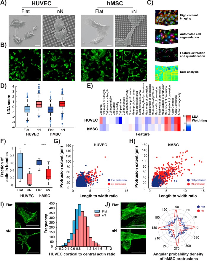
Figure 1
Nanoneedle interaction with HUVECs andnhMSCs reduces actin bundlingnand enhances actin-rich protrusions. (A) SEM images show direct interactionnbetween cells and nN 6 h postseeding. Scale bars = 10 u0...
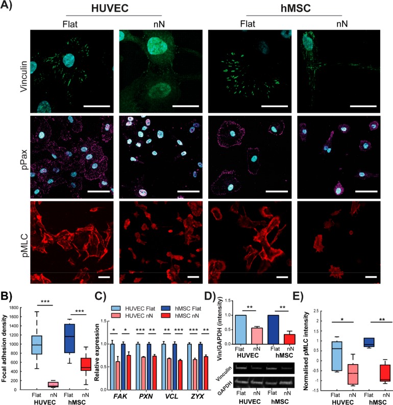
Figure 2
Nanoneedlesninhibit focal adhesion formation and generation ofnintracellular tension. (A) Confocal maximum projection images 6 hnpostseeding. On flat substrates, dense vinculin staining is observednin...
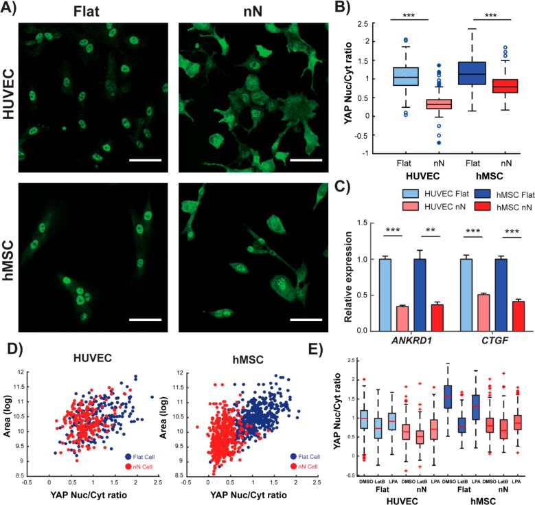
Figure 3
Nanoneedles reduce YAPnactivity and lessen the correlation betweennYAP activation and cell spreading. (A) Confocal microscopy shows nuclearnYAP protein localization on flat substrates and cytosolic lo...
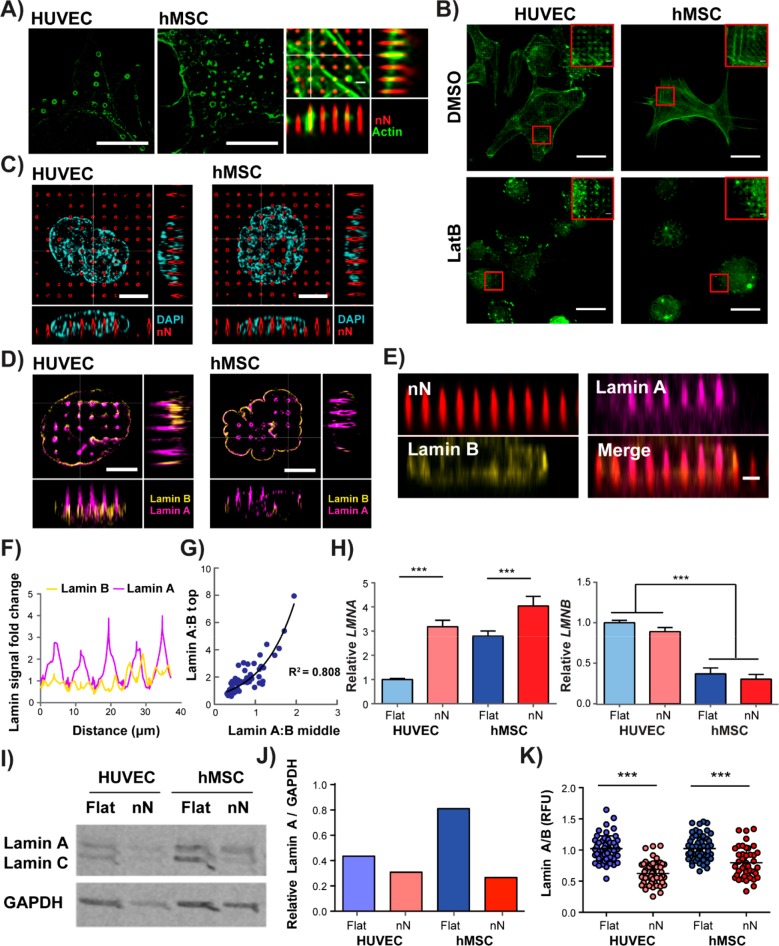
Figure 4
Nanoneedles interactnwith mechanoresponsive organelles. (A) Polymerizednactin rings form at sites of nN interaction with both HUVECs and hMSCs,n(HUVEC: structured illumination microscopy (SIM), single...
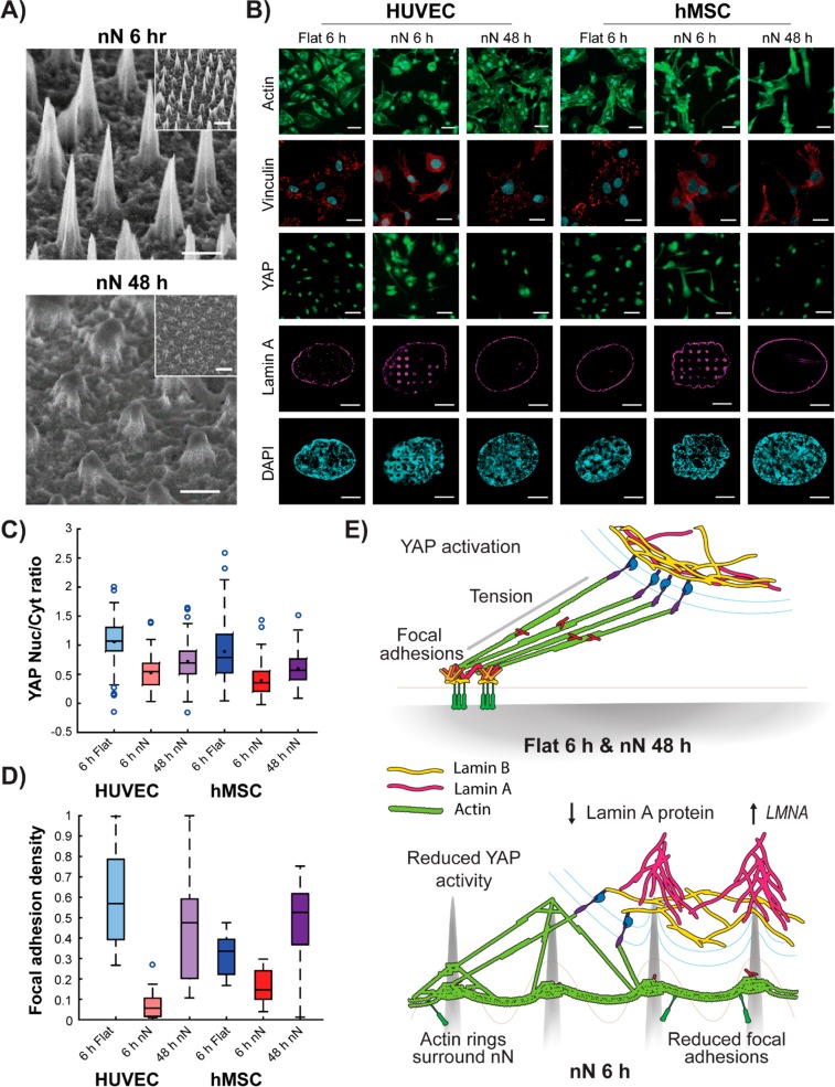
Figure 5
Nanoneedle degradation recovers mechanoresponsive cellnbehaviors.n(A) SEM images show nN degradation after 48 h in culture. Scale barsn= 1 u03bcm, 2 u03bcm inset. (B) Cell phenotype is restored onndeg...
Figure images are served from the NIH/NLM PubMed Central Open Access Subset or Europe PMC; copyright remains with the publishers and authors.
💬 Discussion
0 commentsNo comments yet. Be the first to start a discussion!
Leave a Comment