Abstract
Diverse cellular signaling events, including B cell receptor (BCR) activation, are hypothesized to be facilitated by domains enriched in specific plasma membrane lipids and proteins that resemble liquid-ordered phase-separated domains in model membranes. This concept remains controversial and lacks direct experimental support in intact cells. Here, we visualize ordered and disordered domains in mouse B lymphoma cell membranes using super-resolution fluorescence localization microscopy, demonstrate that clustered BCR resides within ordered phase-like domains capable of sorting key regulators of BCR activation, and present a minimal, predictive model where clustering receptors leads to their collective activation by stabilizing an extended ordered domain. These results provide evidence for the role of membrane domains in BCR signaling and a plausible mechanism of BCR activation via receptor clustering that could be generalized to other signaling pathways. Overall, these studies demonstrate that lipid mediated forces can bias biochemical networks in ways that broadly impact signal transduction.
🔬 Techniques
🔭 Microscopes
💻 Software
✨ Fluorophores
🧪 Sample Preparation
🔬 Cell Lines
🏭 Microscope Brands
🧪 Reagent Suppliers
📷 Detectors
🎨 Filters
💻 Software Details
📋 Protocols
💾 Data Repositories
🏷️ Research Resource Identifiers (RRIDs)
Verified research resources used in this paper:
🏛️ Research Organizations (ROR)
Affiliated research institutions:
📋 Methods
Materials and methods f(Ab) 1 and antibody modification f(Ab) 1 fragment goat antibody to mouse IgM, µ chain specific (Jackson ImmunoResearch, West Grove, PA; RRID: AB_2338477 ) was simultaneously chemically modified with Atto 655 NHS ester (Sigma, St. Louis, MO) and biotin-X, SSE, 6-((Biotinoyl)Amino)Hexanoic Acid, Sulfosuccinimidyl Ester, Sodium Salt (Sulfo-NHS-LC-Biotin) (Invitrogen, Grand Island, NY). Modifications were carried out in aqueous solution buffered by 0.01 M NaH 2 PO 4 with 0.01 M NaH 2 CO 3 , pH 8.2 for thirty minutes at room temperature. Reaction products were separated by gel filtration on Illustra NAP-5 columns (GE Healthcare, Piscataway, New Jersey) to remove unbound dye from labeled protein. CTxB (Invitrogen) was biotylated and conjugated to Atto 655 in-house via similar methods, and both CTxB and f(Ab) 1 conjugation was also described previously ( Stone and Veatch, 2015 ). f(Ab) 1 was also conjugated to silicon rhodamine (SiR) dye (Spirochrome, Switzerland) in conjunction with biotin by similar methods. Streptavidin (Invitrogen) and anti-mouse IgG2b (Jackson ImmunoResearch; RRID: AB_2338463 ) were also conjugated to either Alexa 532 (Invitrogen) or Atto 655 by similar methods. CTxB that was only biotinylated (without Atto 655 conjugation) was purchased directly from Invitrogen. The commonly used STORM dye Alexa 647 was not used in most cases due to issues associated with the presence of near-red fluorophores present in reactive dye stocks ( Stone and Veatch, 2014 ). DNA constructs Lyn-eGFP, PM-eGFP, and eGFP-GG plasmids ( Pyenta et al., 2001 ) were a generous gift from Barbra Baird and David Holowka (Cornell University, Ithaca, NY) and were cloned using standard techniques to replace eGFP with mEos3.2. Plasmid DNA encoding mEos3.2 protein and YFP-TM anchor sequences were gifts from Akira Ono (University of Michigan, Ann Arbor, MI). The YFP and mEos3.2 tagged constructs used here are in Clontech N1 plasmid vector background (Clontech, Mountain View, CA). The clathrinHC-GFP and clathrinHC-mEos3.1 constructs ( Sochacki et al., 2014 ) were gifts from Justin Taraska (National Heart, Lung, and Blood Institute, NIH, Bethesda, MD). We also cloned the CD45 transmembrane domain (termed CD45 tm ) with a small number of flanking amino acids de novo from the amino acid sequence for mouse CD45 isoform 1, UniParc identifier P06800 –1. We included the HA membrane-targeting signal sequence and a FLAG tag ( Guan et al., 1992 ) upstream of the construct on the N terminus to allow for efficient plasma membrane delivery and detection, respectively. The signal sequence is cleaved from the construct in the ER prior to trafficking to the plasma membrane. The CD45 transmembrane domain was cloned into the HA-FLAG tag plasmid using standard techniques. Amino Acid sequence of CD45 tm insert with upstream HA-FLAG tag, where the signal sequence is shown in italics and the FLAG tag is shown in bold: N terminus- MKTIIALSYIFCLVFA DYKDDDDA NESTNFNAKALIIFLVFLIIVTSIALLVVLYKIYDLRKKR-C terminus Cells and transfection CH27 cells (RRID: CVCL_7178 ), a mouse B cell lymphoma-derived cell line, was used as a model system for B lymphocyte signaling through the BCR ( Haughton et al., 1986 ). Cells were acquired from Neetu Gupta (Cleveland Clinic), and cell line identity was authenticated using several criteria. Surface expression of mouse IgM, which is a specific marker of mouse B lymphocytes, was confirmed through specific labeling with goat anti-mouse IgM f(ab) 1 fluorescent conjugates. Cell morphology was typical for the B lymphoma cell type. Growth rates were monitored for consistency over time and cells were not kept in passage for longer than 60 days. Cultures tested negative for mycoplasma contamination. CH27s do not appear on the list of commonly mis-identified cell lines maintained by the International Cell Line Authentication Committee. Cells were maintained in culture as described previously ( Stone and Veatch, 2015 ). CH27 cells were transiently transfected by Lonza Nucleofector electroporation (Lonza, Basel, Switzerland) with electroporation program CA-137. Generally, 700,000 CH27 cells were transfected with 1 µg plasmid DNA, except for Lyn where 500,000 cells were transfected with 0.7 µg plasmid DNA to avoid cell death. Cells were grown overnight on glass bottom wells (MatTek Corporation, Ashland, MA) at 200,000 per well. A subset of CH27 cells adhere spontaneously to glass bottom wells via an unknown mechanism but adhesion is not, in our experience, potentiated by first coating wells with fibronectin. For GG expression, cells were grown overnight in flasks, harvested and spun down, washed by pelleting and re-suspending three times in media, and then plated on the same day as labeling and fixation to minimize coverslip-bound mEos3.2-GG because this construct is secreted from cells. For cholesterol depletion and addition, cells were incubated for 15 min at 37°C with indicated concentrations of MβCD or cholesterol loaded MβCD (Sigma) freshly dissolved in Balanced Salt Solution (BSS: 135 mM NaCl, 1 mM MgCl 2 , 1.8 mM CaCl 2 , 5.6 mM glucose, 20 mM HEPES, pH 7.4). Cells were chemically fixed with 4% paraformaldehyde and 0.1% glutaraldehyde in PBS buffer or 2% paraformaldehyde and 0.15% glutaraldehyde in half-strength PBS for 10 min at room temperature unless otherwise indicated, and fix was quenched by washing with 5 mg/mL BSA. Primary B lymphocytes were purified from a C57BL/6 mouse (Jackson Laboratories; RRID: IMSR_JAX:000664 ) using a standard negative selection procedure. All experiments were performed in compliance with federal laws and institutional guidelines as approved by the University of Michigan Committee on Use and Care of Animals. Briefly, one mouse was sacrificed using CO 2 asphyxiation. Spleen and lymph nodes were harvested in the presence of DNase I and filtered through a 70 µm strainer. Cells were pelleted and resuspended in DMEM with 2% FBS, 10 mM HEPES, 50 IU/mL penicillin, 50 µg/mL streptomycin, and 0.2 mg/mL DNAse I. 5 µg/mL CD11c (clone N418, Biolegend; RRID: AB_313772 ) and 5 µg/mL CD43 (clone S7, BD Biosciences; RRID: AB_2255226 ) biotinylated antibodies were added to cells for 30 min on ice prior to red blood cell lysis with RBC lysis buffer (0.14 M NH 4 Cl and 0.017 M Tris, pH 7.2) and washing by pelleting. Remaining cells were incubated with streptavidin MACS beads (Miltenyi Biotec) for 20 min on ice and non-B cells were removed using an Automacs (Miltenyi Biotec) on the DEPLETES protocol. Primary B cells were then put into a buffer recommended by Lonza: RPMI 1640 supplemented with 10% FCS, 2 mM glutamine, 50 µM 2-mercaptoethanol, and 50 µg/mL LPS for 24 hr. Electroporation was accomplished with the P4 Primary Nucleofector solution with electroporation program DI-100 (Lonza) using 600,000 cells with 0.6 µg plasmid DNA in each well. Cells were grown overnight in flasks, spun down and washed extensively in cell media, and then plated onto fibronectin plates for 2 hr prior to labeling with f(Ab) 1 biotin Atto 655, clustering with streptavidin, and fixation as described above. RBL-2H3 cells (ATCC CRL-2256; RRID: CVCL_0591 ), a rat basophilic leukemia-derived cell line, were obtained from Barbara Baird and David Holowka (Cornell University). Cell identity was authenticated by expression of the high-affinity receptor for IgE, FcεRI, which was confirmed by specific binding of fluorescent IgE conjugates to the surface of cells. Cells were checked for characteristic morphology ( Siraganian et al., 1982 ), growth rates were monitored for consistency over time, and cells were not kept in passage for longer than 90 days. Cultures tested negative for mycoplasma contamination. RBL-2H3 cells do not appear on the list of commonly mis-identified cell lines maintained by the International Cell Line Authentication Committee. RBL-2H3 cells were maintained in minimum essential medium with L-glutamine and phenol red with 20% fetal bovine serum and 0.1% gentamycin at 37°C in 5% CO 2 , as described previously ( Gosse et al., 2005 ). RBL-2H3 cells were transiently transfected with membrane anchor probes using the protocol described above for CH27 cells, with electroporation program DS-138. HeLa cells were obtained from Akira Ono (University of Michigan) and maintained in high-glucose (4 mg/ml) Dulbecco's Modified Eagle Medium with 5% fetal bovine serum and 1% pen strep at 37°C in 5% CO 2 . HeLa cells were only used for experiments to demonstrate properties of the analytical methods used ( Figure 6 ), where cell identity was not pivotal to the interpretation of results. Cells had morphology and adhesive qualities common to this cell line but were not subjected to additional authentication. HeLa cells were transiently transfected using the protocol described above for CH27 cells, with electroporation program CN-114. 10.7554/eLife.19891.042 Figure 6. Our cross-correlation methodology applied to doubly labeled clathrin. ( a ) Two-color super-resolution image of a HeLa cell expressing two distinct labeled clathrin heavy chain constructs is shown. Clathrin heavy chains associate strongly in clathrin coated pits, and thus serve as an example of highly correlated co-clustered objects. Individual clathrin coated pits are shown below in the smaller images. Scalebar in large image is 5 µm, scale-bars in small images are 200 nm. ( b ) Zoom in of cyan box shown in large image, where position of points are plotted around an arbitrarily chosen central magenta localization. Dotted lines show the spatial bins used for calculating the cross-correlation function, where the number of green localizations within each bin are counted. In the complete cross-correlation these counts would also be summed over all magenta localizations. ( c ) Raw histograms of interparticle distances containing all pairs of particles localized within this cell. The red line shows the expected number of pairs in each spatial bin given a random distribution of both magenta and green localizations. The raw histogram is normalized by this curve to yield c(r). ( d ) Cross-correlation derived from localizations within this cell. Magnitude of the correlation indicates fold increase of pairs detected at the specified inter-particle distance compared to a random distribution. The expected value of the cross-correlation given a random co-distribution is equal to one due to the normalization. Error bounds shown are dC 2 (r) and are estimated from the statistics and resolution of the image as defined in Equation 3 . DOI: http://dx.doi.org/10.7554/eLife.19891.042 10.7554/eLife.19891.043 Figure 6—figure supplement 1. The cross-correlation function detects deviations in the co-distribution of localizations from random. Four simulations of two-color localization distributions are shown, where the spatial distribution of the localization is given by the labels in the top left of the images. For clustered distributions, particles are randomly placed within non-overlapping circular areas. For co-clustered, both green and magenta localizations are placed within the same circular areas. Cross-correlation functions calculated from simulated distributions are shown at right. Only co-clustered objects yield a cross-correlations that is significantly different from a random distribution. Clustering one object and leaving the other randomly distributed or clustering both objects but maintaining a random co-distribution yields distributions of interparticle distances that are not significantly different than a random co-distribution of both localizations. Scale bars are 100 nm. DOI: http://dx.doi.org/10.7554/eLife.19891.043 10.7554/eLife.19891.044 Figure 6—figure supplement 2. The amplitude of the cross-correlation reflects differences in enrichment magnitude and interaction strength. Example cells from three different experiments are shown to illustrate the range of values the cross-correlation function can take for various types of interactions. ( a ) An example of a strong enrichment is shown for phosphotyrosine (pY) and BCR. Nearly every BCR cluster is colocalized with pY localizations, and little pY is observed outside BCR clusters. ( b ) Lyn transiently binds to phosphorylated ITAMs within BCR clusters but is also present outside of clusters, leading to a reduced magnitude of the correlation function. ( c ) PM is weakly enriched in BCR clusters and a large fraction of PM is found outside of BCR clusters, however PM is more colocalized than expected from a random distribution when the whole cell is analyzed. In whole-cell images (top), scale bars are 5 µm. Boxed regions shown in whole-cell images are enlarged below (middle) and the number of localizations in each pixel is given by the colorbars. Scale bars in enlarged regions are 100 nm. DOI: http://dx.doi.org/10.7554/eLife.19891.044 10.7554/eLife.19891.045 Figure 6—figure supplement 3. Cross-correlations detect co-clustering even when there is a low surface density of labeled molecules. An Ising model containing kinase (green) and clustered receptors (magenta) is used to demonstrate how the surface density of labeled proteins impacts correlation functions. (top) Representative histograms indicating simulated positions of kinase and receptors, with each pixel corresponding to 16 nm × 16 nm area. The average surface density per µm 2 is shown. (middle) The same image as above but blurred by a Gaussian function mimicking the localization precision. All scale bars are 100 nm. (bottom) Averaged cross-correlation functions for the conditions represented above. The black curve shows an average over 1000 samplings of the same distribution with the average surface density indicated for both kinase and receptor. The colored lines show averages over 100 samplings. If there are roughly 100 receptor clusters per cell, then these curves represent the expected cell-to-cell variation. Most experiments have mEos3.2 surface expression between 1–20 per µm 2 so are expected to most closely mimic the situation on the far right. Note that even when surface densities are low, the average correlation function remains unchanged beyond differences in signal to noise. DOI: http://dx.doi.org/10.7554/eLife.19891.045 10.7554/eLife.19891.046 Figure 6—figure supplement 4. Membrane topology gives rise to long-range structure in cross-correlations, but can be removed by careful selection of regions of interest (ROI). ( a ) Reconstructed super-resolution image of a CH27 B cell in which part of the cell has detached from the coverslip surface leading to a reduction in localizations in the center of the cell, which is imaged in total internal reflection. Two different regions of interests are shown, with the excluded regions lightened for contrast. Scale bars are 5 µm. ( b ) Cross-correlation functions tabulated using the two ROIs shown in a. The loose ROI produces a C(r) that is correlated and decays slowly with radius. This is largely a reflection of the topology of the ventral membrane, which contains large regions where both probes are excluded due to membrane detachment. This correlation is removed by selecting a ROI which only includes flat regions. ( c ) ROI generation is performed by users and has the potential to introduce bias into the analysis. 19 cells comprising different labeling and treatment conditions were randomly viewed by users that lacked knowledge of the specific identity of each cell. The three users tended to define masks that yielded correlation functions with similar amplitudes from single cells. ( d ) Average cross-correlation curves corresponding to the 19 cells shown in d, with errorbars indicating the SEM between cells for each user. These results overlap within error bounds suggesting that arbitrary user decisions regarding ROI placement do not significantly impact this result. DOI: http://dx.doi.org/10.7554/eLife.19891.046 10.7554/eLife.19891.047 Figure 6—figure supplement 5. Estimation of the variance associated with a cross-correlation measured on a single super-resolution fluorescence localization image. Simulations containing randomly distributed green and magenta points are used to identify the sources of error typically found in cross-correlations tabulated from images acquired using super-resolution localization microscopy. Here, labeled molecules are distributed randomly as shown in ( a ). When the localization precision (30 nm) is on the order of the pixel size (25 nm), then it acts to blur the image of molecular centers ( b ). The smooth blurred image represents a fully sampled PSF. In real localization microscopy images, single labeled molecules are typically localized multiple times, but not often enough to fully sample the super-resolved PSF. Instead the distribution represented by the blurred image is under-sampled. The smooth shape of the PSF is still evident when each PSF is sampled many times (c), but images appear more pixelated as this sampling is reduced (d). All of these factors impact the statistics of measured correlation functions. For all conditions indicated, the top panel shows a representative simulation snapshot for the condition indicated (scale-bar = 500 nm) and the two dimensional cross-correlation, C(r, θ), tabulated from this representative image. The next lower panel shows C(r, ) obtained by averaging C(r, θ) over angles (red squares), as well as , the correlation function obtained by averaging over 100 simulation replicates (black circles). Error bars on these curves are either determined from the angular average as described in the main text (red squares, dC(r, )), or by taking the SEM over 100 simulation replicates to obtain d (black circles). The bottom panels show how the square root of the variance (dC(r)) depends on radius for the conditions indicated. Black circular points show (d). Red squares show the dC(r, ) error averaged over the 100 replicates . The dC 1 (r) and dC 2 (r) points are corrections to dC(r, ) and are calculated as described in Methods. ( a ) dC(r, ) is a good estimate of d in simulations where the localization precision is much less than the pixel size and when there is good sampling of the super-resolved PSF. ( b ) dC(r, ) under-estimates d when labeled objects are detected with 30 nm localization precision but when these super-resolved PSFs are fully sampled. This under-estimate can be corrected using the dC 1 (r) described in Equation 2 of Methods. ( c ) dC 1 (r) is sufficient when labeled objects have 30 nm resolution and their super-resolved PSF is well sampled. ( d ) An additional correction is needed when the super-resolved PSF is not well sampled, as described by dC 2 (r) in Equation 3 of Methods. DOI: http://dx.doi.org/10.7554/eLife.19891.047 Antibodies and labeling For BCR experiments, goat anti-mouse IgM (Jackson ImmunoResearch, West Grove, PA; RRID: AB_2338477 ) f(Ab) 1 fragments conjugated to both fluorophores and biotin were used to label endogenous BCR in the plasma membrane. For fixed cell experiments, cells were stained with 5 µg/ml f(Ab) 1 conjugated to Atto 655 for 10 min in BSS followed by extensive washing prior to clustering with 1 µg/mL streptavidin in BSS prior to chemical fixation. Cross-correlations and images of fixed CH27 cells are shown for cells stimulated with antigen for 5 min prior to fixation unless otherwise noted. Primary cells were stimulated for 1 min prior to chemical fixation. For live cell experiments, cells were stained with 5 µg/ml f(Ab) 1 conjugated to SiR and biotin in BSS for 10 min. Images and data from live cells were acquired between 0 and 6 min after streptavidin was added at 1 µg/mL. For clustered CTxB experiments, labeling of CTxB clusters was accomplished in one of two ways. Plasma membrane GM1 was bound with biotinylated CTxB at a concentration of 1 µg/mL for 10 min at room temperature in BSS. Cells were then washed extensively before adding 50 µg/mL streptavidin conjugated to Atto 655 for 10 min prior to chemical fixation. In some cases, plasma membrane GM1 was bound with 0.5 µg/mL biotinylated CTxB conjugated to Atto 655 for 10 min at 37°C. B cells were then washed with 37°C BSS buffer before clustering CTxB with 0.1 mg/mL streptavidin for 5 min at room temperature prior to chemical fixation. These two labeling methods produced equivalent results within error. For clustered TM experiments, TM bearing an extracellular YFP tag was transfected into CH27 cells and subsequently clustered with 13 µg/mL anti-GFP rabbit IgG conjugated to biotin (ThermoFisher; RRID: AB_1090214 ) for 30 min at room temperature in BSS. Cells were then washed with BSS buffer and stained for 10 min with 100 µg/mL streptavidin conjugated to either Atto 655 when TM clusers were imaged in conjunction with mEos3.2 or Alexa 532 when TM clusters were imaged in conjunction with Atto 655. For phosphotyrosine detection, fixed cells were permeablized with 0.1% Triton-X 100 in block buffer (PBS with 3% fish gelatin with 2 mg/mL BSA) and labeled with a 1:1000 dilution of anti-phosphotyrosine clone 4G10 primary antibody (Millipore, RRID: AB_916370 ) in block buffer for 1 hr. Cells were washed extensively before adding the secondary antibody, goat anti-mouse IgG 2b subtype specific (Jackson ImmunoResearch; RRID: AB_2338463 ). The secondary antibody was conjugated to either Atto 655 (when observing TM clusters) or Alexa 532 (when observing BCR and CTxB clusters) prior to use in labeling. For CD45 detection, anti-mouse CD45R (B220) primary antibody clone RA3-6B2 conjugated directly to Alexa 532 was used (eBiosciences, San Diego, CA; RRID: AB_467253 ). After cells were fixed, 1 µg/mL antibody was allowed to bind to endogenous CD45 for 2 hr at room temperature in block buffer before washing to remove unbound antibody. For CD45tm detection, B cells transfected with FLAG-CD45tm were chemically fixed and then stained with 20 µg/mL mouse monoclonal anti-FLAG M1 (Sigma; RRID: AB_439712 ) in block buffer for 1 hr at 37°C. Cells were then washed extensively before labeling with 10 µg/mL goat anti-mouse IgG 2b conjugated to Alexa 532 for one hour at 37°C in block buffer. For endogenous Lyn and phosphorylated Lyn detection, chemically fixed B cells were permeablized with 0.1% Triton-X 100 in block solution following clustering of CTxB-biotin with streptavidin-Atto 655. Samples were then incubated with either a 1:50 dilution of anti-Lyn primary antibody (rabbit polyclonal anti-Lyn IgG clone 44; Santa Cruz Biotech; RRID: AB_2281450 ) or a 1:100 dilution of anti-phospho-Lyn primary antibody (rabbit monoclonal IgG anti-pY397 Lyn clone EP503Y; Abcam; RRID: AB_776106 ) for 1 hr at room temperature. Samples were washed extensively in block buffer and then incubated with a 1:1000 dilution of Alexa Fluor 532 conjugated goat anti-rabbit secondary antibody (goat polyclonal anti-rabbit IgG (H+L); ThermoFisher; RRID: AB_10374433 ). Samples were washed in block to remove unbound antibody. For BCR and CTxB cross correlation, biotinylated CTxB was clustered by streptavidin conjugated to Atto 655 and cells were fixed prior to labeling BCR with anti-IgM f(Ab) 1 fragments conjugated to Alexa 532. Samples were washed in block to remove unbound antibody. Two-color super-resolution images of clathrin coated pits were obtained by co-expressing two alternatively labeled clathrin heavy chain (HC) constructs, clathrinHC-GFP and clathrinHC-mEos3.1, in HeLa cells. One million HeLa cells were co-transfected with 0.75 µg clathrinHC-mEos3.1 as well as 0.75 µg clathrinHC-GFP. Cells were fixed and membranes were permeablized as above, blocked in 2% BSA, and GFP was labeled with a biotinylated anti-GFP primary antibody (ThermoFisher; RRID: AB_1090214 ). Subsequently, cells were washed extensively and streptavidin bound to Alexa 647 (Invitrogen) was added to label clathrinHC-GFP for imaging.
Show full methods section
Materials and methods f(Ab) 1 and antibody modification f(Ab) 1 fragment goat antibody to mouse IgM, µ chain specific (Jackson ImmunoResearch, West Grove, PA; RRID: AB_2338477 ) was simultaneously chemically modified with Atto 655 NHS ester (Sigma, St. Louis, MO) and biotin-X, SSE, 6-((Biotinoyl)Amino)Hexanoic Acid, Sulfosuccinimidyl Ester, Sodium Salt (Sulfo-NHS-LC-Biotin) (Invitrogen, Grand Island, NY). Modifications were carried out in aqueous solution buffered by 0.01 M NaH 2 PO 4 with 0.01 M NaH 2 CO 3 , pH 8.2 for thirty minutes at room temperature. Reaction products were separated by gel filtration on Illustra NAP-5 columns (GE Healthcare, Piscataway, New Jersey) to remove unbound dye from labeled protein. CTxB (Invitrogen) was biotylated and conjugated to Atto 655 in-house via similar methods, and both CTxB and f(Ab) 1 conjugation was also described previously ( Stone and Veatch, 2015 ). f(Ab) 1 was also conjugated to silicon rhodamine (SiR) dye (Spirochrome, Switzerland) in conjunction with biotin by similar methods. Streptavidin (Invitrogen) and anti-mouse IgG2b (Jackson ImmunoResearch; RRID: AB_2338463 ) were also conjugated to either Alexa 532 (Invitrogen) or Atto 655 by similar methods. CTxB that was only biotinylated (without Atto 655 conjugation) was purchased directly from Invitrogen. The commonly used STORM dye Alexa 647 was not used in most cases due to issues associated with the presence of near-red fluorophores present in reactive dye stocks ( Stone and Veatch, 2014 ). DNA constructs Lyn-eGFP, PM-eGFP, and eGFP-GG plasmids ( Pyenta et al., 2001 ) were a generous gift from Barbra Baird and David Holowka (Cornell University, Ithaca, NY) and were cloned using standard techniques to replace eGFP with mEos3.2. Plasmid DNA encoding mEos3.2 protein and YFP-TM anchor sequences were gifts from Akira Ono (University of Michigan, Ann Arbor, MI). The YFP and mEos3.2 tagged constructs used here are in Clontech N1 plasmid vector background (Clontech, Mountain View, CA). The clathrinHC-GFP and clathrinHC-mEos3.1 constructs ( Sochacki et al., 2014 ) were gifts from Justin Taraska (National Heart, Lung, and Blood Institute, NIH, Bethesda, MD). We also cloned the CD45 transmembrane domain (termed CD45 tm ) with a small number of flanking amino acids de novo from the amino acid sequence for mouse CD45 isoform 1, UniParc identifier P06800 –1. We included the HA membrane-targeting signal sequence and a FLAG tag ( Guan et al., 1992 ) upstream of the construct on the N terminus to allow for efficient plasma membrane delivery and detection, respectively. The signal sequence is cleaved from the construct in the ER prior to trafficking to the plasma membrane. The CD45 transmembrane domain was cloned into the HA-FLAG tag plasmid using standard techniques. Amino Acid sequence of CD45 tm insert with upstream HA-FLAG tag, where the signal sequence is shown in italics and the FLAG tag is shown in bold: N terminus- MKTIIALSYIFCLVFA DYKDDDDA NESTNFNAKALIIFLVFLIIVTSIALLVVLYKIYDLRKKR-C terminus Cells and transfection CH27 cells (RRID: CVCL_7178 ), a mouse B cell lymphoma-derived cell line, was used as a model system for B lymphocyte signaling through the BCR ( Haughton et al., 1986 ). Cells were acquired from Neetu Gupta (Cleveland Clinic), and cell line identity was authenticated using several criteria. Surface expression of mouse IgM, which is a specific marker of mouse B lymphocytes, was confirmed through specific labeling with goat anti-mouse IgM f(ab) 1 fluorescent conjugates. Cell morphology was typical for the B lymphoma cell type. Growth rates were monitored for consistency over time and cells were not kept in passage for longer than 60 days. Cultures tested negative for mycoplasma contamination. CH27s do not appear on the list of commonly mis-identified cell lines maintained by the International Cell Line Authentication Committee. Cells were maintained in culture as described previously ( Stone and Veatch, 2015 ). CH27 cells were transiently transfected by Lonza Nucleofector electroporation (Lonza, Basel, Switzerland) with electroporation program CA-137. Generally, 700,000 CH27 cells were transfected with 1 µg plasmid DNA, except for Lyn where 500,000 cells were transfected with 0.7 µg plasmid DNA to avoid cell death. Cells were grown overnight on glass bottom wells (MatTek Corporation, Ashland, MA) at 200,000 per well. A subset of CH27 cells adhere spontaneously to glass bottom wells via an unknown mechanism but adhesion is not, in our experience, potentiated by first coating wells with fibronectin. For GG expression, cells were grown overnight in flasks, harvested and spun down, washed by pelleting and re-suspending three times in media, and then plated on the same day as labeling and fixation to minimize coverslip-bound mEos3.2-GG because this construct is secreted from cells. For cholesterol depletion and addition, cells were incubated for 15 min at 37°C with indicated concentrations of MβCD or cholesterol loaded MβCD (Sigma) freshly dissolved in Balanced Salt Solution (BSS: 135 mM NaCl, 1 mM MgCl 2 , 1.8 mM CaCl 2 , 5.6 mM glucose, 20 mM HEPES, pH 7.4). Cells were chemically fixed with 4% paraformaldehyde and 0.1% glutaraldehyde in PBS buffer or 2% paraformaldehyde and 0.15% glutaraldehyde in half-strength PBS for 10 min at room temperature unless otherwise indicated, and fix was quenched by washing with 5 mg/mL BSA. Primary B lymphocytes were purified from a C57BL/6 mouse (Jackson Laboratories; RRID: IMSR_JAX:000664 ) using a standard negative selection procedure. All experiments were performed in compliance with federal laws and institutional guidelines as approved by the University of Michigan Committee on Use and Care of Animals. Briefly, one mouse was sacrificed using CO 2 asphyxiation. Spleen and lymph nodes were harvested in the presence of DNase I and filtered through a 70 µm strainer. Cells were pelleted and resuspended in DMEM with 2% FBS, 10 mM HEPES, 50 IU/mL penicillin, 50 µg/mL streptomycin, and 0.2 mg/mL DNAse I. 5 µg/mL CD11c (clone N418, Biolegend; RRID: AB_313772 ) and 5 µg/mL CD43 (clone S7, BD Biosciences; RRID: AB_2255226 ) biotinylated antibodies were added to cells for 30 min on ice prior to red blood cell lysis with RBC lysis buffer (0.14 M NH 4 Cl and 0.017 M Tris, pH 7.2) and washing by pelleting. Remaining cells were incubated with streptavidin MACS beads (Miltenyi Biotec) for 20 min on ice and non-B cells were removed using an Automacs (Miltenyi Biotec) on the DEPLETES protocol. Primary B cells were then put into a buffer recommended by Lonza: RPMI 1640 supplemented with 10% FCS, 2 mM glutamine, 50 µM 2-mercaptoethanol, and 50 µg/mL LPS for 24 hr. Electroporation was accomplished with the P4 Primary Nucleofector solution with electroporation program DI-100 (Lonza) using 600,000 cells with 0.6 µg plasmid DNA in each well. Cells were grown overnight in flasks, spun down and washed extensively in cell media, and then plated onto fibronectin plates for 2 hr prior to labeling with f(Ab) 1 biotin Atto 655, clustering with streptavidin, and fixation as described above. RBL-2H3 cells (ATCC CRL-2256; RRID: CVCL_0591 ), a rat basophilic leukemia-derived cell line, were obtained from Barbara Baird and David Holowka (Cornell University). Cell identity was authenticated by expression of the high-affinity receptor for IgE, FcεRI, which was confirmed by specific binding of fluorescent IgE conjugates to the surface of cells. Cells were checked for characteristic morphology ( Siraganian et al., 1982 ), growth rates were monitored for consistency over time, and cells were not kept in passage for longer than 90 days. Cultures tested negative for mycoplasma contamination. RBL-2H3 cells do not appear on the list of commonly mis-identified cell lines maintained by the International Cell Line Authentication Committee. RBL-2H3 cells were maintained in minimum essential medium with L-glutamine and phenol red with 20% fetal bovine serum and 0.1% gentamycin at 37°C in 5% CO 2 , as described previously ( Gosse et al., 2005 ). RBL-2H3 cells were transiently transfected with membrane anchor probes using the protocol described above for CH27 cells, with electroporation program DS-138. HeLa cells were obtained from Akira Ono (University of Michigan) and maintained in high-glucose (4 mg/ml) Dulbecco's Modified Eagle Medium with 5% fetal bovine serum and 1% pen strep at 37°C in 5% CO 2 . HeLa cells were only used for experiments to demonstrate properties of the analytical methods used ( Figure 6 ), where cell identity was not pivotal to the interpretation of results. Cells had morphology and adhesive qualities common to this cell line but were not subjected to additional authentication. HeLa cells were transiently transfected using the protocol described above for CH27 cells, with electroporation program CN-114. 10.7554/eLife.19891.042 Figure 6. Our cross-correlation methodology applied to doubly labeled clathrin. ( a ) Two-color super-resolution image of a HeLa cell expressing two distinct labeled clathrin heavy chain constructs is shown. Clathrin heavy chains associate strongly in clathrin coated pits, and thus serve as an example of highly correlated co-clustered objects. Individual clathrin coated pits are shown below in the smaller images. Scalebar in large image is 5 µm, scale-bars in small images are 200 nm. ( b ) Zoom in of cyan box shown in large image, where position of points are plotted around an arbitrarily chosen central magenta localization. Dotted lines show the spatial bins used for calculating the cross-correlation function, where the number of green localizations within each bin are counted. In the complete cross-correlation these counts would also be summed over all magenta localizations. ( c ) Raw histograms of interparticle distances containing all pairs of particles localized within this cell. The red line shows the expected number of pairs in each spatial bin given a random distribution of both magenta and green localizations. The raw histogram is normalized by this curve to yield c(r). ( d ) Cross-correlation derived from localizations within this cell. Magnitude of the correlation indicates fold increase of pairs detected at the specified inter-particle distance compared to a random distribution. The expected value of the cross-correlation given a random co-distribution is equal to one due to the normalization. Error bounds shown are dC 2 (r) and are estimated from the statistics and resolution of the image as defined in Equation 3 . DOI: http://dx.doi.org/10.7554/eLife.19891.042 10.7554/eLife.19891.043 Figure 6—figure supplement 1. The cross-correlation function detects deviations in the co-distribution of localizations from random. Four simulations of two-color localization distributions are shown, where the spatial distribution of the localization is given by the labels in the top left of the images. For clustered distributions, particles are randomly placed within non-overlapping circular areas. For co-clustered, both green and magenta localizations are placed within the same circular areas. Cross-correlation functions calculated from simulated distributions are shown at right. Only co-clustered objects yield a cross-correlations that is significantly different from a random distribution. Clustering one object and leaving the other randomly distributed or clustering both objects but maintaining a random co-distribution yields distributions of interparticle distances that are not significantly different than a random co-distribution of both localizations. Scale bars are 100 nm. DOI: http://dx.doi.org/10.7554/eLife.19891.043 10.7554/eLife.19891.044 Figure 6—figure supplement 2. The amplitude of the cross-correlation reflects differences in enrichment magnitude and interaction strength. Example cells from three different experiments are shown to illustrate the range of values the cross-correlation function can take for various types of interactions. ( a ) An example of a strong enrichment is shown for phosphotyrosine (pY) and BCR. Nearly every BCR cluster is colocalized with pY localizations, and little pY is observed outside BCR clusters. ( b ) Lyn transiently binds to phosphorylated ITAMs within BCR clusters but is also present outside of clusters, leading to a reduced magnitude of the correlation function. ( c ) PM is weakly enriched in BCR clusters and a large fraction of PM is found outside of BCR clusters, however PM is more colocalized than expected from a random distribution when the whole cell is analyzed. In whole-cell images (top), scale bars are 5 µm. Boxed regions shown in whole-cell images are enlarged below (middle) and the number of localizations in each pixel is given by the colorbars. Scale bars in enlarged regions are 100 nm. DOI: http://dx.doi.org/10.7554/eLife.19891.044 10.7554/eLife.19891.045 Figure 6—figure supplement 3. Cross-correlations detect co-clustering even when there is a low surface density of labeled molecules. An Ising model containing kinase (green) and clustered receptors (magenta) is used to demonstrate how the surface density of labeled proteins impacts correlation functions. (top) Representative histograms indicating simulated positions of kinase and receptors, with each pixel corresponding to 16 nm × 16 nm area. The average surface density per µm 2 is shown. (middle) The same image as above but blurred by a Gaussian function mimicking the localization precision. All scale bars are 100 nm. (bottom) Averaged cross-correlation functions for the conditions represented above. The black curve shows an average over 1000 samplings of the same distribution with the average surface density indicated for both kinase and receptor. The colored lines show averages over 100 samplings. If there are roughly 100 receptor clusters per cell, then these curves represent the expected cell-to-cell variation. Most experiments have mEos3.2 surface expression between 1–20 per µm 2 so are expected to most closely mimic the situation on the far right. Note that even when surface densities are low, the average correlation function remains unchanged beyond differences in signal to noise. DOI: http://dx.doi.org/10.7554/eLife.19891.045 10.7554/eLife.19891.046 Figure 6—figure supplement 4. Membrane topology gives rise to long-range structure in cross-correlations, but can be removed by careful selection of regions of interest (ROI). ( a ) Reconstructed super-resolution image of a CH27 B cell in which part of the cell has detached from the coverslip surface leading to a reduction in localizations in the center of the cell, which is imaged in total internal reflection. Two different regions of interests are shown, with the excluded regions lightened for contrast. Scale bars are 5 µm. ( b ) Cross-correlation functions tabulated using the two ROIs shown in a. The loose ROI produces a C(r) that is correlated and decays slowly with radius. This is largely a reflection of the topology of the ventral membrane, which contains large regions where both probes are excluded due to membrane detachment. This correlation is removed by selecting a ROI which only includes flat regions. ( c ) ROI generation is performed by users and has the potential to introduce bias into the analysis. 19 cells comprising different labeling and treatment conditions were randomly viewed by users that lacked knowledge of the specific identity of each cell. The three users tended to define masks that yielded correlation functions with similar amplitudes from single cells. ( d ) Average cross-correlation curves corresponding to the 19 cells shown in d, with errorbars indicating the SEM between cells for each user. These results overlap within error bounds suggesting that arbitrary user decisions regarding ROI placement do not significantly impact this result. DOI: http://dx.doi.org/10.7554/eLife.19891.046 10.7554/eLife.19891.047 Figure 6—figure supplement 5. Estimation of the variance associated with a cross-correlation measured on a single super-resolution fluorescence localization image. Simulations containing randomly distributed green and magenta points are used to identify the sources of error typically found in cross-correlations tabulated from images acquired using super-resolution localization microscopy. Here, labeled molecules are distributed randomly as shown in ( a ). When the localization precision (30 nm) is on the order of the pixel size (25 nm), then it acts to blur the image of molecular centers ( b ). The smooth blurred image represents a fully sampled PSF. In real localization microscopy images, single labeled molecules are typically localized multiple times, but not often enough to fully sample the super-resolved PSF. Instead the distribution represented by the blurred image is under-sampled. The smooth shape of the PSF is still evident when each PSF is sampled many times (c), but images appear more pixelated as this sampling is reduced (d). All of these factors impact the statistics of measured correlation functions. For all conditions indicated, the top panel shows a representative simulation snapshot for the condition indicated (scale-bar = 500 nm) and the two dimensional cross-correlation, C(r, θ), tabulated from this representative image. The next lower panel shows C(r, ) obtained by averaging C(r, θ) over angles (red squares), as well as , the correlation function obtained by averaging over 100 simulation replicates (black circles). Error bars on these curves are either determined from the angular average as described in the main text (red squares, dC(r, )), or by taking the SEM over 100 simulation replicates to obtain d (black circles). The bottom panels show how the square root of the variance (dC(r)) depends on radius for the conditions indicated. Black circular points show (d). Red squares show the dC(r, ) error averaged over the 100 replicates . The dC 1 (r) and dC 2 (r) points are corrections to dC(r, ) and are calculated as described in Methods. ( a ) dC(r, ) is a good estimate of d in simulations where the localization precision is much less than the pixel size and when there is good sampling of the super-resolved PSF. ( b ) dC(r, ) under-estimates d when labeled objects are detected with 30 nm localization precision but when these super-resolved PSFs are fully sampled. This under-estimate can be corrected using the dC 1 (r) described in Equation 2 of Methods. ( c ) dC 1 (r) is sufficient when labeled objects have 30 nm resolution and their super-resolved PSF is well sampled. ( d ) An additional correction is needed when the super-resolved PSF is not well sampled, as described by dC 2 (r) in Equation 3 of Methods. DOI: http://dx.doi.org/10.7554/eLife.19891.047 Antibodies and labeling For BCR experiments, goat anti-mouse IgM (Jackson ImmunoResearch, West Grove, PA; RRID: AB_2338477 ) f(Ab) 1 fragments conjugated to both fluorophores and biotin were used to label endogenous BCR in the plasma membrane. For fixed cell experiments, cells were stained with 5 µg/ml f(Ab) 1 conjugated to Atto 655 for 10 min in BSS followed by extensive washing prior to clustering with 1 µg/mL streptavidin in BSS prior to chemical fixation. Cross-correlations and images of fixed CH27 cells are shown for cells stimulated with antigen for 5 min prior to fixation unless otherwise noted. Primary cells were stimulated for 1 min prior to chemical fixation. For live cell experiments, cells were stained with 5 µg/ml f(Ab) 1 conjugated to SiR and biotin in BSS for 10 min. Images and data from live cells were acquired between 0 and 6 min after streptavidin was added at 1 µg/mL. For clustered CTxB experiments, labeling of CTxB clusters was accomplished in one of two ways. Plasma membrane GM1 was bound with biotinylated CTxB at a concentration of 1 µg/mL for 10 min at room temperature in BSS. Cells were then washed extensively before adding 50 µg/mL streptavidin conjugated to Atto 655 for 10 min prior to chemical fixation. In some cases, plasma membrane GM1 was bound with 0.5 µg/mL biotinylated CTxB conjugated to Atto 655 for 10 min at 37°C. B cells were then washed with 37°C BSS buffer before clustering CTxB with 0.1 mg/mL streptavidin for 5 min at room temperature prior to chemical fixation. These two labeling methods produced equivalent results within error. For clustered TM experiments, TM bearing an extracellular YFP tag was transfected into CH27 cells and subsequently clustered with 13 µg/mL anti-GFP rabbit IgG conjugated to biotin (ThermoFisher; RRID: AB_1090214 ) for 30 min at room temperature in BSS. Cells were then washed with BSS buffer and stained for 10 min with 100 µg/mL streptavidin conjugated to either Atto 655 when TM clusers were imaged in conjunction with mEos3.2 or Alexa 532 when TM clusters were imaged in conjunction with Atto 655. For phosphotyrosine detection, fixed cells were permeablized with 0.1% Triton-X 100 in block buffer (PBS with 3% fish gelatin with 2 mg/mL BSA) and labeled with a 1:1000 dilution of anti-phosphotyrosine clone 4G10 primary antibody (Millipore, RRID: AB_916370 ) in block buffer for 1 hr. Cells were washed extensively before adding the secondary antibody, goat anti-mouse IgG 2b subtype specific (Jackson ImmunoResearch; RRID: AB_2338463 ). The secondary antibody was conjugated to either Atto 655 (when observing TM clusters) or Alexa 532 (when observing BCR and CTxB clusters) prior to use in labeling. For CD45 detection, anti-mouse CD45R (B220) primary antibody clone RA3-6B2 conjugated directly to Alexa 532 was used (eBiosciences, San Diego, CA; RRID: AB_467253 ). After cells were fixed, 1 µg/mL antibody was allowed to bind to endogenous CD45 for 2 hr at room temperature in block buffer before washing to remove unbound antibody. For CD45tm detection, B cells transfected with FLAG-CD45tm were chemically fixed and then stained with 20 µg/mL mouse monoclonal anti-FLAG M1 (Sigma; RRID: AB_439712 ) in block buffer for 1 hr at 37°C. Cells were then washed extensively before labeling with 10 µg/mL goat anti-mouse IgG 2b conjugated to Alexa 532 for one hour at 37°C in block buffer. For endogenous Lyn and phosphorylated Lyn detection, chemically fixed B cells were permeablized with 0.1% Triton-X 100 in block solution following clustering of CTxB-biotin with streptavidin-Atto 655. Samples were then incubated with either a 1:50 dilution of anti-Lyn primary antibody (rabbit polyclonal anti-Lyn IgG clone 44; Santa Cruz Biotech; RRID: AB_2281450 ) or a 1:100 dilution of anti-phospho-Lyn primary antibody (rabbit monoclonal IgG anti-pY397 Lyn clone EP503Y; Abcam; RRID: AB_776106 ) for 1 hr at room temperature. Samples were washed extensively in block buffer and then incubated with a 1:1000 dilution of Alexa Fluor 532 conjugated goat anti-rabbit secondary antibody (goat polyclonal anti-rabbit IgG (H+L); ThermoFisher; RRID: AB_10374433 ). Samples were washed in block to remove unbound antibody. For BCR and CTxB cross correlation, biotinylated CTxB was clustered by streptavidin conjugated to Atto 655 and cells were fixed prior to labeling BCR with anti-IgM f(Ab) 1 fragments conjugated to Alexa 532. Samples were washed in block to remove unbound antibody. Two-color super-resolution images of clathrin coated pits were obtained by co-expressing two alternatively labeled clathrin heavy chain (HC) constructs, clathrinHC-GFP and clathrinHC-mEos3.1, in HeLa cells. One million HeLa cells were co-transfected with 0.75 µg clathrinHC-mEos3.1 as well as 0.75 µg clathrinHC-GFP. Cells were fixed and membranes were permeablized as above, blocked in 2% BSA, and GFP was labeled with a biotinylated anti-GFP primary antibody (ThermoFisher; RRID: AB_1090214 ). Subsequently, cells were washed extensively and streptavidin bound to Alexa 647 (Invitrogen) was added to label clathrinHC-GFP for imaging.
TIRF microscopy
Imaging was performed on an Olympus IX81-XDC inverted microscope with a cellTIRF module, a 100X UAPO TIRF objective (NA = 1.49), and active Z-drift correction (ZDC) (Olympus America, Center Valley, PA) as described in previous work ( Stone and Veatch, 2014 , 2015 ). Images were acquired on an iXon-897 EMCCD camera (Andor, South Windsor, CT). Excitation of Atto 655 was accomplished using a 647 nm solid state laser (OBIS, 100 mW, Coherent, Santa Clara, CA) when imaged in conjunction with mEos3.2, or a 640 nm diode laser (CUBE 640-75FP, Coherent) when imaged in conjuction with Alexa 532. Excitation of mEos3.2 constructs was accomplished using a 561 nm solid state laser (Sapphire 561 LP, Coherent). Photoactivation of mEos3.2 was accomplished with a 405 nm diode laser (CUBE 405-50FP, Coherent). Excitation of Alexa 532 was accomplished with a 532 nm diode-pumped solid-state laser (Samba 532–150 CW, Cobolt, San Jose, CA). Laser intensities were adjusted such that single fluorophores could be distinguished in individual images, and were generally between 5 kW/cm 2 and 20 kW/cm 2 . Excitation and emission was filtered using a LF405/488/561/647 quadband cube ( TRF89902 , Chroma, Bellows Falls, VT) or a 532/640 dualband cube ( TRF59907 , Chroma). Emission was split into two channels using a DV2 emission splitting system (Photometrics, Tuscon, AZ) using a T640lpxr dichroic mirror to separate emission, ET605/52m to filter near-red emission, and ET700/75m to filter far-red emission (Chroma). Chemically fixed samples with Atto 655 and mEos3.2 were imaged in a buffer suitable for STORM and PALM microscopy: 30 mM Tris, 9 mg/ml glucose, 100 mM NaCl, 5 mM KCl, 1 mM KCl, 1 mM MgCl 2 , 1.8 mM CaCl 2 , 10 mM glutathione, 8 µg/ml catalase, 100 µg/ml glucose oxidase, pH 8.5. Live samples were imaged with the same buffer except with 200 µg/ml catalase at pH 8, which is more suitable for live cells since it has enhanced reactive oxygen species scavenging and the pH is closer to physiological pH. Fixed samples with Atto 655 and Alexa 532 or with Alexa 647 and mEos3.1 were imaged in a buffer more suitable for oxazine and rhodamine dyes ( Heilemann et al., 2009 ): 50 mM Tris, 100 mg/mL glucose, 10 mM NaCl, 100 mM 2-mercaptoethanol, 50 µg/ml glucose oxidase, 200 µg/ml catalase, pH 8. In some cases, glucose oxidase concentration was lowered or it was omitted from the buffer entirely in order to optimize the photoswitching rates of Atto 655 and Alexa 532. Live cells were imaged at approximately 45 frames per second with an exposure time of 20 milliseconds, and the exposure time for fixed cells varied between 20 and 50 milliseconds.
Super-resolution image reconstruction
Single molecule fluorescent events were localized by fitting local maxima in background subtracted images to Gaussian functions using standard methods. The ensemble of peaks was then culled to remove outliers in brightness, size, and localization error using in-house MATLAB software ( Veatch et al., 2012 ). For live cells, single molecules were localized in raw live cell movies with the ImageJ plugin ThunderSTORM ( Ovesný et al., 2014 ), using weighted least-squares fitting of an integrated Gaussian PSF with multi-emitter fitting analysis enabled to detect up to two single molecules within a diffraction-limited area. Localization data were then exported to our in-house MATLAB software for culling and successive post-processing steps ( Veatch et al., 2012 ). Localizations in the near-red emission channel were registered with the far-red emission channel using a registration technique published previously ( Churchman et al., 2005 ) and previously used by our group ( Stone and Veatch, 2014 , 2015 ). Stage drift correction was performed every 500 frames by finding the maximum in the 2D cross correlation produced by all localizations between successive groups of frames. Super-resolution localizations were used to reconstruct super-resolved images after correcting for stage drift and channel registration by incrementing the intensity of pixels at positions corresponding to localized single molecules. The super-resolved images have an arbitrary pixel size of 25 nm, and the original images have a pixel size of 160 nm, corresponding to the pixel size of the EMCCD camera. For the purposes of display, localizations were grouped such that probes observed within a small (typically 80 nm) radius in sequential frames were merged and counted as a single localization. Note that this grouping correction does not account for multiple observations of the probe imaged at different times, for example as a result of reversible activation. Histograms of localized positions were blurred as described in figure captions and image contrast was adjusted for display purposes. The resolution of particle localization was close to 30 nm for all probes, determined by correlation-based methods as detailed previously ( Veatch et al., 2012 ). This resolution is larger than the localization precision of the Gaussian fits because it includes contributions from other sources of error (e.g. from stage drift).
Cross-correlation analysis in chemically fixed cells
Regions containing cells were masked by a user-defined region of interest (ROI), and cross correlations were computed from these regions using methodology described previously ( Sengupta et al., 2011 ; Veatch et al., 2012 ; Stone and Veatch, 2015 ) and summarized here. Cross-correlation functions report on the enrichment or depletion of distinguishable probes with respect to one another, normalized by a random co-distribution of probes. Thus, the magnitude of the cross-correlation yields information about interactions of labeled objects with one another that may cause their co-distributions to deviate from a random co-distribution. This methodology is demonstrated in Figure 6 using imaging of dually-labeled clathrin coated pits as an example. Clathrin coated pits were imaged in HeLa cells transiently expressing two distinct labeled clathrin heavy chain proteins, one conjugated to mEos3.1 (green) and a second conjugated to GFP that is antibody labeled with Alexa 647 (magenta). Clathrin was chosen for this demonstration because a large number of individual clathrin proteins assemble within clathrin coated pits, which are sparsely distributed within the cell, therefore their co-localization is easily identified when viewing the reconstructed image. A reconstructed image of a HeLa cell showing the distributions of super-resolved localizations arising from both clathrin constructs is shown in Figure 6a . The correlation function can be assembled by tabulating the pair-wise distances between distinguishable probes localized within a masked image, then binning these separation distances to produce the average number of pairs separated by distances between r and r+Δr, where Δr is usually 25 nm in our measurements. The point distribution of distinguishable probes surrounding an example magenta probe is shown in Figure 6b . In this case, there are many more green points located at small separation distances from the example magenta point than at large separation distances because the magenta point chosen was located at the center of a clathrin coated structure. These pairwise distances are collected within the radial bins given by the dotted lines. The complete correlation function tabulates these separation distances around all magenta probes in the image. Figure 6c shows the histogram describing the distribution of separation distances for all pairs from the cell shown in Figure 6a . In general, the number of pairs in each bin increases linearly with increasing radius for large separation distances because the area corresponding to each bin also increases linearly, as A ≈ 2πrΔr. These histograms are then normalized by the total number of observations divided by the area of the cell and multiplied by the area of the bins. This normalization is equivalent to the number of observations expected in each bin given a random distribution of pairs across all bins, and is shown as a red line in Figure 6c . Importantly, this normalization simply accounts for variation in expression level between cells ( Figure 2—figure supplement 3 ) and corrects for boundary effects that arise due to the finite extent and shape of the ROI. The cross-correlation function can be equivalently calculated from reconstructed images of all localizations using fast Fourier transforms, as has been described previously ( Veatch et al., 2012 ; Stone and Veatch, 2015 ). In this case, a two dimensional cross-correlation is tabulated, C(r, θ), and then C(r) is obtained by averaging over angles. Generally, C(r) is tabulated from ungrouped images, meaning that localizations detected within a small radius in sequential frames are counted independently. Ungrouped images are used because cross-correlation functions are not impacted by probe over-counting ( Veatch et al., 2012 ) and this reduces possible errors introduced by the grouping technique. The properly normalized cross-correlation function for this cell is shown in Figure 6d . Cross-correlation functions only indicate significant correlations when the spatial distribution of one probe influences the spatial distribution of the second probe, even when one or both of the probes are clustered themselves. This effect is demonstrated in Figure 6—figure supplement 1 . Error bars on this curve are estimated using the variance within the radial average of the two dimensional C(r, θ), the average lateral resolution of the measurement, and the numbers of probes imaged in each channel, as described in detail below. As expected, the cross-correlation function tabulated from the image shown in Figure 6a indicates that probes are highly co-localized, where the co-localized density within the first spatial bin (r < 25 nm) is five times higher than randomly co-distributed probes. In this case, C(r) ≈ 1 for separation distances much larger than the size of individual clathrin structures, meaning that the pits themselves are roughly randomly distributed on the cell surface. C(r) is slightly larger than one even at separation distances approaching 1 µm because clathrin structures are more densely localized on the edge of this cell than towards the center. In some instances, we subtract this long distance offset in order to remove long range contributions to C(r) which are not currently under investigation. The vast majority of cross-correlation functions reported in the main text have much smaller amplitudes than the one shown in this example. This is because co-localization is much weaker and/or domains are more numerous. Examples of single cell correlation functions for various probes that co-localize with BCR clusters along with reconstructed images are shown in Figure 6—figure supplement 2 . A distinct advantage of this cross-correlation function approach is that it involves averaging over multiple domains within an image, and can be further averaged over images. This makes it possible to quantify co-localization that is far too weak or under-sampled to be apparent from visual inspection of images. This is demonstrated in Figure 6—figure supplement 3 , which shows a simulated case where the same weak co-distribution of probes is sampled to varying degrees. When the spatial distributions are well-sampled, then co-localization is easily apparent both visually in the image and quantitatively in the tabulated correlation function. When spatial sampling is low, co-localization is no longer apparent in images, and in fact probes can appear anti-correlated because sampling is so sparse that localizations are unlikely to be overlapping. However, cross-correlation functions can still detect co-localization in many cases, although reduced sampling decreases the signal-to-noise. ROIs are chosen so that only flat regions of the cell surface are analyzed, which in some cases meant that regions of the cell interior were not included in the ROI when the membrane lifts from the TIR field and membrane components are no longer visualized ( Figure 6—figure supplement 4 ). When included in the ROI, regions of membrane topology produced correlations that extend to large radii (>200 nm) in tabulated cross-correlation functions, as shown in Figure 6—figure supplement 4a–b . This is because both probes are necessarily absent in regions where the membrane has lifted from the glass surface, which makes probes correlated. The normalization of the cross-correlation function properly accounts for complex regions of interest. Significant efforts were made to minimize the impact of membrane topology, but in some cases this was complicated by low spatial sampling of labeled proteins and peptides. Especially in cases where spatial sampling is low, user-defined ROI have the potential to introduce systematic bias that could impact cross-correlation results. In some cases, cells were analyzed without user knowledge of the sample condition, and results were indistinguishable within noise. We also found little user-to-user variation in cross-correlations determined from single cells or averaged over a population ( Figure 6—figure supplement 4c–d ). Over-counting and estimating protein/peptide surface densities One major limitation of the super-resolution methods and probes used here is that it is not possible to simply distinguish multiple observations of the same labeled molecule from a small aggregate of labeled molecules. However, it is possible to estimate the average surface density of labeled molecules for cases where probe blinking follows Poisson statistics and where probes are nearly randomly distributed ( Veatch et al., 2012 ). This is accomplished by fitting a Gaussian function with standard deviation σ and amplitude A to the autocorrelation function tabulated from a single color image. This single color image is reconstructed from grouped localization data, meaning that localizations detected within a small radius (80nm) in sequential frames are counted as a single localization. Grouping sequential localizations produces images with sampling that better approximates Poison statistics, since localizations are less correlated in time. When labeled proteins are randomly or nearly randomly distributed in space, the area under of the autocorrelation function is inversely proportional to the surface density of labeled proteins according to: (1) ρ = 1 2 π σ 2 1 A We expect this to be an accurate estimate of surface density for the majority of mEos3.2 conjugated peptides used in this study, since they are expected to be only subtly self-clustered within the membrane. This estimate will be less accurate for the case of proteins with higher-order structure including extended clusters, such as clustered BCR and CTxB where this density is likely better interpreted as the density of clusters, not individual proteins. We can estimate the average number of times each independent protein or peptide structure is sampled by comparing the average density of localizations to the average surface density of labeled proteins or peptides determined using Equation 1 . For the localization data presented in this study, we generally find that independent proteins and peptides are observed between 10 and 50 times over the 5000–10,000 raw acquisition frames imaged. While the cross-correlation obtained between reconstructed images of two different probes is not adversely affected by over-counting, over-counting does impact the observed variance, as described below.
Variance of cross-correlation measurements
Estimating error bounds on individual fixed cell measurements is complicated by the presence of over-counting of single labeled proteins in combination with finite localization precision. In the absence of these two effects, the variance in C(r) can be simply calculated using Poisson statistics to describe the probability of detecting a certain number of average pairs within some specified area given the cross-correlations observed. This strategy has been applied to estimate error on single live cell cross-correlations ( Stone and Veatch, 2015 ), but it depends strongly on the average densities of the labeled proteins present. In fixed cells, these numbers can be only estimated due to over-counting as described above. Instead, the variance is estimated by calculating dC(r, ), the standard deviation of the mean obtained when averaging the 2D cross-correlation function C(r, θ) over angles to extract C(r) as outlined in Figure 6—figure supplement 5 and described below. In the limit of resolution much smaller than the pixel size, dC(r,) accurately reproduces the variance obtained by observing many replicates of a simulation where two distinguishable probes are distributed randomly, as shown in Figure 6—figure supplement 5a . When the image resolution is on the order of or larger than the pixel size, then there is smoothing of the image and the resulting C(r, θ). In this case, it is not appropriate to simply tabulate the standard error of the mean of pixel values falling within a separation distance range between r and r+Δr because neighboring pixels in the two-dimensional C(r, θ) are correlated. When the localization precision is known, this effect can be simply corrected using a multiplicative factor that only depends on the localization precision, σ PSF , which is the standard deviation of the super-resolved point spread function (PSF): (2) d C 1 ( r ) = (1+( 2 σ PSF / Δ r )) × ( 1 + e − r 2 / 4 σ P S F 2 ) × d C ( r , ⟨ θ ⟩ ) In all instances presented here, σ PSF is taken to be 30 nm for the sake of this calculation. At radii much larger than σ PSF , this factor simply corrects for the fact that correlated pixels in C(r, θ) are contributing to the average over angles, so the number of independent measurements is less than the number of pixels contributing to the average. At short radii, blurring over the super-resolved point spread function also decreases the amplitude of correlations directly, so there is additional under-estimation of variance by the simple angular average method. This correction factor is applied to simulations of blurred randomly distributed points in Figure 6—figure supplement 5b . This multiplicative correction factor of Equation 2 over-estimates the error when the super-resolved point spread function is not well sampled. This under-sampling introduces variance that should not be amplified by the correction factor shown above. This can be corrected further by subtracting a term that depends on the number of observations of each single color label (N 1 and N 2 ), the number of labeled proteins in the image (n 1 and n 2 ), and the size of the super-resolved point spread function (σ PSF ): (3) d C 2 ( r ) = d C 1 ( r ) − 4 π σ P S F 2 Δ r 2 ( N 1 2 n 1 + N 2 2 n 2 ) − 1 × ( 1 + 4 e − r 2 / 4 σ P S F 2 ) The pre-factor on this correction term represents how well the area occupied by all probes (4πσ PSF 2 n) is sampled by pairs of localizations of that color (N 2 ). This term becomes negligible when there are many localizations per probe in either channel, as is typical in the fixed cell measurements presented here. For this reason it does not contribute significantly to the results presented. The number of labeled proteins in each channel (n1 and n2) is estimated by fitting the autocorrelation to extract the density of independent objects using Equation 1 above and then multiplying this number by the area of the region of interest. Figure 6—figure supplement 5c shows that dC 1 (r) is sufficient to describe the simulation-to-simulation variation when objects are sampled 20 times, which is typical of the images investigated in this work. When sampling is lower, this correction is needed to more accurately estimate the the simulation-to-simulation variation as presented in Figure 6—figure supplement 5d . The Gaussian shape of this correction is estimated from simulations and may not apply in all contexts. In the majority of cases where correlation functions are presented within figures, the values plotted are averaged together across cells of the same treatment and condition to obtain the average correlation function, and the error bars represent the standard error of the mean between cells. The number of cells going into each average is shown in figure captions and figure supplements and, with the exception of the primary cell experiments, includes at least two biological replicates where samples were prepared for imaging on separate days. In all cases we have examined closely, the average error estimated from a single measurement of the cross-correlation function is close to the width of the distribution of single cell cross-correlation values, indicating that the observed variation is dominated by counting statistics and not more systematic differences between cells within the population. Examples demonstrating this point are shown in Figure 1—figure supplement 5 and Figure 2—figure supplement 2 .
Steady-state cross-correlation and step-size analysis in live cells
Cross-correlations from live cells were calculated as described previously ( Stone and Veatch, 2015 ), where the time evolution of the cross correlation was used to better specify the instantaneous cross-correlation. In brief, cross-correlation functions were computed on a frame-by frame basis from localizations in each channel that occurred in the same frame or in frames separated by a time delay τ. Cross-correlations between frames with time separation of up to 50 frames (0 s < τ < 1 s) did not decay significantly ( Figure 2—figure supplement 6 ) and were therefore averaged to obtain a steady-state cross-correlation for data collected in a time window between 0 and 6 min after clustering with streptavidin. Long-range gradients in labeling density arise in live-cell data because labeled molecules continually diffuse onto the ventral membrane from the dorsal membrane during the imaging experiment. The dorsal membrane is outside the reach of TIRF illumination and away from the high laser power that both converts probes to a fluorescent 'off' state and slowly bleaches them. Therefore, probes near the edges of the cell footprint are more likely to reside in a fluorescent 'on' state, and as a result these areas are more densely sampled. To compensate for the effects of this long-range structure on our measurement, we normalize steady-state cross-correlations by the cross-correlation function of the masked average images from each channel which are first convoluted with a two-dimensional Gaussian function with σ = 1 µm. This treatment filters structure larger than 1 µm in size from the steady-state cross-correlation function. For step-size analysis, single molecule trajectories were constructed from super-resolution localizations using a tracking algorithm that searches for localizations within 500 nm in subsequent frames and terminates ambiguous trajectories ( Shelby et al., 2013 ). The step size distribution for BCR-correlated probes is calculated by finding all instances of probe localization within 100 nm of a simultaneous BCR localization, and comparing that position to the location of the probe in immediately preceding and subsequent frames. These step sizes were compiled over tens of thousands of frames from multiple single-cell experiments.
Calcium measurements
For measurements of calcium mobilization following BCR clustering and activation, 5 million CH27 cells were loaded with 2 µg/mL Fluo-4 AM (Invitrogen) for 5 min at room temperature in 1 mL BSS buffer with 0.25 mM sulfinpyrazone. The cell suspension was subsequently diluted to a final volume of 15 mL with BSS buffer and incubated for 30 min at 37°C to allow for dye loading. 700,000 cells in 1.8 mL BSS buffer were then treated with either methyl-β-cyclodextrin (MβCD), MβCD loaded with cholesterol (Sigma), or left untreated at 37°C for 15 min. The concentrations of both MβCD+cholesterol and MBCD were determined by the molecular weight of MBCD alone, 1310 Da. For each treatment condition, cells were then spun down and resuspended in 1 mL of calcium-free PBS with 0.25 mM sulfinpyrazone. Cells were spun down again and resuspended in 400 µL PBS. Approximately 300,000 cells were loaded into individual wells of a black 96 well plate. Fluo-4 was visualized on a fluorescence plate reader (Omega; BMG Labtech, Ortenberg, Germany) using excitation centered at 485 nm and emission centered at 520 nm. Cells were stimulated by addition of f(Ab) 2 goat anti-mouse IgM (Jackson Immunoresearch; RRID: AB_2338469 ) to a final concentration of 3 µg/mL. Average calcium mobilization curves were generated from 2–4 wells per treatment condition. Baseline drift was corrected by fitting a line to the Fluo-4 fluorescence trace prior to antigen addition and dividing the entire fluorescence trace by this baseline. Baseline-corrected fluorescence traces therefore reflect the fold increase in signal compared to spontaneous calcium release and fluorescence background. Baseline-corrected curves were then integrated over a two-minute window after antigen addition that captured the peak calcium response, as shown in Figure 5—figure supplement 2 . For calcium measurements with CTxB clustering, adherent CH27 cells were labeled with biotinylated CTxB in the same manner as super-resolution imaging measurements, described above, and then loaded with 0.4 µg/ml Fluo-4 AM in BSS buffer at 37°C for 30 min. Cells were washed and imaged in BSS buffer at room temperature at 10x magnification using a FITC filter set with epifluorescence excitation. Cells were imaged every 0.2 s for 1 min before and 8 min after addition of 50 µg/mL streptavidin. Data were recorded using a Neo sCMOS camera (Andor, South Windsor, CT). After data acquisition, Fluo-4 intensity traces for individual cells were tabulated through an automated image processing algorithm that localized cells and tracked pixel intensities corresponding to individual cells before and after stimulation. Raw intensity traces are shown in Figure 3—figure supplement 1 and include the non-zero offset of the camera.
Western blots
Western blots were performed on CH27 cell lysates that probed protein tyrosine phosphorylation following binding and clustering of CTxB or clustering of BCR. One million cells at a concentration of 2 million cells/mL were used for each sample. For samples where BCR was clustered, 10 µg/mL f(Ab) 2 goat anti-mouse IgM (Jackson Immunoresearch; RRID: AB_2338469 ) was added to cells for 2 min prior to cell lysis. For samples were CTxB was bound, cells were incubated with 10 µg/mL CTxB biotin for 10 min, followed either by cell lysis or CTxB clustering by incubation with 100 µg/mL streptavidin for an additional 2 min prior to lysis. Cells were lysed on ice for 20 min with shaking in 1X RIPA buffer containing 1X Halt Phosphatase Inhibitor Cocktail, 4 mM EDTA, and 1X solution of cOmplete Mini protease inhibitor tablet. Cell lysates were spun down for 15 min at 16,000g and 4°C, and the supernatant was collected. Lysates were flash frozen in liquid nitrogen and stored at −20°C. Samples were run on SDS PAGE gels with 10% acrylamide, and gels were transferred using the iBlot Dry Blotting System (ThermoFisher) as per manufacturers recommendations. Phosphotyrosine was detected by incubating blots with a 1:2500 dilution of anti-phosphotyrosine 4G10 Platinum primary mouse antibody (Millipore, RRID: AB_916370 ) overnight at 4°C. Blots were then incubated in a 1:1000 solution of horseradish peroxidase-conjugated secondary antibody (goat anti-mouse IgG, Fcγ subclass 2b specific; Jackson ImmunoResearch; RRID: AB_2338515 ) for 2 hr at room temperature. Actin labeling was used as a loading control, and blots were stripped and re-probed with a 1:1000 solution of rabbit polyclonal anti-actin primary antibody (Cytoskeleton; RRID: AB_10708070 ) followed by a 1:1000 solution of horseradish peroxidase-conjugated secondary antibody (goat anti-rabbit IgG; Jackson ImmunoResearch; RRID: AB_2307391 ). Chemiluminescence was captured using a GelDoc system. Blot band intensity was analyzed in MATLAB. Total band intensities were summed within user-defined regions after subtracting the average background intensity estimated from unused lanes. Total band intensities were normalized by corresponding actin band intensities for each lane.
Plasma membrane vesicle isolation and measurement
For probe partitioning measurements ( Figure 1—figure supplement 2 ), giant plasma membrane vesicles (GPMVs) were made from adherent rat basophilic leukemia cells (RBL-2H3, ATCC CRL-2256; RRID: CVCL_0591 ) using established protocols ( Baumgart et al., 2007 ; Veatch et al., 2008 ; Zhao et al., 2013 ; Gray et al., 2013 ) with minor modifications. Prior to GPMV isolation, adherent cells were labeled with either 2 µg/mL CTxB conjugated to Alexa 647 (Invitrogen) for 10 min at room temperature or 3 µg/mL DiD C 16 (Invitrogen) in 0.03% methanol for 10 min at room temperature. When both DiD and CTxB were imaged, CTxB conjugated to Alexa 555 (Invitrogen) was used. Cells were rinsed and incubated in a buffer containing dithiothreitol (DTT; 2 mM) and formaldehyde (25 mM) in the presence of calcium (2 mM) at 37°C for 2 hr with gentle rocking. GPMVs were harvested and imaged at low temperature between two coverslips on a home built temperature-controlled stage as described previously ( Veatch et al., 2008 ; Zhao et al., 2013 ; Gray et al., 2013 ). Vesicles were imaged on a separate IX81 inverted microscope (Olympus) using epifluorescence illumination with a Cy3 filter set (Chroma) for CTxB Alexa 555 and a Cy5 filter-set (Chroma) for DiD C 16 . Images were captured on a Neo SCMOS camera (Andor). The partitioning of eGFP-GG and YFP-TM were examined by imaging GPMVs harvested from cells transiently expressing these constructs using a GFP filter cube (Chroma). DiD C 16 was used as a phase marker ( Figure 1—figure supplement 2 ). To examine PM anchor phase partitioning, GPMVs were prepared from cells expressing PM-eGFP as described above except with 4 mM glutathione substituted for DTT as the reducing agent. Glutathione was used as a reducing agent in these measurements because it is not cell permeable and therefore is not expected to directly impact the palmitoylation state of the PM peptide, whereas some reducing agents have been found to perturb protein palmitoylation in GPMVs ( Levental et al., 2010 ). We note that GPMVs prepared using glutathione have lower transition temperatures and a larger surface fraction of ordered phase than GPMVs prepared using DTT. Due to the low phase separation temperature of vesicles prepared in this manner, 6 µM hexadecanol was added to raise the phase separation temperature to about 1°C ( Machta et al., 2016 ) so that phase separated vesicles could be observed. GPMVs were imaged as described above. To examine how the surface fraction of ordered and disordered phases varies with acute cholesterol variation, adherent CH27 cells were first pre-treated with either 10 mM MβCD or 10 mM MβCD pre-complexed with cholesterol for 10 min. Cells were then labeled with 2 µg/ml DiI-C 12 (Invitrogen) in 0.02% methanol for 10 min at room temperature and GPMVs were prepared and imaged as described above using DTT as the reducing agent. Fewer vesicles were obtained in MβCD or MβCD-chol pretreated cells than in untreated cells, likely because treated cells were less adherent. Simulations of receptors, kinases, and phosphatases in a heterogeneous membrane A conserved order parameter 2D Ising model was simulated on a 256 by 256 square lattice as described previously ( Machta et al., 2011 ) with minor modifications. Briefly, components that prefer ordered or disordered regions are represented as pixels that have value of S = +1 and S = -1 respectively. The vast majority of +1 and −1 pixels represent unspecified membrane components (proteins and lipids). In addition, 50 pixels with values of +1 are classified as receptors, 100 pixels with values +1 are classified as kinases, and 100 pixels with values −1 are classified as phosphatases. Receptors are clustered by applying a strong attractive circular field (φ R ) at the center of the simulation frame that only acts on receptors. The final Hamiltonian is given by: H = − ∑ i , j S i S j − ∑ i R i Φ i R The first term sums over the four nearest neighbors (j) surrounding the pixel i and applies to all components. The second term only contributes when receptors occupy position i, where R i =1, otherwise R i =0. The receptor field Φ i R has a circular shape with a radius of 16 pixels (32 nm) and is centered in a simulation box with periodic boundary conditions. When an ordered domain is stabilized in the absence of receptor clustering, a similar Hamiltonian is used with an applied field that is felt by all membrane components. In this case: H = − ∑ i , j S i S j − ∑ i S i Φ i D The domain field Φ i D has a circular shape with a radius of either 24 pixels (~50 nm) or 48 pixels (~100 nm) and is centered in a simulation box with periodic boundary conditions. The magnitude of this field was chosen to be equal to a single interaction between components, which is one in these units. This magnitude is sufficient to stabilize a robust domain containing ordered components but does not restrict the motions of individual components within the domain. At each update, two random pixels are chosen, the energy cost or gain for exchanging the two pixels is calculated, and the move is either accepted or rejected using a Monte Carlo algorithm that maintains detailed balance. If the resulting configuration is lower or equal in energy, the exchange is always accepted. If the energy is raised, the exchange is accepted stochastically with probability exp(−β∆H) where β is the inverse temperature and ΔH is the change in energy between initial and final states. In this scheme, the critical point occurs at T C = 2/ln(1+sqrt(2)). All simulations were run at T = 1.05 × T C . One pixel is chosen to represent a 2 nm by 2 nm patch of membrane, so that the correlation length varies with temperature in simulations with equal fractions of ordered and disordered components as observed in experimental observations in isolated plasma membrane vesicles ( Veatch et al., 2008 ). Most simulations were run such that there were an equal fraction of ordered and disordered unspecified membrane components. In some cases, the fraction of unspecified membrane compositions assigned to be ordered was varied, as indicated in Figure captions. Uniform simulations were run by setting all unspecified membrane components to be disordered. One sweep corresponds to the option to exchange each of the pixels on average twice (256 2 pixel swaps are proposed). All simulations are initially run using non-local exchanges to decrease equilibration times. For simulations recording receptor phosphorylation state, exchanges were then restricted to nearest neighbors in order to better mimic diffusive dynamics. Simulation sweeps are converted to time assuming a diffusion coefficient of roughly 4 μm 2 /s, with one sweep corresponding to roughly 1 μs. Most simulations were recorded for 1000 sweeps which corresponds to roughly 1 s. If a move is accepted that places a receptor neighboring a kinase, then the receptor is phosphorylated at a low probability (0.1%). If a move is accepted that places a receptor neighboring a phosphatase, then the receptor is dephosphorylated at a high probability (100%). These probabilities are chosen to produce a low level of phosphorylation in simulations that contain an equal number of kinases and phosphatases with unclustered receptors. Higher probability of dephosphorylation is physiologically relevant because phosphatases such as CD45 are expressed in the plasma membranes of lymphocytes at several-fold higher densities than Src kinases (e.g. T cells express between 100,000 and 500,000 CD45 molecules and between 40,000 and 120,000 Lck molecules per cell ( Olszowy et al., 1995 ; Hui and Vale, 2014 ). In some simulations, receptors have kinase behavior when they are phosphorylated. In this case, a move that places a phosphorylated receptor next to a second receptor results in the second receptor becoming phosphorylated at a low probability (0.1%). To mimic the experimental limitation of finite lateral resolution, cross-correlation functions between receptors and membrane components were also tabulated from simulation snapshots that were first filtered with a Gaussian shaped point spread function with the indicated width. This is equivalent to convolving the raw two dimensional C(r, θ) with the autocorrelation of the point spread function g PSF (r) ( Veatch et al., 2012 ). All analyses were carried out in MATLAB (The MathWorks, Natick, MA; RRID: SCR_001622 ). Plasmids and reagents can be obtained via request of the corresponding author.
📊 Figures
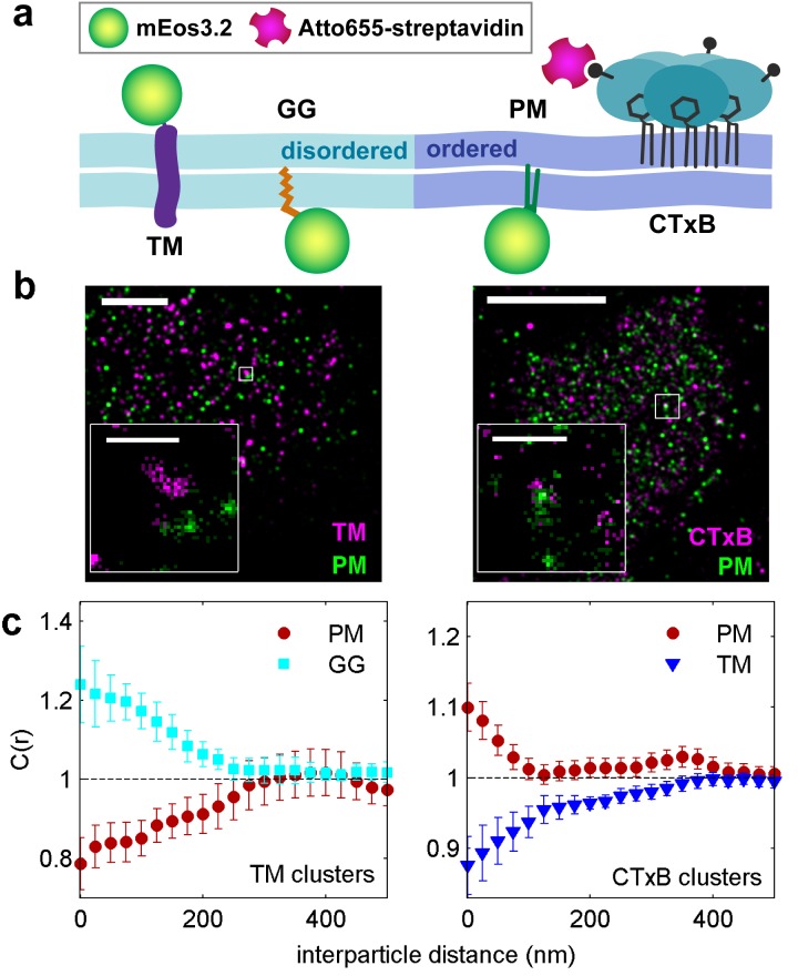
Figure 1.
Clusters of ordered or disordered phase markers create distinct membrane domains.
( a ) Schematic representation of minimal anchor peptides and their phase preference as determined from model membranes. Amino acid sequences and chemical structures are shown in Figure 1u2014figure s...
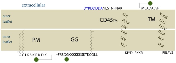
Figure 1u2014figure supplement 1.
Amino acidu00a0sequences of membrane anchors used in this study.
The amino acid sequence and post-translational modification of the four transiently expressed membrane anchors are shown. PM contains the 10 N-terminal amino acids from Lyn, which code for a myristoyl...
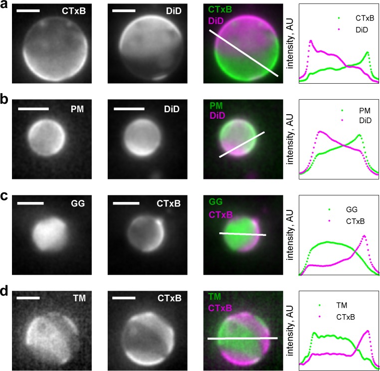
Figure 1u2014figure supplement 2.
Membrane anchors partition into different phases in GPMVs.
( a ) Alexa-555 CTxB and DiD-C 16 partition into different phases in GPMVs. CTxB is a well-established marker of the liquid-ordered phase, indicating that DiD-C 16 partitions into the liquid-disordere...
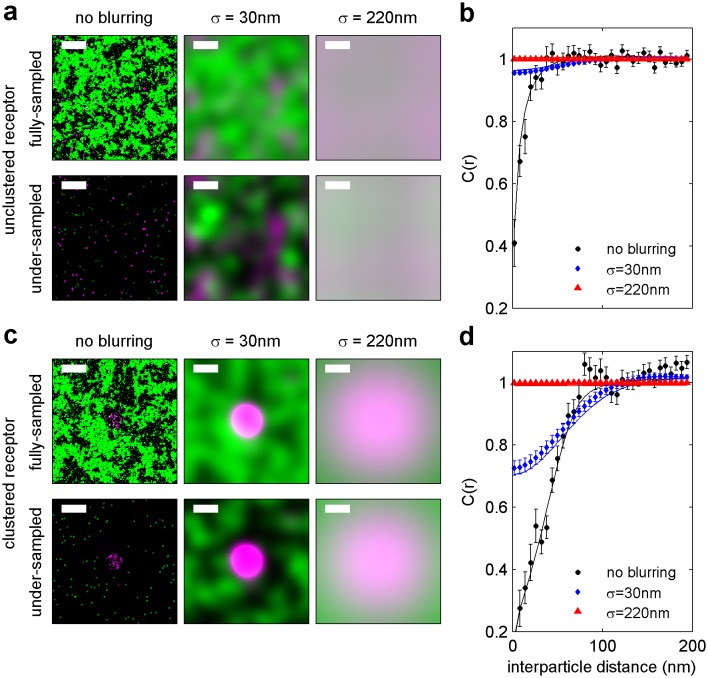
Figure 1u2014figure supplement 3.
Finite lateral resolution and incomplete spatial sampling impacts measured cross-correlations.
An Ising model simulated at Tu00a0=u00a01.05 times the critical temperature is used to demonstrate how finite lateral resolution and incomplete spatial sampling impacts measurements of cross-correlati...
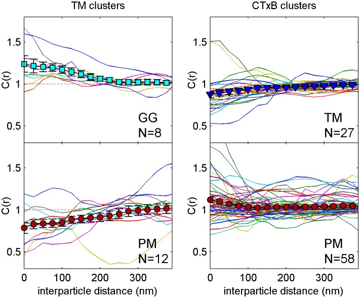
Figure 1u2014figure supplement 4.
Correlation functions from individual cells and average curves.
Colored lines are cross-correlation curves from individual cells that contribute to the average curves presented in Figure 1c . The large filled symbols represent the average curve and error bars indi...
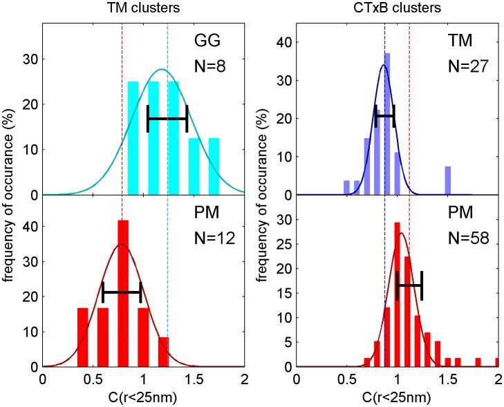
Figure 1u2014figure supplement 5.
Distribution of correlation function values closely matches the width expected from single measurement errors.
The histograms show the distributions of C(ru00a0<u00a025 nm) values obtained from single cell measurements under each of the conditions indicated. The curved lines indicate the best fit Gaussian f...
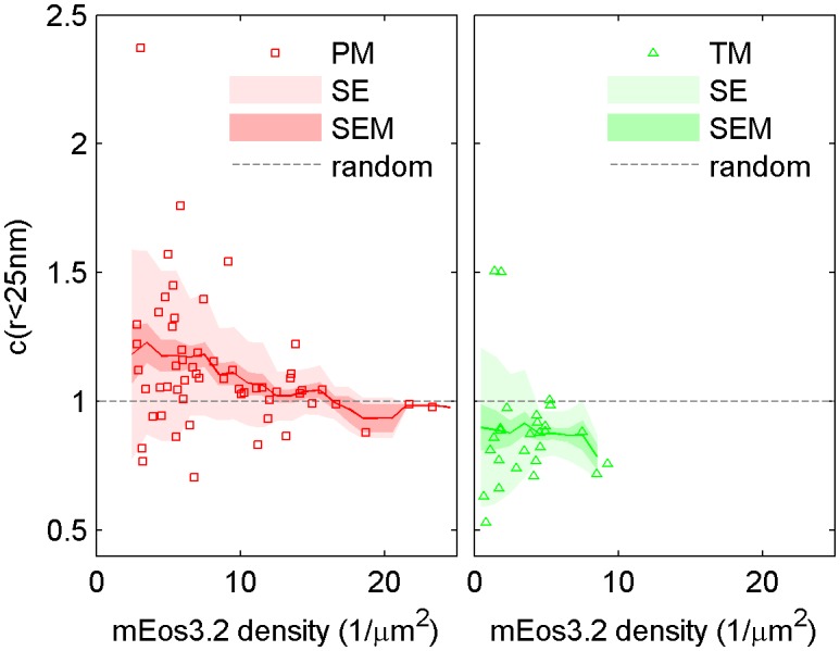
Figure 1u2014figure supplement 6.
The cross-correlationu00a0amplitude is weakly dependent on lipid probe expression level.
The first spatial bin of the cross-correlation C(ru00a0<u00a025 nm) is plotted against the density of the mEos3.2 probe for individual cells. Surface density of mEos3.2 is determined by fitting the...
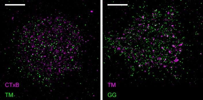
Figure 1u2014figure supplement 7.
Representative images from Figure 1 .
Representative images from conditions included in average curves but not shown in Figure 1 . Scale bars are 5 u00b5m. (left) Cells expressing mEos3.2-TM were labeled with CTxB-biotin that was then clu...
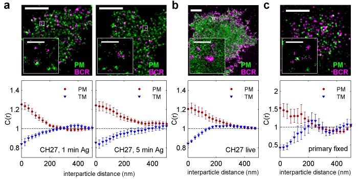
Figure 2.
BCR clusters localize within ordered membrane domains.
(Upper panels) Representative reconstructed super-resolution images of the BCR and PM in chemically fixed ( a ) and live ( b ) CH27 B cells, and chemically fixed primary B cells ( c ). Scale-bars are ...
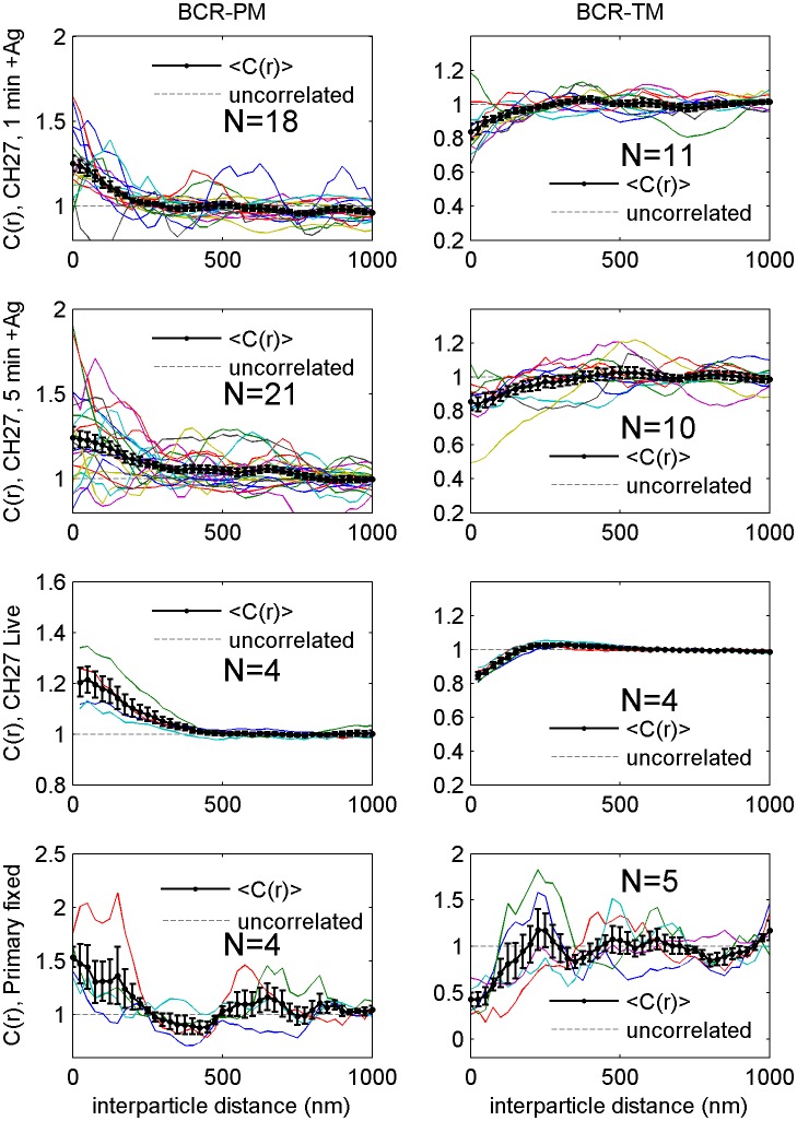
Figure 2u2014figure supplement 1.
Correlation functions from individual cells and average curves.
Cross-correlation curves from individual cells (colored lines) are averaged to obtain the curves shown in Figure 2 (black lines with errorbars). Error bounds indicate the standard error of the mean be...
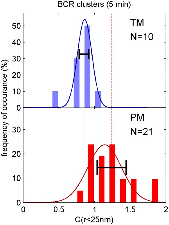
Figure 2u2014figure supplement 2.
Distribution of correlation function values closely matches the width expected from single measurement errors.
The histograms show the distributions of C(ru00a0<u00a025 nm) values obtained from single cell measurements in fixed cells where clustered BCR was imaged with the anchor probes indicated. The curve...
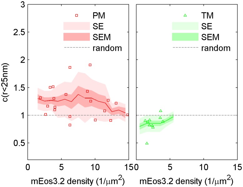
Figure 2u2014figure supplement 3.
Dependence of cross-correlation amplitudes on lipid probe expression levels.
The first spatial bin of the cross-correlation C(ru00a0<u00a025 nm) is plotted against the density of the mEos3.2 probe for individual cells. Surface density of mEos3.2 is determined by fitting the...
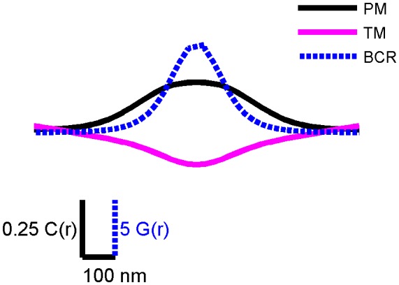
Figure 2u2014figure supplement 4.
PM and TM cross-correlation functions have a larger correlation length than BCR autocorrelation functions.
Conceptual diagram showing correlation functions from CH27 cells fixed 5 min following BCR clustering that were smoothed and made symmetric about the y axis. This figure highlights the length scale di...
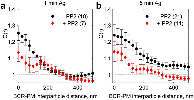
Figure 2u2014figure supplement 5.
Cross-correlations between clustered BCR and PM are reduced in the presence of a signaling inhibitor.
C(r) between PM and BCR in untreated cells and cells treated with 40 u00b5M of the Src kinase inhibitor PP2 and chemically fixed either one minute ( a ) or five minutes ( b ) following antigen additio...
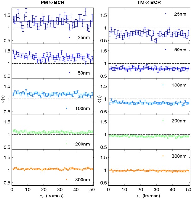
Figure 2u2014figure supplement 6.
Cross-correlations in live cells are calculated by averaging correlations between non-simultaneous frames.
Cross-correlations between probes in live cells suffer from poor statistics when only simultaneous frames are used to determine the cross-correlation. However cross-correlations between non-simultaneo...
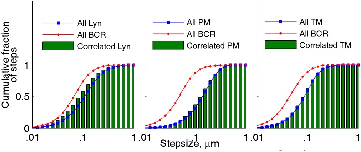
Figure 2u2014figure supplement 7.
The mobility of lipid probes is not altered when in close proximity to BCR clusters.
The mobility of anchors in close proximity to BCR clusters was probed in the same two-color live cell super-resolution experiments presented in Figure 2 . The cumulative step-size distributions shown ...
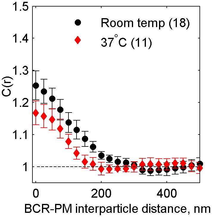
Figure 2u2014figure supplement 8.
Cross-correlations between clustered BCR and PM are reduced but still observable at physiological temperatures.
Average cross-correlation (C(r)) between PM and BCR at room temperature or at growth temperature (37u00b0C) one minute following antigen addition (N RT =u00a018, N 37 =u00a011). PM enrichment in BCR c...
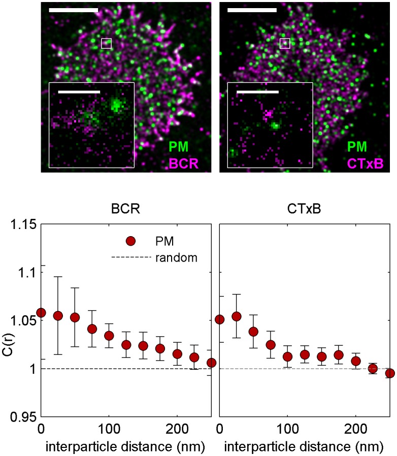
Figure 2u2014figure supplement 9.
Cross-correlations between PM and unclustered BCR or CTxB are near detection limits.
Representative images (top) showing cells expressing PM-mEos3.2 and labeled with Atto655 anti-IgM f(Ab) 1 (left) or Atto655-CTxB (right), where BCR or CTxB labels are not clustered with streptavidin. ...
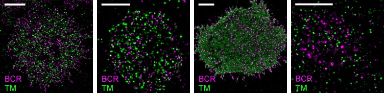
Figure 2u2014figure supplement 10.
Representative images from Figure 2 .
Representative images from conditions included in average curves but for which images are not shown in Figure 2 . Scale bars are 5 u00b5m. In all images, IgM BCR is labeled with f(Ab) 1 conjugated to ...
Video 1.
Reconstructed image timeu00a0lapse of single molecule localizations from live cell measurements of BCR (magenta) and PM (green).
Individual images are reconstructed using 100 frames (2u00a0s) of single molecule images, receptors are crosslinked at timeu00a0=u00a00, and the scale-bar is 5 u00b5m. Single BCR or PM proteins are im...
Video 2.
Reconstructed image timeu00a0lapse of single molecule localizations from live cell measurements of BCR (magenta) and TM (green).
Individual images are reconstructed using 100 frames (2u00a0s) of single molecule images, receptors are crosslinked at timeu00a0=u00a00, and the scale-bar is 5 u00b5m. Single BCR or TM proteins are im...
Video 3.
Reconstructed image timeu00a0lapse of single molecule localizations from live cell measurements of BCR (magenta) and Lyn kinase (green).
Individual images are reconstructed using 100 frames (2u00a0s) of single molecule images, receptors are crosslinked at timeu00a0=u00a00, and the scale-bar is 5 u00b5m. Single BCR or Lyn proteins are i...
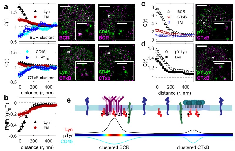
Figure 3.
Ordered domains promote tyrosine phosphorylation.
( a ) Average cross-correlation functions (C(r), left) and representative super-resolution images (right) demonstrating that full-length proteins and their minimal membrane anchors sort with respect t...
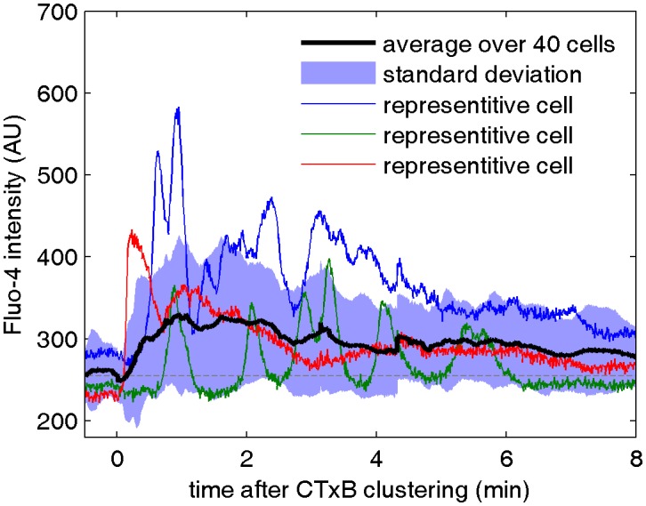
Figure 3u2014figure supplement 1.
Cell surface clustering of cholera toxin subunit B elicits calcium mobilization in B cells.
Cytosolic calcium levels were monitored in CH27 B cells both before and after biotinylated CTxB was clustered with streptavidin using the calcium indicator Fluo-4 as described in Methods. Colored curv...
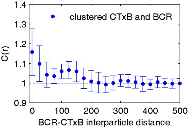
Figure 3u2014figure supplement 2.
CTxB clusters are not highly correlated with BCR.
Average cross-correlation between clustered CTxB and BCR indicates that these two proteins are not colocalized. Biotinylated CTxB was clustered by streptavidin conjugated to Atto 655 and cells were fi...
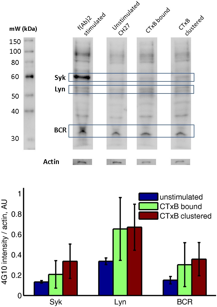
Figure 3u2014figure supplement 3.
Subtle increases in protein phosphotyrosine levels in response to CTxB clustering are suggested by western blots of whole cell lysates.
CH27 cells were treated as indicated above lanes, and anti-phosphotyrosine western blots were performed using cell lysates. The top shows a representative western blot, where identity of Syk, Lyn, and...
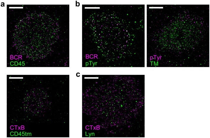
Figure 3u2014figure supplement 4.
Representative images from Figure 3 .
Representative images from conditions included in average curves in Figure 3 are shown here. Scale bars are 5 u00b5m. ( a ) Cells stained for CD45 (top) or expressing CD45tm (bottom) where either BCR ...
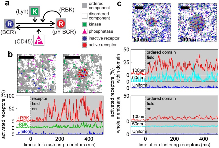
Figure 4.
A model linking receptor clustering to receptor phosphorylation.
( a ) Schematic representation of the model described in the main text. Possible biological analogs of model components are indicated, with u201cRBKu201d representing receptor-bound kinases. ( b ) Sim...
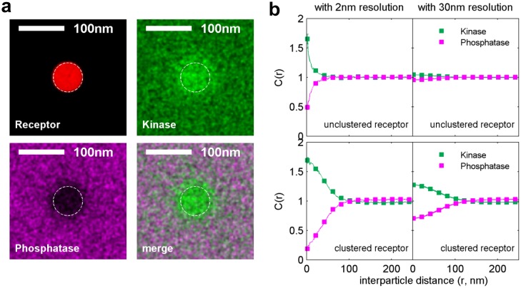
Figure 4u2014figure supplement 1.
Simulations naturally reproduce experimental kinase and phosphatase distributions with respect to the BCR.
( a ) Time-averaged positions of the receptor, kinase, and phosphatase in simulations. Kinases are recruited and phosphatases are excluded from clustered BCR. The location of the receptor cluster is i...
Video 4.
Simulated timeu00a0course of receptor activation upon clustering in a heterogeneous membrane.
Simulations are conducted as described in Methods. The positions of receptors (circles), kinases (green squares), and phosphatases (magenta triangles) are shown at 1 ms intervals (representing 1000 si...
Video 5.
Simulated timeu00a0course of receptor activation upon clustering in a heterogeneous membrane without the positive feedback loop accomplished through receptor bound kinases.
Simulations are conducted as described in Methods. The positions of receptors (circles), kinases (green squares), and phosphatases (magenta triangles) are shown at 1 ms intervals (representing 1000 si...
Video 6.
Simulated timeu00a0course of receptor activation upon clustering in a uniform membrane.
Simulations are conducted as described in Methods.u00a0The positions of receptors (circles), kinases (green squares), and phosphatases (magenta triangles) are shown at 1 ms intervals (representing 100...
Video 7.
Simulated timeu00a0course of receptor activation upon stabilization of a large ordered domain.
Simulations are conducted as described in Methods. The positions of receptors (circles), kinases (green squares), and phosphatases (magenta triangles) are shown at 1 ms intervals (representing 1000 si...
Video 8.
Simulated timeu00a0course of receptor activation upon stabilization of a small, ordered domain.
Simulations are conducted as described in Methods. The positions of receptors (circles), kinases (green squares), and phosphatases (magenta triangles) are shown at 1 ms intervals (representing 1000 si...
Video 9.
Simulated timeu00a0course receptor activation state within a uniform membrane with an applied field.
Simulations are exactly as described for Video 7 but unspecified membrane components are all of the same type (ordered in this case). The positions of receptors (circles), kinases (green squares), and...
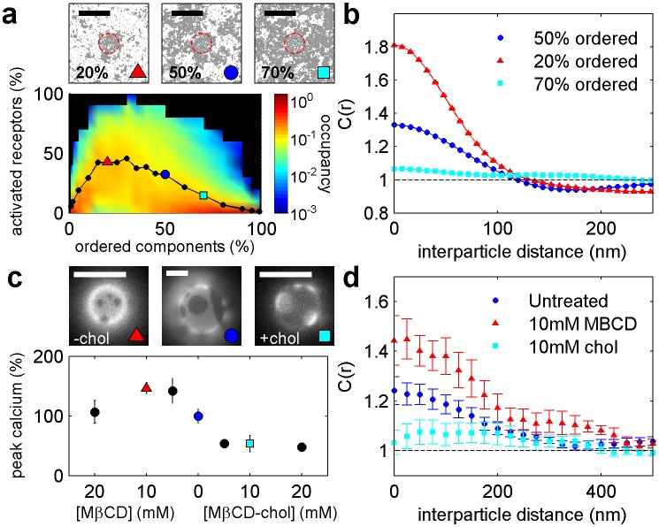
Figure 5.
Phosphorylation model predicts the response to changing the fraction of ordered and disordered components.
( a ) Representative snap-shots (top) and histograms showing receptor phosphorylation (bottom) in simulations run with different fractions of ordered and disordered components (grey and white pixels r...
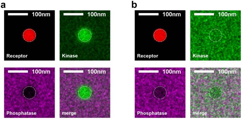
Figure 5u2014figure supplement 1.
Kinase and phosphatase partitioning into receptor clusters change dramatically as the surface fraction of ordered components is varied.
Time-averaged positions of the receptor, kinase, and phosphatase in simulations with ordered components making up 20% ( a ) or 80% ( b ) of the simulated membrane. The location of the receptor cluster...
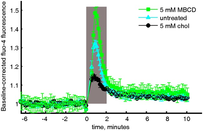
Figure 5u2014figure supplement 2.
Averaged and baseline-corrected Fluo-4 intensity curves.
Relative Fluo-4 intensity of CH27 cells stimulated with anti-IgM f(Ab) 2 with either Mu03b2CD treatment, cholesterol treatment, or no treatment. The curves were integrated within the gray box to give ...
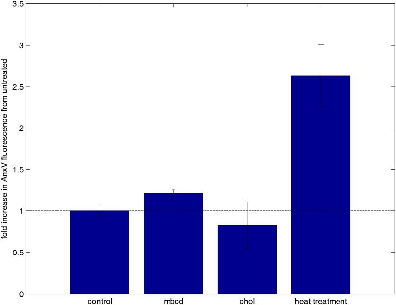
Figure 5u2014figure supplement 3.
Cholesterol treatments do not alter annexin Vu00a0staining.
CH27 cells were treated with either 10 mM Mu03b2CD, 10 mM Mu03b2CD loaded with cholesterol, or control buffer in an identical manner as cells from Figure 3c where calcium release was tested. A positiv...
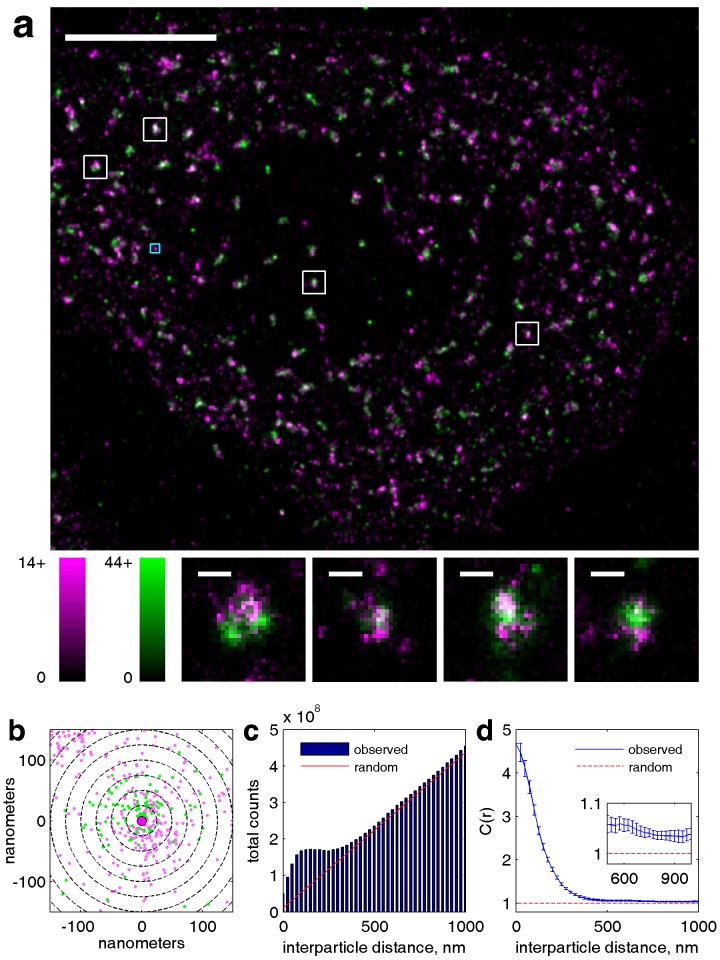
Figure 6.
Our cross-correlation methodology applied to doubly labeled clathrin.
( a ) Two-color super-resolution image of a HeLa cell expressing two distinct labeled clathrin heavy chain constructs is shown. Clathrin heavy chains associate strongly in clathrin coated pits, and th...
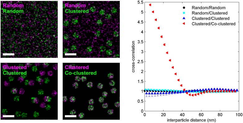
Figure 6u2014figure supplement 1.
The cross-correlation function detects deviations in the co-distribution of localizations from random.
Four simulations of two-color localization distributions are shown, where the spatial distribution of the localization is given by the labels in the top left of the images. For clustered distributions...
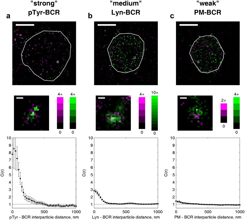
Figure 6u2014figure supplement 2.
The amplitude of the cross-correlation reflects differences in enrichment magnitude and interaction strength.
Example cells from three different experiments are shown to illustrate the range of values the cross-correlation function can take for various types of interactions. ( a ) An example of a strong enric...
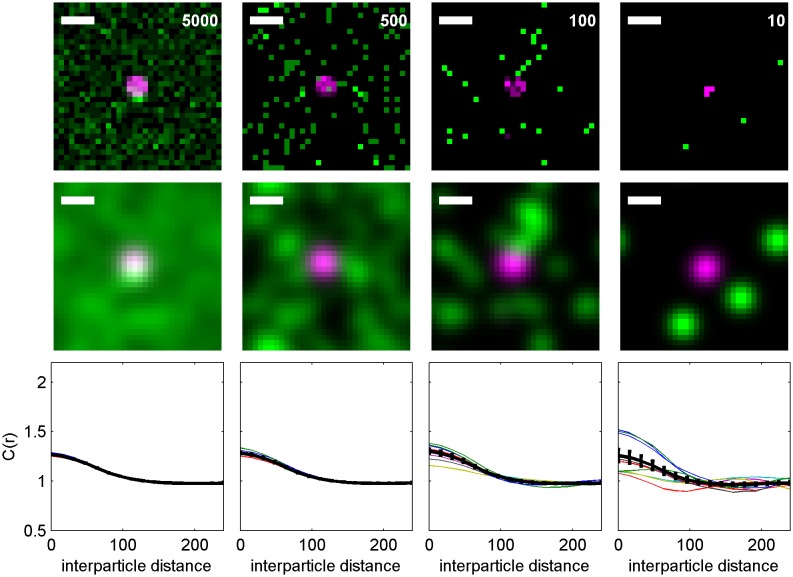
Figure 6u2014figure supplement 3.
Cross-correlations detect co-clustering even when there is a low surface density of labeled molecules.
An Ising model containing kinase (green) and clustered receptors (magenta) is used to demonstrate how the surface density of labeled proteins impacts correlation functions. (top) Representative histog...
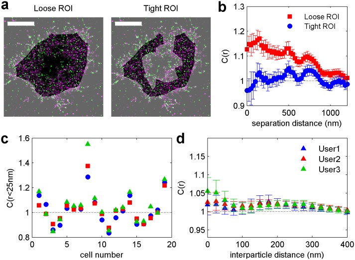
Figure 6u2014figure supplement 4.
Membrane topology gives rise to long-range structure in cross-correlations, but can be removed by careful selection of regions of interest (ROI).
( a ) Reconstructed super-resolution image of a CH27 B cell in which part of the cell has detached from the coverslip surface leading to a reduction in localizations in the center of the cell, which i...
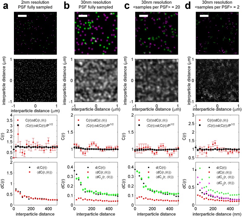
Figure 6u2014figure supplement 5.
Estimation of the variance associated with a cross-correlation measured on a single super-resolution fluorescence localization image.
Simulations containing randomly distributed green and magenta points are used to identify the sources of error typically found in cross-correlations tabulated from images acquired using super-resoluti...
Figure images are served from the NIH/NLM PubMed Central Open Access Subset or Europe PMC; copyright remains with the publishers and authors.
💬 Discussion
0 commentsNo comments yet. Be the first to start a discussion!
Leave a Comment