Abstract
Abstract Multiplexed mRNA profiling in the spatial context provides new information enabling basic research and clinical applications. Unfortunately, existing spatial transcriptomics methods are limited due to either low multiplexing or complexity. Here, we introduce a spatialomics technology, termed Multi Omic Single-scan Assay with Integrated Combinatorial Analysis (MOSAICA), that integrates in situ labeling of mRNA and protein markers in cells or tissues with combinatorial fluorescence spectral and lifetime encoded probes, spectral and time-resolved fluorescence imaging, and machine learning-based decoding. We demonstrate MOSAICA’s multiplexing scalability in detecting 10-plex targets in fixed colorectal cancer cells using combinatorial labeling of five fluorophores with facile error-detection and removal of autofluorescence. MOSAICA’s analysis is strongly correlated with sequencing data (Pearson’s r = 0.96) and was further benchmarked using RNAscope TM and LGC Stellaris TM . We further apply MOSAICA for multiplexed analysis of clinical melanoma Formalin-Fixed Paraffin-Embedded (FFPE) tissues. We finally demonstrate simultaneous co-detection of protein and mRNA in cancer cells.
🔬 Techniques
🔭 Microscopes
✨ Fluorophores
🧪 Sample Preparation
🔬 Cell Lines
🏭 Microscope Brands
🧪 Reagent Suppliers
🔴 Lasers
📷 Detectors
💻 Software Details
💾 Data Repositories
🏛️ Research Organizations (ROR)
Affiliated research institutions:
📋 Methods
Ethical statement
We confirm this research complies with all relevant ethical regulations. The University of California, Irvine Institutional Review Board (IRB) approved this study for IRB exemption under protocol number HS# 2019–5054. All human melanoma FFPE cases were de-identified samples to the research team at all points and therefore considered exempt for participation consent by the IRB.
Primary probe design
A set of primary probes were designed for the transcript of each gene. A python code was used to rapidly design the primary probes while controlling various aspects of the probes such as GC content, length, spacing, melting temp, and prohibited sequences. To begin, probes are designed using exons within the coding sequence region. However, if that region does not provide over 40 probes, the exons from the coding and untranslated regions are used. The candidate probes are then aligned to the genome using Bowtie2, an NGS aligner, to determine if these probes are specific. Probes that are determined specific are then aligned to the RNA sequencing data on the UCSC Genome Browser, further eliminating probes that do not align to regions with an adequate number of reads. While mapping the probes to the genome on the UCSC Genome Browser, the probes are aligned with BLAT (BLAST-like alignment tool). A local BLAST query was run on the probes for the expressed genes in the panel to eliminate off-target hits. For this experiment, each expressed gene had the maximum number of probes that could be designed with our pipeline and requirements. The final primary probe design included two assigned readout sequences of the secondary probe with a “TTT” connector in between, another connector, then one of the probes specific for the transcript of that gene. The primary probes were ordered from Sigma Aldrich and pooled together for the transcript of each gene. The sequences of all probes used in this study are listed in Supplementary Data 1 .
Show full methods section
Ethical statement
We confirm this research complies with all relevant ethical regulations. The University of California, Irvine Institutional Review Board (IRB) approved this study for IRB exemption under protocol number HS# 2019–5054. All human melanoma FFPE cases were de-identified samples to the research team at all points and therefore considered exempt for participation consent by the IRB.
Primary probe design
A set of primary probes were designed for the transcript of each gene. A python code was used to rapidly design the primary probes while controlling various aspects of the probes such as GC content, length, spacing, melting temp, and prohibited sequences. To begin, probes are designed using exons within the coding sequence region. However, if that region does not provide over 40 probes, the exons from the coding and untranslated regions are used. The candidate probes are then aligned to the genome using Bowtie2, an NGS aligner, to determine if these probes are specific. Probes that are determined specific are then aligned to the RNA sequencing data on the UCSC Genome Browser, further eliminating probes that do not align to regions with an adequate number of reads. While mapping the probes to the genome on the UCSC Genome Browser, the probes are aligned with BLAT (BLAST-like alignment tool). A local BLAST query was run on the probes for the expressed genes in the panel to eliminate off-target hits. For this experiment, each expressed gene had the maximum number of probes that could be designed with our pipeline and requirements. The final primary probe design included two assigned readout sequences of the secondary probe with a “TTT” connector in between, another connector, then one of the probes specific for the transcript of that gene. The primary probes were ordered from Sigma Aldrich and pooled together for the transcript of each gene. The sequences of all probes used in this study are listed in Supplementary Data 1 .
Secondary probe design
Secondary probe structures were based on the design from the Zhuang group 56 . In short, the 20-nt, three-letter readout sequences were designed by generating a random set of sequences with the per-base probability of 25% for A, 25% for T, and 50% for G. Sequences generated in this fashion can vary in their nucleotide content. To eliminate outlier sequences, only sequences with a GC content between 40% and 50% were kept. In addition, sequences with internal stretches of G longer than 3 nucleotides were removed to eliminate the presence of G-quadruplets, which can form secondary structures that inhibit synthesis and binding. To remove the possibility of significant cross-binding between these readout sequences, algorithms from previous reports were used to identify a subset of these sequences with no cross-homology regions longer than 11 contiguous bases 56 . Probes were then checked with BLAST to identify and eliminate sequences with contiguous homology regions longer than 11 nucleotides to the human transcriptome. From the readout sequences satisfying the above requirements, 16 were selected.
Cell culture Human embryonic kidney
(HEK293T) cells (632180; Takara) were cultured in DMEM (10-013-CV; Corning) supplemented with 10% FBS (1500-500; Seradigm) and 1% penicillin (25–512; GenClone).
Human colorectal adenocarcinoma
(SW480) cells were cultured in DMEM with high glucose (SH30081.02; HyClone) supplemented with 10% FBS (1500-500; Seradigm), 1x L-Glutamine (25–509; GenClone), and 1% penicillin (25–512; GenClone). SW480 cells were FACS-sorted based on surface marker ROBO-1, and ROBO + and ROBO- cells were used in Fig. 4 and Fig. 6 , respectively. The cells were plated into 8-well chambers and then fixed. The eight-well plates (155409; Thermo Scientific) for HEK293-T and SW480 cells were coated with fibronectin bovine plasma (F1141-2MG; Sigma Aldrich) before seeding cells onto the 8-well plates. All cultures were grown at 37 °C with 5% CO 2 . mNeonGreen cell engineering A mNeonGreen construct was transfected into HEK293T-X cells with FuGENE HD Transfection Reagent (E2311; Promega). The cells were then selected with puromycin (NC9138068; Invivogen) and Zeocin (AAJ67140XF; Alfa Aesar) 3 days after transfection.
Preparation of fixed cells in cell chambers
When the cells reached 70% confluency, cells were fixed for 30 min using 4% paraformaldehyde (15710; Electron Microscopy Science), then washed with PBS 3 times. The cells were then incubated with sodium borohydride (102894; MP Biomedicals) for 5 min and washed with PBS 3 times. 0.5% Triton X-100 (T8787-100ML; Sigma-Aldrich) in PBS was incubated in each well for 5 min and cells were washed with 2x SSCT (2x SSC with 0.1% TWEEN® 20 (P9416-100ML; Sigma-Aldrich). For storage, cells were left in 70% ethanol at 4 °C. Preparation of FFPE tissues The University of California, Irvine Institutional Review Board (IRB) approved this study for IRB exemption under protocol number HS# 2019–5054. All human melanoma cases were de-identified samples to the research team at all points and therefore considered exempt for participation consent by the IRB. Fully characterized human patient skin melanoma FFPE tissues with an immune cell score of brisk were obtained from the UCI dermatopathology center then sectioned to 5 µm slices using a rotary microtome, collected in a water bath at 35 °C, and mounted to positively charged Fisher super frost coated slides. The tissue sections were then baked at 60 °C for 1 h. For antigen unmasking, slides were deparaffinized, rehydrated then followed by target retrieval (with citrate buffer).
Primary probe hybridization
Blocking buffer containing 100 mg/ml Dextran sulfate sodium salt (D8906-100G; Sigma-Aldrich), 1 mg/ml Deoxyribonucleic acid from herring sperm (D3159-100G; Sigma-Aldrich), 0.01% Sodium Azide (S2002-100G; Sigma-Aldrich), 0.01% tween, and 15% ethylene carbonate (AC118410010; Fisher Scientific) in 2x sodium saline citrate (SSC) was added to the fixed cells or tissues and incubated at 60 °C for 8 min and then at 37 °C for 7 min. Following this preblock step, primary probes with 5 nM of each probe in blocking buffer were added to the samples and incubated at 60 °C for 30 min and then overnight at 37 °C.
Secondary probe hybridization
Once the primary probe solution is removed, the sample is washed with 2x Saline-Sodium Citrate Tween (SSCT) twice. Wash buffer (2xSSCT with 10% ethylene carbonate) is used for 3 washes and incubated in 60 °C for 5 min each time. Blocking buffer is added and incubated at room temperature for 5 min. The sample is then incubated in a solution with 5 nM of the secondary probes in blocking buffer at 37 °C for an hour. The sample is washed with 2x SSCT twice before using wash buffer to wash 3 times and incubated in 42 °C for 5 min each time. For the first wash, 10 mg/mL Hoechst (H3570; Invitrogen) is diluted 1:1000 in PBS and added to cells. Later, the wash buffer is then removed and replaced with glycerol mounting media and ready for imaging. Codetection of protein and mRNA Prior to mRNA labeling, fixed SW480 cells were blocked with 1% Bovine Serum Albumin (RLBSA50; VWR), 0.1% TWEEN® 20, 1:1,000 Sodium Azide, 0.2 U/ml Protector RNase inhibitor (3335399001; Sigma-Aldrich), and 1 mM DTT in RNAse-free PBS (AM9625; Life Technologies) for 30 min at room temperature. These cells were then washed 3 times with 0.1% TWEEN® 20 in RNAse-free PBS for 5 min each wash at room temperature. Antibody solutions containing 1:1,000 Mouse anti-Tubulin (3873BF; Cell Signaling) and 1:200 Rabbit anti-Vimentin (5741BF; Cell Signaling) in the same blocking buffer were subsequently added to the samples and incubated overnight at 4 °C. Following 3 additional washes with 0.1% TWEEN® 20 in RNAse-free PBS for 5 min each at room temperature, antibody solutions containing fluorescently labeled 1:200 Donkey anti-Mouse Alexa-488 ( R37114 ; Fisher Scientific) and 1:200 Donkey anti-Rabbit TRITC (711-025-152; Jackson Laboratories) in the same blocking buffer were added at room temperature for 1 h. After 3 washes with RNAse-free PBS with 0.1% TWEEN® 20 for 10 min each wash at room temperature, 4% PFA in PBS was added for 15 min at room temperature. These cells were then washed 3 times with 0.1% TWEEN® 20 in PBS at room temperature for 5 min. For mRNA labeling, the previously described methods regarding primary and secondary probe hybridization were utilized. LGC Stellaris TM LGC Stellaris TM RNA FISH probes (Biosearch Technologies, CA, USA) were used, with 48 × 20 mer fluorophore-conjugated oligos tiling the length of the target transcript. The POLR2A probe set were supplied as predesigned controls conjugated to Quasar 570 fluorophores. Labeling/staining was carried out as described in the LGC Stellaris TM protocol for adherent mammalian cells. The POLR2A probe sets were used at 50 nM. RNAscope TM The FFPE tissue sections were deparaffinized before endogenous peroxidase activity was quenched with hydrogen peroxide. Target retrieval was then performed, followed by protease plus treatment. The fixed cells pretreatment included treatment with hydrogen peroxide and protease 3. The RNAscope TM assay was then performed using the RNAscope TM Multiplex Fluorescent V2 kit and Akoya Cy5 TSA fluorophore. The positive control ( POLR2A ) and negative control ( dapB ) were in C1.
Microscopy Imaging
Our samples can be imaged with any instrument provided that it has spectral and lifetime acquisition capabilities. Our measurements were taken on three separate instruments, a wide-field and two confocal microscopes. A generic spectral-FLIM scanning confocal instrument setup is depicted in Supplementary Fig. 9 . For validation of fluorophores and their spectral and lifetime signatures, measurements were taken on a 2-channel ISS Alba5 STED platform. This system is equipped with a pulsed white laser (NKT SuperK EXTREME) system where the excitation wavelength(s) can be selected with an acousto-optic tunable filter (NKT SuperK SELECT). Single photons were detected with avalanche photodiode detectors (Excelitas Technologies) and their arrival times with respect to the stimulating frequency (78 MHz) were measured with a FPGA-based electronic board (ISS FastFLIM). Imaging was achieved by fast beam scanning with galvo mirrors and 3D stacks of images were acquired with a z-piezo mount on the objective. For measurements of multiplexed/combinatorial labeling and detection experiments (Fig. 4 and Fig. 5 ), we utilized a Leica SP8 with the Falcon module. This platform employs a white light laser and an acoustic optic beam splitter dichroic, and the Leica hybrid detectors with excitation band selectable by means of a prism. 3D measurements of cells and tissue samples were taken with a 100x plan apochromat oil objective with a numerical aperture of 1.40, yielding images with an x-y resolution of 100 nm and z-spacing of 500 nm. For epifluorescence measurements (Supplementary Fig. 2 and Supplementary Fig. 3 ), images of labeled mRNA transcripts were taken on an inverted Ti-E using a 100× plan apochromat oil objective with a numerical aperture of 1.40. Samples were illuminated with a Spectra-X (Lumencor) LED light source at the 395 nm, 470 nm, 555 nm and/or 640 nm excitation wavelengths. Images were acquired with an Andor Zyla 4.2 sCMOS camera at 4 K resolution with 6.5 µm pixels.
Image Processing
A custom set of scripts were written in MATLAB to process the acquired image stacks, identify individual transcripts and assign each of them to each gene expression target. After reconstructing the images out of the digital list of photons, the analysis runs in parallel a 3D blob detection pipeline on the intensity image stacks to identify each transcript and on the other a clustering pipeline on the phasor-transformed lifetime/spectral phasor data to detect distinct spectral/lifetime populations. A classifier then assigns pixels as belonging to a particular expressed gene. The whole pipeline is depicted in Supplementary Fig. 10 . Briefly, the intensity 3D stacks are run through a blob detection algorithm that was developed in order to identify each transcript. The images can be seen as a 3D space where the transcripts appear as spherically symmetric locations with a radial increase in intensity, namely puncta. The algorithm first computes the low-frequency background noise by means of a median filter with a kernel 10 times the size of the expected puncta (the diffraction limit of the instrument, in our case around 250 nm). This low-frequency background is subtracted from the high-pass filtered data obtained by convolving by a gaussian filter of the expected size of the puncta. This on one hand enhances the puncta in the image by giving a prominence value at each pixel with respect to the surrounding regions and on the other suppresses noise in the images. A search for local maxima is performed by finding the locations where the gradient goes to zero and the divergence of the gradient is negative. Once the centers in the 3D coordinate space are obtained the size, absolute brightness and prominence of each puncta is measured. In parallel, the raw photon counts are used to construct the photon arrival time histogram and photon spectral histogram at each pixel. Phasor transforms are applied to each pixel in each image of the 3D stack in order to construct the stacks’ phasor plot. This phasor data is in general a 4-dimensional, each pixel in the intensity image has four additional coordinates; two for the spectral phasor transform plus two for the lifetime phasor transform. The phasor coordinates are clustered using Gaussian Mixture Models 57 . We used an initial experiment tagging the transcripts of housekeeping genes in order to guarantee that all expected populations were present and we trained the Gaussian Mixture Model using this initial experiment. This pretrained model is then applied to the new sets of data in order to classify each pixel into one of the clusters allowing for the presence of empty clusters. The number of clusters N intuitively should be the number of distinct fluorescent probes or different combinations of probes used to tag the sample, but one must allow for additional populations in the sample, e.g., autofluorescent species. For this reason, in the training of the Gaussian Mixture Models we allowed for one additional cluster to account for autofluorescence and noise. Finally, by computing the mean phasor coordinates of the pixels within each detected puncta, we can compute the phasor position of each puncta and assign a gene expression label to it by a priori knowing the expected positions of each combination of probes depending on the spectra and lifetime of the probes. To obtain the number of counts per cell, DAPI image stacks are segmented by means of simple thresholding, estimating the threshold value by hard-splitting of the histogram of photon counts in the channel. The 3D segmented nuclei are then iteratively grown by convolution by a minimal 3x3x3 kernel. This convolution is applied at each pixel of the edge of the segmented volume until no available space is left between the segmented volumes. This yields a division of the imaged volume into polyhedra where each face is exactly the plane bisecting the two closest nuclei edges. This process is analogous to a Voronoi tessellation using the surface of the nuclei instead of points. In the cell culture experiments, to normalize by cell volume, we used a normalized mean cell volume of 3000 µm 3 since a cell marker was not utilized and the imaged volume thickness (5 µm) was less than the actual cell thickness. To obtain mean counts per cell, total detected puncta counts was divided into the total imaged cellular volume and then multiplied by an estimated mean cell volume of 3000 µm 3 . The total cellular volume was obtained by an intensity threshold segmentation of the background cellular autofluorescence over the gaps between cells.
Simulations
In order to test the detection and classification pipeline, we wrote a set of scripts to simulate spectral/lifetime data which provided a ground truth towards detection and accurate classification debugging. This data generation script allows randomly distributing N diffraction-limited transcripts in an arbitrarily big 3-dimensional space, each with a gaussian intensity profile. We simulated our transcript gaussian profile with a X-Y standard deviation of 200 nm and a Z standard deviation of 500 nm, a peak intensity of 1 ± 0.3 (the intensity becomes relevant when simulating background noise). In the simulation run that we used to test the crowding limitations of the system we simulated tagging the transcripts of genes with couples out of a total of 12 fluorescent probes; 4 distinct spectral probes and 3 distinct lifetimes in each, yielding a total of documentclass[12pt]{minimal} usepackage{amsmath} usepackage{wasysym} usepackage{amsfonts} usepackage{amssymb} usepackage{amsbsy} usepackage{mathrsfs} usepackage{upgreek} setlength{oddsidemargin}{-69pt} begin{document}$$left(begin{array}{c}12\ 2end{array}right)=66$$end{document} 12 2 = 66 possible expressed genes. We generated the simulated images in a cubic space of 10 × 10 × 10 µm, discretized as an image stack of 33 images of 1000 × 1000 pixels (yielding a voxel resolution of 100 × 100 × 300 nm). This volume was generated containing increasing densities of transcripts, ranging from a single transcript of each gene (66 transcripts) up to 2000 transcripts of each gene (132k transcripts) and for each possible value of density a total of 10 iterations each time. These 20k simulated image stack sets were individually processed by our image processing pipeline and the transcript position and labelling obtained by the pipeline was compared to the known ground truth of the generated data. This simulation provided a benchmark of the density limitations of the method but at the same time giving an idea of the underestimation of the number of transcripts as a function of local density. The simulations allowed us to model the estimated number of overlapping transcripts as a function of density. A similar set of simulations was run by emulating the conditions in the 10-plex experiment (Fig. 4 ) where the transcripts of genes are tagged with combinations of two out of five probes. The 20k iterations for different densities allowed to plot the density of the classification obtained after detection compared to the real number of transcripts in the simulations. This simulation was fit to the probabilistic model obtained from calculating the number of transcripts that are not overlapped in space (see next section), from which the true number of puncta was extracted (see Supplementary Fig. 4 ). Overlapping probability The fraction of puncta that do not overlap with any other puncta depends on the total number of puncta present in the volume of study and the relative proportion between said total volume and the volume of each individual puncta. The following expression is obtained as the product of N-1 times the fraction of available space having removed the volume occupied by one transcript: 2 documentclass[12pt]{minimal} usepackage{amsmath} usepackage{wasysym} usepackage{amsfonts} usepackage{amssymb} usepackage{amsbsy} usepackage{mathrsfs} usepackage{upgreek} setlength{oddsidemargin}{-69pt} begin{document}$$frac{n}{N}={left(1-frac{{v}_{i}}{{V}_{T}}right)}^{N-1}$$end{document} n N = 1 − v i V T N − 1 where n is the number of isolated puncta, N is the total number of puncta, v i is the volume of each puncta and V T is the total volume (simulated or scanned). The real number of transcripts N cannot be analytically isolated from the previous equation, but one can graphically obtain it. Due to the fact that the transcripts are sub-diffraction limit, the value of v i is simply the volume of the point spread function of the instrument. Using the detected number of counts in an experiment n= 13.5k and the estimated total imaged cellular volume of 68 kµm 3 , both obtained from two image stacks shown in Fig. 4 , we proceeded to estimate the real number of transcripts present in the sample using the previous expression. Assuming an interval of possible volumes for the transcripts (instrument PSF) between 0.1 and 0.3 µm 3 we obtained an estimated percentage of overlapping puncta in the interval [2.0, 6.6]%. This range of values is in agreement with the number of puncta that we detected in more than two channels in the 10-plex experiments (3.7%) and in the tissue experiments (2.1%). See Supplementary Fig. 4 for additional details such as expression (2) plotted as a function of the density of transcripts.
Sequencing Data Colorectal cancer SW480 cell bulk
RNA sequencing (unpublished data) was analyzed with DESeq2. Average expression is then obtained for comparison to the MOSAICA puncta count for each expressed gene. For the human skin melanoma FFPE tissue, the patient sample did not have corresponding sequencing data. RNA sequencing data were obtained from publicly available data from The Cancer Genome Atlas (TCGA), available on the National Cancer Institute (NCI) Genomic Data Commons (GDC) data portal, from 5 human skin melanoma FFPE biopsy thigh punch samples [Entity ID: TCGA-EE-A2GO-06A-11R-A18S-07, TCGA-EE-A20C-06A-11R-A18S-07, TCGA-YG-AA3N-01A-11R-A38C-07, TCGA-DA-A95Z-06A-11R-A37K-07, TCGA-GN-A26C-01A-11R-A18T-07]. The sequencing data were analyzed with HTseq and normalized for sequencing depth and gene length using Fragments Per Kilobase Million. The average of the 5 patient samples for each transcript were used for correlation graphs with MOSAICA puncta count. Experimental replicates and reproducibility Figure 3 is a conceptual figure and a single experiment was used as an example without replicates. For the 10-plex cell culture experiments (Fig. 4 ), we ran 3 experimental replicates from which we imaged 6 fields of view (100 × 100 × 5 µm each), with 364 cells in total. In these image stacks, a total of 65,562 puncta were detected where 38,056 were assigned and 27,506 were unassigned to a target. The unassigned counts were further categorized based on assumed overlapping errors (2439) or as undetermined counts (25,053). In the associated negative controls, a total of three experiments were performed, of which we imaged 4 fields of view containing 189 cells total. In these experiments, a total of 2034 puncta were detected, of which 61 were classified as targeted expressed genes due to the expected spectral and lifetime signature and 1959 were classified as undetermined. The tissue experiments with a 6-plex gene expression panel were replicated a total of 2 times yielding 2 fields of view of 130 × 130 × 3 µm each, together containing 174 cells (Fig. 5 ). A total of 2934 puncta were detected of which 1770 were assigned to a target and 1164 were unassigned, the latter group divided into 62 puncta unassigned due to overlap and 1100 labelled as undetermined. In the associated negative controls, we ran a total of 3 experiments yielding 3 fields of view and 375 cells. In these fields of view, 390 puncta were detected, of which 43 were assigned to the transcripts of targeted genes. Of the other 347, only 4 were assigned to overlap and 339 to undetermined. The protein-mRNA codetection experiment in Fig. 6 is a pilot experiment for demonstration purpose and there is no replicate for it. Additional 8-plex and 2-plex experiments were performed on cell cultures, two replicates each, yielding a total of 143 and 130 profiled cells, respectively. Quantification of the experimental replicates by means of cross correlation is presented in Supplementary Fig. 5 and Supplementary Fig. 6 .
Statistical Analysis
When comparing distributions of puncta counts, signal-to-noise ratios, and intensity values, Student (two-sided) t-tests were performed against the probability that the measured distributions belong to distributions with equal means. The reported probability values in the figures are symbolized with (* for p < 0.05, ** for p < 0.01, *** for p < 10 −3 , and **** for p < 10 −4 ). Pearson correlation coefficient was computed to determine the correlation between the average expression level to the puncta count of each transcript and to compare within replicates of same experiments. For comparison of 2-plex gene expression counts, we implemented a binomial test where we used the obtained proportion of counts from the 10-plex experiments as the reference probability (Supplementary Fig. 6 ). Reporting summary Further information on research design is available in the Nature Research Reporting Summary linked to this article.
Experimental replicates and reproducibility Figure 3 is a conceptual figure and a single experiment was used as an example without replicates. For the 10-plex cell culture experiments (Fig. 4 ), we ran 3 experimental replicates from which we imaged 6 fields of view (100 × 100 × 5 µm each), with 364 cells in total. In these image stacks, a total of 65,562 puncta were detected where 38,056 were assigned and 27,506 were unassigned to a target. The unassigned counts were further categorized based on assumed overlapping errors (2439) or as undetermined counts (25,053). In the associated negative controls, a total of three experiments were performed, of which we imaged 4 fields of view containing 189 cells total. In these experiments, a total of 2034 puncta were detected, of which 61 were classified as targeted expressed genes due to the expected spectral and lifetime signature and 1959 were classified as undetermined. The tissue experiments with a 6-plex gene expression panel were replicated a total of 2 times yielding 2 fields of view of 130 × 130 × 3 µm each, together containing 174 cells (Fig. 5 ). A total of 2934 puncta were detected of which 1770 were assigned to a target and 1164 were unassigned, the latter group divided into 62 puncta unassigned due to overlap and 1100 labelled as undetermined. In the associated negative controls, we ran a total of 3 experiments yielding 3 fields of view and 375 cells. In these fields of view, 390 puncta were detected, of which 43 were assigned to the transcripts of targeted genes. Of the other 347, only 4 were assigned to overlap and 339 to undetermined. The protein-mRNA codetection experiment in Fig. 6 is a pilot experiment for demonstration purpose and there is no replicate for it. Additional 8-plex and 2-plex experiments were performed on cell cultures, two replicates each, yielding a total of 143 and 130 profiled cells, respectively. Quantification of the experimental replicates by means of cross correlation is presented in Supplementary Fig. 5 and Supplementary Fig. 6 .
Supplementary information Supplementary Information Peer Review File Description of Additional Supplementary Files Supplementary Data 1 Reporting Summary
📊 Figures
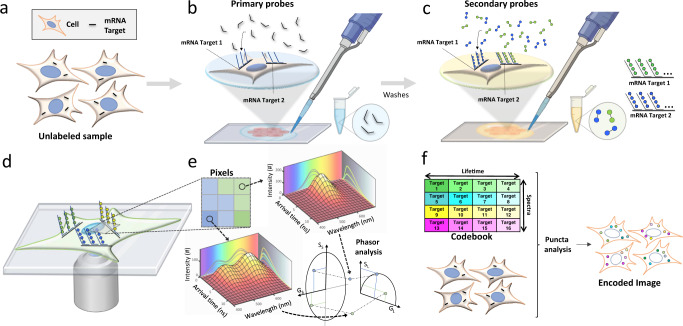
Fig. 1
Schematic of the MOSAICA approach for labeling and analysis of spectral and time-resolved components.
a Sample(s) can be fixed cells or tissues. RNA transcripts from genes of interest are targeted for detection. Protein targets can be stained too in mRNA and protein codetection. b Primary labeling pro...
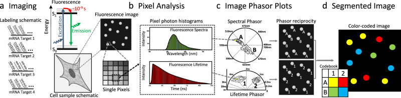
Fig. 2
Image and phasor analysis with spectrum and lifetime analysis in MOSAICA.
a As an example, four different probes are used to target the transcripts of four different genes. The fluorescence is collected using the spectral and Fluorescence Lifetime Imaging and Microscopy (FL...
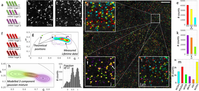
Fig. 3
Working example of combinatorial labelling of three mRNA targets with two probes.
a Transcripts of three different target genes are tagged using two probes with different spectra. Targets 1 and 3 are tagged each with one probe, Target 2 is tagged with both simultaneously. b , c The...
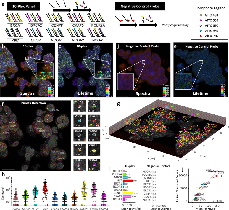
Fig. 4
Simultaneous 10-plex detection of transcripts for genes in colorectal cancer SW480 cells in a single round of labeling and imaging.
a 10 different gene transcripts are labeled with primary probes followed by respective and complementary fluorescent secondary probes. Each transcript is labeled with a combination of 2 out of 5 fluor...
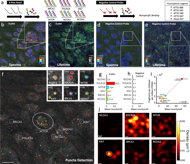
Fig. 5
Multiplexed mRNA detection in epidermis region of human skin melanoma FFPE tissue.
a 6 different types of gene transcripts were labeled with primary probes followed by respective and complementary fluorescent secondary probes. Each transcript was labeled with a combination of two di...
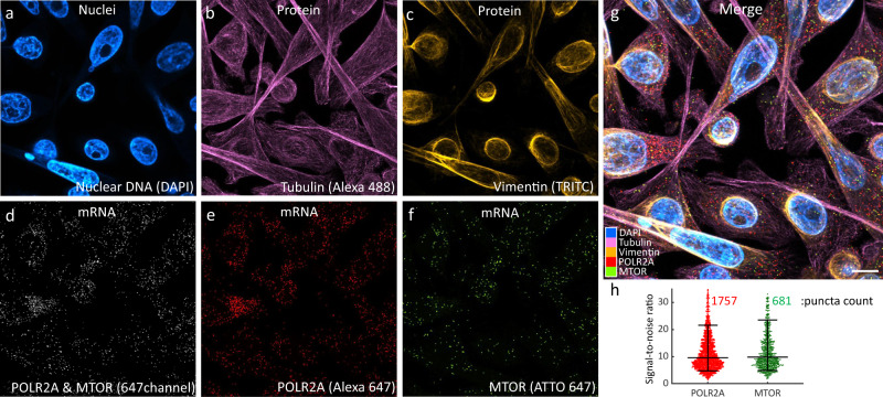
Fig. 6
Simultaneous 4-plex co-detection of protein and mRNA in colorectal cancer SW480 cells.
a Intensity imaging showing nuclei labeled with DAPI. b Intensity image showing Tubulin protein labeled with Alexa488. c Intensity image showing Vimentin protein labeled with TRITC. d Intensity image ...
Figure images are served from the NIH/NLM PubMed Central Open Access Subset or Europe PMC; copyright remains with the publishers and authors.
💬 Discussion
0 commentsNo comments yet. Be the first to start a discussion!
Leave a Comment