Abstract
Clathrin-mediated endocytosis is an essential cellular function in all eukaryotes that is driven by a self-assembled macromolecular machine of over 50 different proteins in tens to hundreds of copies. How these proteins are organized to produce endocytic vesicles with high precision and efficiency is not understood. Here, we developed high-throughput superresolution microscopy to reconstruct the nanoscale structural organization of 23 endocytic proteins from over 100,000 endocytic sites in yeast. We found that proteins assemble by radially ordered recruitment according to function. WASP family proteins form a circular nanoscale template on the membrane to spatially control actin nucleation during vesicle formation. Mathematical modeling of actin polymerization showed that this WASP nano-template optimizes force generation for membrane invagination and substantially increases the efficiency of endocytosis. Such nanoscale pre-patterning of actin nucleation may represent a general design principle for directional force generation in membrane remodeling processes such as during cell migration and division.
🔬 Techniques
🧬 Organisms
💻 Software
✨ Fluorophores
🧪 Sample Preparation
🏭 Microscope Brands
🧪 Reagent Suppliers
📷 Detectors
🔎 Objectives
🎨 Filters
💻 Software Details
💻 Code & Software
💾 Data Repositories
🏛️ Research Organizations (ROR)
Affiliated research institutions:
📋 Methods
Experimental Pipeline
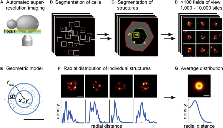
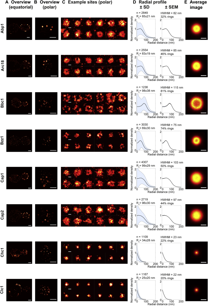
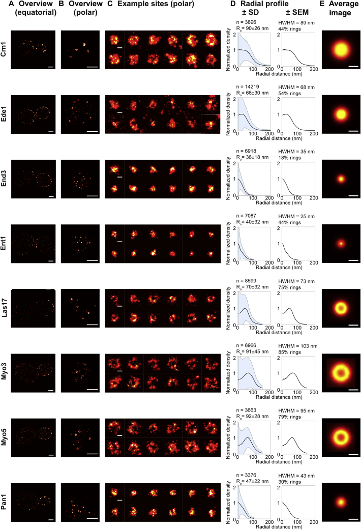
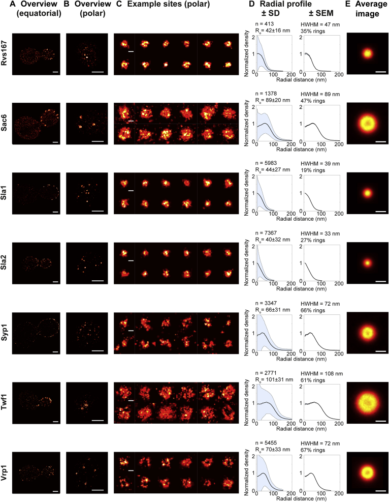
Here, we used single-molecule localization microscopy (SMLM, also called “(f)PALM” or “STORM”) ( Betzig et al., 2006 , Hess et al., 2006 , Rust et al., 2006 ) to image sites of clathrin-mediated endocytosis in budding yeast strains with single endocytic proteins endogenously tagged at their C termini with a photoswitchable fluorescent protein. We fixed the cells with formaldehyde, and then placed the focal plane on their underside, where endocytic invaginations are oriented perpendicularly to the focal plane ( Figure 1 A). Thereby we obtained two-dimensional (2D) projections of endocytic structures, which reveal the lateral distribution of proteins at endocytic sites. In these images, the distribution of endocytic proteins appeared as patches, rings, or irregular shapes ( Figures S1 , S2 , and S3 ). Figure 1 High-Throughput Superresolution Imaging of Endocytosis in Yeast (A) Fixed yeast cells expressing fluorescently tagged endocytic proteins were imaged using 2D high-throughput superresolution microscopy with the focal plane at the bottom of the cells. Images contain the 2D projection of the entire endocytic site in the membrane plane. (B–E) Cells (B) and endocytic sites were automatically segmented only in the center of cells (C) to avoid tilted structures. Individual endocytic sites (D) were analyzed by fitting a single geometric model (E) to determine center coordinates x 0 , y 0 , outer radius r out , and a rim with a thickness dr . The model accounts for the localization precision and describes both patch-like ( dr ≥ r out ) and ring-like ( dr < r out ) structures. (F) The radial density distribution around x 0 , y 0 was calculated for each site. (G) Using x 0 , y 0 individual sites were aligned by translation, and the average protein distribution and radial density profiles were calculated. Scale bars represent 100 nm. See also Figures S1 , S2 , and S3 and Table S1 . Figure S1 Overview of Imaged Endocytic Proteins (Part 1/3), Related to Figures 1 and 2 (A and B) Shown are superresolved images of cells where the focal plane was positioned on the midplane (A) and bottom (B) of the cells. (C) Shows example endocytic sites focused as in (B). (D) Shows average radial profiles. Shaded areas correspond to the standard deviation (left) or standard error of the mean (right). (E) Shows the average image. The number of sites, fraction of rings as obtained by the fit from the dr/r out values (see the STAR Methods for details), the half-maximum of radial profiles (HWHM), as well as the mean and standard deviation of the outer radius as obtained by the fit are indicated. Scale bars 1 μm (A and B) or 100 nm (C and E). Figure S2 Overview of Imaged Endocytic Proteins (Part 2/3), Related to Figures 1 and 2 (A–E) As in Figure S1 . Scale bars 1 μm (A and B) or 100 nm (C and E). Figure S3 Overview of Imaged Endocytic Proteins (Part 3/3), Related to Figures 1 and 2 (A–E) As in Figure S1 . Scale bars 1 μm (A and B) or 100 nm (C and E). Because endocytosis was arrested by fixation, the individual images provide snapshots of different endocytic time points. To sample the entire endocytic timeline with high statistical power, we automatically acquired and segmented superresolution images of many thousands of endocytic sites ( Figures 1 B–1D), quantitatively analyzed individual structures ( Figures 1 E and 1F), spatially aligned them by translation, and averaged them. We thereby generated density profiles of how each protein is on average distributed around the center of the endocytic site ( Figure 1 G), representing the average structural organization of endocytic proteins over their lifetime. Additionally, we determined how the distribution of four key endocytic proteins evolves during endocytosis.
Show full methods section
Experimental Pipeline
Here, we used single-molecule localization microscopy (SMLM, also called “(f)PALM” or “STORM”) ( Betzig et al., 2006 , Hess et al., 2006 , Rust et al., 2006 ) to image sites of clathrin-mediated endocytosis in budding yeast strains with single endocytic proteins endogenously tagged at their C termini with a photoswitchable fluorescent protein. We fixed the cells with formaldehyde, and then placed the focal plane on their underside, where endocytic invaginations are oriented perpendicularly to the focal plane ( Figure 1 A). Thereby we obtained two-dimensional (2D) projections of endocytic structures, which reveal the lateral distribution of proteins at endocytic sites. In these images, the distribution of endocytic proteins appeared as patches, rings, or irregular shapes ( Figures S1 , S2 , and S3 ). Figure 1 High-Throughput Superresolution Imaging of Endocytosis in Yeast (A) Fixed yeast cells expressing fluorescently tagged endocytic proteins were imaged using 2D high-throughput superresolution microscopy with the focal plane at the bottom of the cells. Images contain the 2D projection of the entire endocytic site in the membrane plane. (B–E) Cells (B) and endocytic sites were automatically segmented only in the center of cells (C) to avoid tilted structures. Individual endocytic sites (D) were analyzed by fitting a single geometric model (E) to determine center coordinates x 0 , y 0 , outer radius r out , and a rim with a thickness dr . The model accounts for the localization precision and describes both patch-like ( dr ≥ r out ) and ring-like ( dr < r out ) structures. (F) The radial density distribution around x 0 , y 0 was calculated for each site. (G) Using x 0 , y 0 individual sites were aligned by translation, and the average protein distribution and radial density profiles were calculated. Scale bars represent 100 nm. See also Figures S1 , S2 , and S3 and Table S1 . Figure S1 Overview of Imaged Endocytic Proteins (Part 1/3), Related to Figures 1 and 2 (A and B) Shown are superresolved images of cells where the focal plane was positioned on the midplane (A) and bottom (B) of the cells. (C) Shows example endocytic sites focused as in (B). (D) Shows average radial profiles. Shaded areas correspond to the standard deviation (left) or standard error of the mean (right). (E) Shows the average image. The number of sites, fraction of rings as obtained by the fit from the dr/r out values (see the STAR Methods for details), the half-maximum of radial profiles (HWHM), as well as the mean and standard deviation of the outer radius as obtained by the fit are indicated. Scale bars 1 μm (A and B) or 100 nm (C and E). Figure S2 Overview of Imaged Endocytic Proteins (Part 2/3), Related to Figures 1 and 2 (A–E) As in Figure S1 . Scale bars 1 μm (A and B) or 100 nm (C and E). Figure S3 Overview of Imaged Endocytic Proteins (Part 3/3), Related to Figures 1 and 2 (A–E) As in Figure S1 . Scale bars 1 μm (A and B) or 100 nm (C and E). Because endocytosis was arrested by fixation, the individual images provide snapshots of different endocytic time points. To sample the entire endocytic timeline with high statistical power, we automatically acquired and segmented superresolution images of many thousands of endocytic sites ( Figures 1 B–1D), quantitatively analyzed individual structures ( Figures 1 E and 1F), spatially aligned them by translation, and averaged them. We thereby generated density profiles of how each protein is on average distributed around the center of the endocytic site ( Figure 1 G), representing the average structural organization of endocytic proteins over their lifetime. Additionally, we determined how the distribution of four key endocytic proteins evolves during endocytosis.
STAR★Methods Key Resources Table
REAGENT or RESOURCE SOURCE IDENTIFIER Chemicals, Peptides, and Recombinant Proteins 4-Aminobenzoic acid Merck Cat#822312; CAS: 150-13-0 5-Fluoroorotic Acid Monohydrate Toronto Research Chemicals Cat#F595000; CAS: 220141-70-8 Adenine Sigma-Aldrich Cat#A8626; CAS: 73-24-5 Adenine hemisulfate salt Sigma-Aldrich Cat#A3159; CAS: 321-30-2 Ammonium Chloride Merck Cat#101145; CAS: 12125-02-9 anti-GFP nanobody conjugated to Alexa Fluor 647 Custom made N/A Bacto Agar BD Biocsciences Cat#214010 Bovine Serum Albumin Sigma-Aldrich Cat#A7030; CAS: 9048-46-8 Catalase from bovine liver Sigma-Aldrich Cat#C3155; CAS: 9001-05-2 Concanavalin A Sigma-Aldrich Cat#C2010; CAS: 11028-71-0 Cysteamine Sigma-Aldrich Cat#30070; CAS: 60-23-1 D-Galactose Serva Cat#22020; CAS: 59-23-4 D-Sorbitol Sigma-Aldrich Cat#S3889; CAS: 50-70-4 D(+)-Glucose monohydrate Merck Cat#104074; CAS: 14431-43-7 Deuterium Oxide (99.8%) euriso-top Cat#D216L-MPT; CAS: 7789-20-0 DMSO, anhydrous Sigma-Aldrich Cat#276855; CAS: 67-68-5 dNTP Mix ThermoFisher Scientific Cat#R0191 DTT Sigma-Aldrich Cat#43819; CAS: 3483-12-3 EDTA Merck Cat#108418: CAS: 6381-92-6 FastAP Thermosensitive Alkaline Phosphatase ThermoFisher Scientific Cat#EF0651 FastDigest BamHI ThermoFisher Scientific Cat#FD0054 FastDigest Nco I ThermoFisher Scientific Cat#FD0573 FastDigest SalI ThermoFisher Scientific Cat#FD0644 Formaldehyde solution about 37% Merck Cat#104003 Glucose Oxidase from Aspergillus niger Sigma-Aldrich Cat#49180; CAS: 9001-37-0 Glutamine Sigma-Aldrich Cat#P0380; CAS: 147-85-3 Glycine Sigma-Aldrich Cat#G7126; CAS: 56-40-6 Hydrochloric acid fuming 37% Merck Cat#100317 Hygromycin B Roth Cat#CP13; CAS: 31282-04-9 Image-iT FX Signal Enhancer ThermoFisher Scientific Cat# I36933 L-Alanine Sigma-Aldrich Cat#A7627; CAS: 56-41-7 L-Arginine Sigma-Aldrich Cat#A5006; CAS: 74-79-3 L-Asparagine Sigma-Aldrich Cat#A0884; CAS: 70-47-3 L-Aspartic Acid Sigma-Aldrich Cat#A9256; CAS: 56-84-8 L-Cysteine hydrochloride monohydrate Sigma-Aldrich Cat#C7880; CAS: 7048-04-6 L-Glutamic Acid Sigma-Aldrich Cat#G1251; CAS: 56-86-0 L-Histidine Sigma-Aldrich Cat#H8000; CAS: 71-00-1 L-Isoleucine Sigma-Aldrich Cat#I2752; CAS: 73-32-5 L-Leucine Sigma-Aldrich Cat#L8000; CAS: 61-90-5 L-Lysine monohydrochloride Sigma-Aldrich Cat#L5626; CAS: 657-27-2 L-Methionine Sigma-Aldrich Cat#M9625; CAS: 63-68-3 L-Phenylalanine Sigma-Aldrich Cat#P2126; CAS: 63-91-2 L-Proline Sigma-Aldrich Cat#P0380; CAS: 147-85-3 L-Serine Sigma-Aldrich Cat#S4500; CAS: 56-45-1 L-Threonine Sigma-Aldrich Cat#T8625; CAS: 72-19-5 L-Tryptophan Sigma-Aldrich Cat#T0254; CAS: 73-22-3 L-Tyrosine Sigma-Aldrich Cat#T3754; CAS: 60-18-4 L-Valine Sigma-Aldrich Cat#V0500; CAS: 72-18-4 Latrunculin A abcam Cat#ab144290; CAS: 76343-93-6 Lithium acetate dihydrate Sigma-Aldrich Cat#L6883; CAS: 6108-17-4 Magnesium Chloride Merck Cat#105833; CAS: 7791-18-6 MangoMix PCR Master Mix Bioline Cat#BIO-25033 Methanol Merck Cat#106009; CAS: 67-56-1 myo -Inositol Sigma-Aldrich Cat#I7508; CAS: 87-89-8 Nourseothricin Jena Bioscience Cat#AB-102; CAS: 96736-11-7 Pac I New England BioLabs Cat#R054S Peptone BD Biocsciences Cat#211677 Poly(ethylene glycol) 3350 Sigma-Aldrich Cat#P3640; CAS: 25322-68-3 Potassium Acetate Merck Cat#104820; CAS: 127-08-2 SNAP-Surface Alexa Fluor 647 New England BioLabs Cat#S9136S Sodium Chloride Merck Cat#106404; CAS: 7647-14-5 ssDNA Sigma-Aldrich Cat#D1626; CAS: 438545-06-3 Sucrose Sigma-Aldrich Cat#S0389; CAS: 57-50-1 T4 DNA Ligase ThermoFisher Scientific Cat#EL0011 TetraSpeck beads (0.1 μm) ThermoFisher Scientific Cat#T7279 Triton X-100 Sigma-Aldrich Cat#X100; CAS: 9002-93-1 Trizma base Sigma-Aldrich Cat#T1503; CAS: 77-86-1 Tryptone BD Biocsciences Cat#211705 Uracil Sigma-Aldrich Cat#U0750; CAS: 66-22-8 Velocity DNA Polymerase Bioline Cat#BIO-21098 Yeast Extract BD Biocsciences Cat#212750 Yeast Nitrogen Base w/o Amino Acids BD Biocsciences Cat#291940 α-D-Raffinose Serva Cat#34140; CAS: 17629-30-0 Experimental Models: Organisms/Strains S. cerevisiae MK0100 Kaksonen lab N/A S. cerevisiae MK0102 Kaksonen lab N/A A full list of strains is presented in Table S3 This paper N/A Recombinant DNA pFA6a-EGFP-HIS3MX6 Janke et al., 2004 N/A pJR58 pFA6a-mMaple-HIS3MX6 This paper N/A pMM02 pFA6a-mMaple-hphNT1 This paper N/A pJR40 pFA6a-SNAPf-HIS3MX6 This paper N/A pMaM173 Khmelinskii et al., 2011 N/A pMaM173-mMaple This paper N/A Software and Algorithms Blender 2.78 Blender Foundation https://www.blender.org/ Cytosim Nédélec and Foethke, 2007 https://github.com/nedelec/cytosim Fiji (ImageJ) Schindelin et al., 2012 http://fiji.sc/ MATLAB MathWorks https://www.mathworks.com/products/matlab.html Running Z-Projector Fiji plugin Nico Stuurman https://valelab4.ucsf.edu/∼nstuurman/IJplugins/Running_ZProjector.html SMAP (Single Molecule Analysis Platform) Ries lab https://github.com/jries/SMAP μManager Edelstein et al., 2010 https://micro-manager.org/ Other 160x NA 1.43 TIRF objective (HCX PL APO 160x/1.43 Oil CORR GSD) Leica Microsystems N/A 24 mm round glass coverslips (No. 1.5H) Marienfeld Cat#0117640 525/50 BrightLine single-band bandpass filter Semrock Cat#FF03-525/50-25 60x NA 1.49 TIRF objective Nikon N/A 640 LP dichroic mirror Chroma Cat#ZT640rdc 676/37 BrightLine single-band bandpass filter Semrock Cat#FF01-676/37-25 ET600/60 emission filter Chroma Cat#NC458462 Evolve512D EMCCD camera Photometrics N/A iChrome MLE-L laser box (405, 488, 561, 638 nm) Toptica Photonics N/A Ixon Ultra EMCCD camera Andor N/A LightHUB laser box (405, 488, 561, 638 nm) Omicron N/A Multimode fiber Thorlabs Cat#M105L02S-A Piezo objective positioner Physik Instrumente N/A PlasmaPrep2 plasma cleaner Gala Instrumente N/A Transmissive laser speckle reducer Optotune Cat#LSR-3005-17S-VIS Contact for Reagent and Resource Sharing Further information and requests for resources and reagents should be directed to and will be fulfilled by the Lead Contact, Jonas Ries ( jonas.ries@embl.de ).
Experimental Model and Subject Details
All yeast strains used in this study were derivatives of S. cerevisiae MKY0100 or MKY0102 (Kaksonen lab). Construction of the strains is described below and a complete list of the strains used in this study is given in Table S3 . Yeast cells were inoculated from single colonies on plates into 4 mL YPAD in a glass tube, and grown overnight at 30°C with shaking. The next morning, the culture was rediluted into 10 mL YPAD in a glass flask to OD 600 of 0.25, and grown for 3-4 more hours at 30°C for sample preparation, typically reaching OD 600 of 0.6-1.0. SLA1 and SLA2 deletion strains were incubated at 25°C and grown for longer times to reach the desired OD 600 , but otherwise prepared identically. For imaging of Latrunculin A arrested endocytic sites, cells were grown overnight in YPAD but diluted the next morning in SC-Trp to reduce the autofluorescent background for live cell experiments. Method Details Yeast strain creation Yeast strains expressing endocytic proteins tagged with mMaple ( McEvoy et al., 2012 ) or SNAP f tag ( Sun et al., 2011 ) at their C-termini were generated by homologous recombination using the PCR cassette system ( Janke et al., 2004 ) in the parental strains MKY0100, MKY0102, MKY0122, MKY1596 and MKY2832. Sla2 was tagged with GFP in a parental strain expressing Ede1-mMaple. Correct integration of the tag was validated by colony PCR and fluorescence microscopy. Tagging plasmids containing the coding sequences of mMaple or SNAP f tag were created by replacing the coding sequence of GFP in either pFA6a-EGFP-HIS3MX6 (for histidine auxotrophy as selectable marker) or pFA6a-GFP-hphNT1 (for hygromycin resistance as selectable marker) between the Sal I and Bam HI restriction sites. The plasmid pMaM173-mMaple for N-terminal tagging was derived in a similar way from pMaM173 by replacing the parts specific for sfGFP using the SalI, Nco I, Pac I and BamHI restriction sites. Las17-mMaple was mated with MKY0764 to obtain the SLA2 deletion with Las17-mMaple (JRY0040). JRY0038 was mated with MKY3247 to obtain the BBC1 deletion in Las17-mMaple (JRY0076). The SLA1 deletion with Las17-mMaple and Abp1-GFP (JRY0084) was generated by mating JRY0041 with MKY1596. For N-terminal tagging of Myo5, the protocol for seamless tagging was used ( Khmelinskii et al., 2011 ). Here, a DNA cassette containing the first 180 bp of mMaple, a selectable marker for the synthesis of uracil surrounded by two I- Sce I restriction sites and full-length mMaple is inserted into MKY1743 using homologous recombination. After correct integration of this cassette, the expression of I- Sce I is induced by cultivation on plates containing galactose. This leads to an excision of the selectable marker and repair of the resulting double strand break using the fragment of mMaple and full-length mMaple as templates. Successful removal of the cassette is tested by negative selection against the URA3 marker using a 5-FOA plate. Sample preparation for imaging 24 mm round glass coverslips were cleaned overnight in methanol/hydrochloric acid (50/50) while stirring. They were then rinsed repeatedly with water until the pH of the washing solution remained neutral. Subsequently, they were plasma cleaned for 5-10 min. A drop of 20 μL ConA solution (4 mg/mL in PBS) was added to each coverslip, and let incubate for 30 min in a sealed, humidified atmosphere to avoid evaporation. Then, the remaining liquid was removed and the coverslips were dried overnight at 37°C. Prior to the day of imaging, yeast cells were inoculated from single colonies on plates into 4 mL YPAD in a glass tube, and grown overnight at 30°C with shaking. The next morning, the culture was rediluted into 10 mL YPAD in a glass flask to OD 600 of 0.25, and grown for 3-4 more hours at 30°C for sample preparation, typically reaching OD 600 of 0.6-1.0. SLA1 and SLA2 deletion strains were incubated at 25°C and grown for longer times to reach the desired OD 600 , but otherwise prepared identically. Because endocytosis proceeds considerably faster than typical image acquisition times in SMLM, we chemically fixed the cells in order to obtain images with the highest possible spatial resolution ( Mund et al., 2014 ). For this, 2 mL of the culture were collected by centrifugation at 500 rcf. for 2.5 min, resuspended in 100 μL YPAD and pipetted on a ConA coated coverslip, which has been briefly rinsed with water. The cells were allowed to settle for 15 min in a humidified atmosphere to prevent evaporation, and protected from light. After settling, the coverslip was directly transferred into the freshly prepared fixation solution containing 4% (w/v) formaldehyde, 2% (w/v) sucrose in PBS. Fixation was allowed to proceed for 15 min at gentle orbital shaking. The coverslip was then incubated for 15 min in 100 mM NH 4 Cl in PBS to quench remaining aldehyde groups. Quenching was repeated once more, before the coverslip was washed 3 times 5 min in PBS. At this point, the sample was ready for single color superresolution imaging. For simultaneous dual-color imaging using mMaple and SNAP f tag ( Figures 4 A, 4C, and 5 F), samples were processed further. 300 μL of permeabilization solution (0.25% (v/v) Triton X-100, 50% (v/v) ImageIT FX, in PBS) were added to the coverslip with cells facing up, and the coverslip was slowly agitated on an orbital shaker. The gentle shaking dissociated loosely bound cells from the coverslip, reducing the background. Permeabilization and blocking was allowed to proceed for 30 min, before the coverslip was washed 3 times 5 min in PBS. The coverslip was then transferred face down on a drop of 100 μL staining solution (1 μM SNAP Surface Alexa Fluor 647, 1% (w/v) BSA, 1 mM DTT, 0.25% (v/v) Triton X-100, in PBS) on parafilm. After staining for 2h, the sample was washed 3 times 5 min in PBS. For the dual-color imaging of Ede1 and Sla2 ( Figure 3 E), GFP-tagged Sla2 was stained with nanobodies that are specific for GFP and are conjugated to Alexa Fluor 647 using sortase tagging. Yeast cells on a coverslip were fixed, permeabilized and blocked as described above. Subsequently, the coverslip was transferred face down on a drop of 100 μL nanobody staining solution (anti-GFP nanobody, 1% (w/v) BSA, 0.25% (v/v) Triton X-100, in PBS) on parafilm and incubated for 2 hr in the dark under a humidified atmosphere. After washing the coverslip 3 times for 5 min in PBS the sample was ready for simultaneous imaging of mMaple and Alexa Fluor 647. For imaging of Latrunculin A arrested endocytic sites, cells were grown overnight in YPAD but diluted the next morning in SC-Trp to reduce the autofluorescent background for live cell experiments. For live cell imaging, 200 μL of a log phase culture were mixed with 2 μL of 20 mM LatA in DMSO (f.c. 200 μM) and pipetted onto a ConA coated coverslip. After 15 min of incubation to let the cells settle and LatA take effect, the medium was replaced by 200 μL fresh SC-Trp supplemented with 200 μM LatA to further reduce background fluorescence. The arrested endocytic patches were imaged until they clustered too much to distinguish individual sites, which was typically 45 min. As comparison a sample with fixed LatA arrested cells was prepared. For this, 1 mL from the same culture was spun down, resuspended in 100 μL of SC-Trp, supplemented with 200 μM LatA and pipetted onto a ConA coated coverslip. After 10 min, 100 μL of 8% (w/v) formaldehyde in SC-Trp was added onto the coverslip and incubated for another 10 min. Subsequently, the sample was prepared as described above for single color sample preparation by fixation, quenching, and washing.
Superresolution imaging
Single-color superresolution imaging
All single-color superresolution images were acquired on a custom-built, fully automated microscope, which was built for stable long-term automated image acquisition, and featured homogeneous high power illumination as described previously ( Deschamps et al., 2016 ). The free-space output of a commercial LightHUB laser box with 405 nm, 488 nm, 561 nm and 638 nm laser lines was collimated, focused on a speckle reducer and coupled into a multimode fiber. The output of the fiber was then imaged into the sample to homogenously illuminate a circular area of ∼1000 μm 2 . Fluorescence was collected through a 160x NA 1.42 TIRF objective, filtered by a bandpass filter (for GFP: 525/50; for mMaple: 600/60), and focused onto an Evolve512D EMCCD camera. The z focus was optically stabilized by total internally reflecting an additional IR laser off the coverslip onto a quadrant photo diode, which was coupled into an electronic feedback loop with the piezo objective positioner. Z focus stability was typically better than 5 nm/h. All microscope components are controlled by a custom-written plugin for μManager ( Edelstein et al., 2010 ). For single-color superresolution imaging, samples were mounted in a D 2 O-based imaging buffer (50 mM Tris-HCl pH 8 in 95% D 2 O) to improve brightness ( Ong et al., 2015 ). After selection of a region of interest, the back focal plane was imaged to ensure that the immersion oil contained no air bubbles. Then, videos of typically 10,000-100,000 frames were acquired using 561 nm illumination at ∼10 kW/cm 2 in the specimen plane at 25 ms exposure times with an EM gain of 200. During the experiment, mMaple was sparsely photoconverted to its red state by 405 nm illumination, making sure that single non-overlapping PSFs were observed. Using an automated feedback loop, 405 nm laser power was adjusted to keep a constant number of localizations per frame throughout the experiment. When no more blinking was observed, the experiment was terminated.
Automated superresolution imaging
The sample was mounted in imaging buffer and subsequently sealed airtight using parafilm to prevent evaporation of the buffer. For each sample, we first focused on the midplane of yeast cells, and acquired several fields of view to get a qualitative impression about the number and distribution of endocytic sites in each strain. We then adjusted the focal plane to ∼300 nm above the coverslip in order to image endocytic sites at the bottom of the cells. Because endocytic invaginations grow perpendicular to the plasma membrane in yeast, with a small spread around the right angle ( Kukulski et al., 2012 , Picco et al., 2015 ), and our depth of field is more than 600 nm as determined from bead stacks, this allowed us to obtain two-dimensional projections of endocytic structures along their axis of invagination into the plane of the plasma membrane. Using μManager, a grid of 100-500 positions was defined around the center of the stage, with each position spaced 200 μm away in every direction from the next region of interest to avoid cross-excitation and activation of neighboring positions due to scattered laser light. For each grid position, a set of acquisitions was performed automatically, each with a pre-defined set of settings for laser intensities, lens, and filter positions. First, a blinking video was recorded as described above, which was automatically stopped once the 405 nm intensity reached a threshold value, indicating that all mMaple molecules have been imaged and bleached. Subsequently, an image of the back focal plane was recorded to check for air bubbles in the immersion oil. For some experiments, mMaple superresolution imaging was combined with diffraction-limited GFP imaging to obtain an additional, diffraction-limited reference signal. GFP has been previously shown to have no substantial cross-talk into the mMaple channel ( Puchner et al., 2013 ). For this, z stacks of ± 2 μm were recorded in 50 nm steps around the focal plane in the GFP channel after mMaple superresolution imaging was completed. Once all different types of acquisitions were completed for one grid position, the stage was moved to the next one. In between different positions, a waiting time of 15 s allowed for mechanical equilibration after stage movement. The measurement cycle was repeated until all positions were imaged, or the experiment was terminated manually.
Dual-color imaging
The dual-color images shown in Figures 4 and 5 were acquired on a custom-built microscope with single-mode fiber-based illumination, where the single-mode output of a commercial iChrome MLE laser box with 405 nm, 488 nm, 561 nm and 638 nm laser lines was collimated, focused on the back focal plane of a 60 x NA 1.49 TIRF objective, and adjusted for epi illumination. Fluorescence emission was laterally constricted by a slit, split using a 640 LP dichroic mirror, separately filtered by 600/60 (mMaple signal) and 676/37 (Alexa Fluor 647 signal) bandpass filters, and imaged on two parts of the camera chip of an Ixon Ultra EMCCD camera. Analogous to the setup described above, the z focus was optically stabilized. Samples were mounted in thiol-containing blinking buffer with an enzymatic oxygen scavenger (50 mM Tris pH 8, 10 mM NaCl, 10% (w/v) D-glucose, 35 mM cysteamine, 0.5 mg/mL glucose oxidase, 40 μg/mL catalase, in ∼90% D 2 O). After selection of a region of interest, the back focal plane was imaged to ensure that the immersion oil contained no air bubbles. Then, the sample was illuminated both with 561 nm and 640 nm light, and videos of typically 10,000-100,000 frames were acquired at 30 ms exposure times with an EM gain of 200. During the experiment, 405 nm laser intensity was automatically adjusted to keep a constant number of non-overlapping PSFs as described above. When no more blinking was observed, the experiment was terminated. Dual-color images shown in Figure 3 E were acquired on the microscope described under Single-color superresolution imaging with the following modifications: The signal of the 2 fluorophores was split using a 640 LP dichroic mirror, separately filtered by 600/60 and 676/37 bandpass filters, and imaged on two parts of the camera chip.
Data analysis
All data analysis was performed using a custom comprehensive analysis software framework, SMAP (“Superresolution Microscopy Analysis Platform”, unpublished data), which was developed in MATLAB.
Single molecule localization
For localization, peaks were detected in the raw images by smoothing, background subtraction using a wavelet filter, and non-maximum suppression. Peaks with intensities above a dynamically determined threshold were then localized by fitting a pixelated Gaussian function with a homogeneous photon background. Fitting of individual PSFs was highly parallelized by using a GPU-based algorithm of a maximum-likelihood estimator for data that is Poisson distributed ( Smith et al., 2010 ). All experiments were automatically fitted online during the acquisition. During automatic acquisitions, new experiments were automatically detected and subjected to localization.
Image reconstruction
All image reconstruction was done in SMAP. Localizations that were found in consecutive frames (a gap of 1 frame was allowed) within a circular range of 75 nm radius were grouped into a single localization. Localizations with a localization precision worse than 30 nm and a fitted PSF standard deviation larger than 175 nm were discarded. These cutoffs are loose, and retained the majority of localizations, but efficiently removed dim localizations resulting from autofluorescent background and out-of-focus events. All filtered localizations were plotted at their coordinates as normalized Gaussians with a standard deviation proportional to their localization precision. To increase visibility of very precisely localized events, a minimum Gaussian standard deviation of 6 nm was used. To equalize pixels with very high brightness, the contrast was adjusted to saturate 0.01%–0.1% of the brightest intensity values. To correct for sample drift during the image acquisition, localizations were sorted according to the frame in which they were detected and binned in ten time windows, for which individual superresolution images were calculated. Then, the pairwise image cross-correlation of all intermediate images with all others was calculated, and spline interpolation was used to calculate the lateral drift trajectory, which was then corrected for. Typically, we observed a lateral drift of 20-100 nm/h. Drift correction was not applied for very short experiments with less than 5000 frames or when the detected lateral drift was below 10 nm.
Dual-color image reconstruction
In our dual-color imaging, the signals from mMaple and Alexa Fluor 647 were imaged on two separate parts of the camera chip. To overlay both channels, we experimentally determined a transformation function using a calibration bead sample. For the bead sample, we diluted TetraSpeck beads 1:200 in 100 mM MgCl 2 on a glass coverslip. We imaged at least 1,000 beads in both channels, localized them, and calculated a projective transformation from their positions. The accuracy of this transformation was better than 10 nm, as judged by the standard deviation of individual bead positions. This transformation was subsequently used to transform the mMaple channel onto the Alexa Fluor 647 channel.
Analysis of endocytic structures Quality control of automated imaging
Datasets that were generated by automatic superresolution imaging typically consisted of 100 to 500 fields of view, and were first subjected to quality control. All individual back focal plane (BFP) images were inspected for air bubbles. If single BFPs showed bubbles, the corresponding fields of view were discarded. If multiple BFPs showed bubbles, the entire dataset was discarded. Subsequently, statistics from the individual superresolved images were compared. We analyzed the median localization precision, median fitted photon background, total number of localizations and number of frames for each experiment. If any of those parameters did not remain approximately constant over time, this indicated changes in the sample or imaging conditions, e.g., a change in salt concentration or pH due to buffer evaporation. In this case, the experiment was either entirely discarded, or only the first adequate fields of view were used.
Segmentation of cells and endocytic sites
Cells were segmented in the superresolved images by filtering the image with a large Gaussian blur, and detecting peaks above a user-defined threshold, which was adjusted so that all cells were segmented properly. To segment endocytic sites, the superresolved image of the cell was rendered with a pixel size of 200 nm and masked using a user-defined threshold, which was adjusted once for each endocytic protein corresponding to their different abundances. This mask roughly represented the boundary of the cell. Then, a convex hull was drawn around all localizations within this mask, and subsequently constricted by iteratively removing the points on the hull 3 times. The resulting convex hull faithfully enveloped the cellular signal. The convex hull was then shrunk by at least 30% to define the center bottom of the cell, where endocytic sites were then segmented as follows. To segment endocytic sites, the superresolved image was rendered with a pixel size of 100 nm. In the filtered image, peaks above a user-defined threshold were picked. This cutoff was adjusted once for each endocytic protein. To avoid closely juxtaposed sites an upper size limit was empirically set, and visually confirmed to not be too restrictive and to only exclude clear double-sites, and no big individual sites. The size range was adjusted once for each protein. For clathrin (Clc1 and Chc1), site segmentation was complicated by the fact that in yeast a major fraction of clathrin molecules are found at intracellular membrane compartments, which are often close to the plasma membrane. Thus, we cannot rule out that a minor part of the segmented structures are not actually endocytic sites, but comparably small intracellular compartments, which might confound the structural analysis. Endocytic sites in SLA1 and SLA2 deletion strains, in LatA arrested live cell experiments as well as in dual color experiments were picked manually. Geometric analysis of endocytic sites Superresolved images of individual endocytic sites were rendered with a pixel size of 3 nm, and fitted with a geometric model that describes the shape either as ring or as patch, where rings have a hole in their center, around which there is a rim of a certain thickness. Patches do not have holes. Both rings and patches are described by their outer radius r out and the rim thickness dr . Because of their central holes, rings have r out > dr , whereas patches have r out ≤ dr . The model is illustrated below and formally described in Equations 1 and 2 , where I(X, Y) is the pixelated image, x 0 , y 0 are the coordinates of the center, r out is the outer radius, dr is the rim thickness, and A is a scaling factor. To account for the expected localization precision, a Gaussian blur with σ = 15 nm is introduced. (1) f ( X , Y ) = A ( erf ( r o u t − R ( X , Y ) 2 σ ) − erf ( r o u t − d r − R ( X , Y ) 2 σ ) ) (2) R ( X , Y ) = ( X − x 0 ) 2 + ( Y − y 0 ) 2 (3) { d r , r o u t , x 0 , y 0 } = argmin d r , r o u t , x 0 , y 0 ( ∑ X , Y ( I ( X , Y ) − f ( X , Y ) ) 2 ) Least-squares fitting was then performed numerically as shown in Equation 3 . We then calculated the radial distribution of the localizations around the fitted center coordinates to obtain the radial profile of individual endocytic sites. As we used a low threshold during automatic site segmentation to avoid biases from overly stringent segmentation, the dataset contained a comparably small set of structures with a low number of localizations and a small size on the order of the resolution. Because these structures were too small to obtain geometric information, we excluded structures with outer radii below 30 nm and below 30 localizations, i.e., with less than approximately 10 mMaple proteins, from the analysis. Because structures in the coat and scission modules (Clc1, Chc1, End3, Ent1, Pan1, Rvs167, Sla1, Sla2) mostly formed small structures, we only excluded structures with less than 30 localizations, and did not apply a size threshold. We then aligned the superresolution images and radial profiles of all endocytic sites by their center coordinates, and calculated the average images and radial profiles. Proteins of the actin module (Abp1, Arc18, Cap1, Cap2, Crn1, Sac6, Twf1) on average assembled into large structures (outer radius > 80 nm) with a slight minimum in the center of their radial profiles (density at the center is more than 80% of the maximum intensity). Because our images acquired in the equatorial plane ( Figure 5 ) show that the actin network occupies a large, hemispherical volume around the endocytic site, which agrees with previous reports using electron microscopy ( Kukulski et al., 2012 ), we classified these structures as dome-shaped. For dual-color bottom-view images ( Figures 3 and 4 ), both colors were analyzed analogously. In the geometric fit, both structures were fitted with common center coordinates ( Figure 4 ), or aligned by the fitted center coordinates of Sla2 ( Figure 3 ). To quantify GFP intensity corresponding to superresolved endocytic sites ( Figures 3 , 4 , and 5 ), we first calculated a maximum intensity projection of the 7 z stack slices around the focal plane. The projected images were corrected for chromatic aberrations between the GFP and mMaple channels using a transformation that was pre-determined using TetraSpeck beads, as described above. The background was calculated using a wavelet filter of level 3, and subtracted from the transformed images. For each endocytic site, the corresponding GFP intensity was determined by fitting the GFP image with three Gaussians: a first one fixed at the center coordinate of the superresolved site, and a second and third one with variable centers at least 350 nm away from the first one and each other to account for potential partial overlap of the diffraction-limited signals from proximal sites, which occurred frequently. If a site was entirely isolated, the amplitude of the second and third Gaussians were negligibly low. To avoid artificially high fitted GFP intensities that result from overlapping GFP signals from more than 2 sites, as was the case mostly in small buds, we excluded endocytic sites from the analysis where the fitted GFP intensity typically was more than 1.5 times the 80 th percentile of GFP intensities, which we empirically determined to faithfully exclude the highest GFP intensities. Eventually, we binned sites by their corresponding normalized GFP intensities into a bin with “no GFP” containing all sites with a normalized intensity < 0.1 times the 80 th percentile of GFP intensities, and three same-sized bins “low GFP,” “medium GFP” and “high GFP” containing equal share of the remaining sites sorted by GFP intensity.
Analysis of dual-color side-view images
Endocytic sites were segmented and rotated manually so that the direction of endocytosis is oriented upward. Then, the structures from both channels were segmented by thresholding and masking. For both channels, localizations were projected on the axis of endocytosis, and centroid and quantiles of the distribution along this axis were calculated. Endocytic sites were then aligned at the bottom by the 5 th percentile of the Las17 localizations, laterally aligned manually, and sorted by increasing Abp1 centroid position. The dual color images were rendered, and running window averages were calculated in Fiji using the Running Z-Projector plugin using ‘Average intensity’ and ‘window size 7’. We then compared the resulting averages to time-resolved outer boundaries of the actin network, that were determined as ribosome exclusion zones by CLEM ( Kukulski et al., 2012 ). Using the centroid distances from Picco et al. (2015) , we determined that the first of the running window averages corresponds approximately to −7 s, and that the last average corresponds to approximately 1 s. We assumed that the remaining frames are equally spaced in between, and manually overlaid the respective exclusion zone shapes from Figure 7 of Kukulski et al. (2012) , using the bottom of Las17 to align the membrane. Simulation of actin polymerization in Cytosim In brief, the Brownian dynamics simulation contains actin filaments assembled into a 3D network producing forces on the membrane. Filaments are nucleated by Arp2/3 complexes and connected by crosslinkers. The membrane invagination is represented by a movable object of constant shape, to which some actin filaments are bound via connectors mimicking Sla2/Ent1 proteins. All objects diffuse within a cylindrical volume built around an active patch on the plasma membrane, and may associate stochastically upon collision. The mechanical equilibrium of the network is simulated using overdamped Langevin dynamics ( Nédélec and Foethke, 2007 ), thus including Brownian motion and elasticity of the network. Chemical association/dissociations between the components, and filament assembly, are simulated stochastically following a modified Gillespie algorithm, which includes the effect that forces may have on the reaction rates. We describe the elements and methods of simulations in more details below. Filament mechanics Actin is modeled as slender elastic beams of rigidity κ, hence with a persistence length l p = κ / k B T , where k B T is the thermal energy, κ = 0.08 pNμm 2 ( Gittes et al., 1993 ) and thus l p ≈20 μm. The filaments are represented as strings of points separated by a distance s = 5.5 nm, and bending rigidity promotes the alignment of these points ( Nédélec and Foethke, 2007 ). For simplicity, actin filaments are not helical, i.e., they are cylindrical with complete rotational symmetry around their central axis, although they are displayed as helices on the figures for increased realism. Actin steric interactions The model includes steric interaction between actin filaments: two filaments located at a distance d repel each other if d 80 nm) with a slight minimum in the center of their radial profiles (density at the center is more than 80% of the maximum intensity). Because our images acquired in the equatorial plane ( Figure 5 ) show that the actin network occupies a large, hemispherical volume around the endocytic site, which agrees with previous reports using electron microscopy ( Kukulski et al., 2012 ), we classified these structures as dome-shaped. For dual-color bottom-view images ( Figures 3 and 4 ), both colors were analyzed analogously. In the geometric fit, both structures were fitted with common center coordinates ( Figure 4 ), or aligned by the fitted center coordinates of Sla2 ( Figure 3 ). To quantify GFP intensity corresponding to superresolved endocytic sites ( Figures 3 , 4 , and 5 ), we first calculated a maximum intensity projection of the 7 z stack slices around the focal plane. The projected images were corrected for chromatic aberrations between the GFP and mMaple channels using a transformation that was pre-determined using TetraSpeck beads, as described above. The background was calculated using a wavelet filter of level 3, and subtracted from the transformed images. For each endocytic site, the corresponding GFP intensity was determined by fitting the GFP image with three Gaussians: a first one fixed at the center coordinate of the superresolved site, and a second and third one with variable centers at least 350 nm away from the first one and each other to account for potential partial overlap of the diffraction-limited signals from proximal sites, which occurred frequently. If a site was entirely isolated, the amplitude of the second and third Gaussians were negligibly low. To avoid artificially high fitted GFP intensities that result from overlapping GFP signals from more than 2 sites, as was the case mostly in small buds, we excluded endocytic sites from the analysis where the fitted GFP intensity typically was more than 1.5 times the 80 th percentile of GFP intensities, which we empirically determined to faithfully exclude the highest GFP intensities. Eventually, we binned sites by their corresponding normalized GFP intensities into a bin with “no GFP” containing all sites with a normalized intensity < 0.1 times the 80 th percentile of GFP intensities, and three same-sized bins “low GFP,” “medium GFP” and “high GFP” containing equal share of the remaining sites sorted by GFP intensity.
Analysis of dual-color side-view images
Endocytic sites were segmented and rotated manually so that the direction of endocytosis is oriented upward. Then, the structures from both channels were segmented by thresholding and masking. For both channels, localizations were projected on the axis of endocytosis, and centroid and quantiles of the distribution along this axis were calculated. Endocytic sites were then aligned at the bottom by the 5 th percentile of the Las17 localizations, laterally aligned manually, and sorted by increasing Abp1 centroid position. The dual color images were rendered, and running window averages were calculated in Fiji using the Running Z-Projector plugin using ‘Average intensity’ and ‘window size 7’. We then compared the resulting averages to time-resolved outer boundaries of the actin network, that were determined as ribosome exclusion zones by CLEM ( Kukulski et al., 2012 ). Using the centroid distances from Picco et al. (2015) , we determined that the first of the running window averages corresponds approximately to −7 s, and that the last average corresponds to approximately 1 s. We assumed that the remaining frames are equally spaced in between, and manually overlaid the respective exclusion zone shapes from Figure 7 of Kukulski et al. (2012) , using the bottom of Las17 to align the membrane. Simulation of actin polymerization in Cytosim In brief, the Brownian dynamics simulation contains actin filaments assembled into a 3D network producing forces on the membrane. Filaments are nucleated by Arp2/3 complexes and connected by crosslinkers. The membrane invagination is represented by a movable object of constant shape, to which some actin filaments are bound via connectors mimicking Sla2/Ent1 proteins. All objects diffuse within a cylindrical volume built around an active patch on the plasma membrane, and may associate stochastically upon collision. The mechanical equilibrium of the network is simulated using overdamped Langevin dynamics ( Nédélec and Foethke, 2007 ), thus including Brownian motion and elasticity of the network. Chemical association/dissociations between the components, and filament assembly, are simulated stochastically following a modified Gillespie algorithm, which includes the effect that forces may have on the reaction rates. We describe the elements and methods of simulations in more details below. Filament mechanics Actin is modeled as slender elastic beams of rigidity κ, hence with a persistence length l p = κ / k B T , where k B T is the thermal energy, κ = 0.08 pNμm 2 ( Gittes et al., 1993 ) and thus l p ≈20 μm. The filaments are represented as strings of points separated by a distance s = 5.5 nm, and bending rigidity promotes the alignment of these points ( Nédélec and Foethke, 2007 ). For simplicity, actin filaments are not helical, i.e., they are cylindrical with complete rotational symmetry around their central axis, although they are displayed as helices on the figures for increased realism. Actin steric interactions The model includes steric interaction between actin filaments: two filaments located at a distance d repel each other if d
📊 Figures
Figureu00a01
High-Throughput Superresolution Imaging of Endocytosis in Yeast (A) Fixed yeast cells expressing fluorescently tagged endocytic proteins were imaged using 2D high-throughput superresolution microscopy...
Figureu00a0S1
Overview of Imaged Endocytic Proteins (Part 1/3), Related to Figures 1 and 2 (A and B) Shown are superresolved images of cells where the focal plane was positioned on the midplane (A) and bottom (B) o...
Figureu00a0S2
Overview of Imaged Endocytic Proteins (Part 2/3), Related to Figures 1 and 2 (Au2013E) As in Figureu00a0S1 . Scale bars 1u00a0u03bcm (A and B) or 100u00a0nm (C and E).
Figureu00a0S3
Overview of Imaged Endocytic Proteins (Part 3/3), Related to Figures 1 and 2 (Au2013E) As in Figureu00a0S1 . Scale bars 1u00a0u03bcm (A and B) or 100u00a0nm (C and E).
Figureu00a02
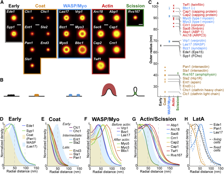
Average Radial Distribution of 23 Proteins in the Endocytic Machinery (A) Endocytic proteins form very diverse structures. Shown are the average images for 23 endocytic proteins (for a description, se...
Figureu00a0S4
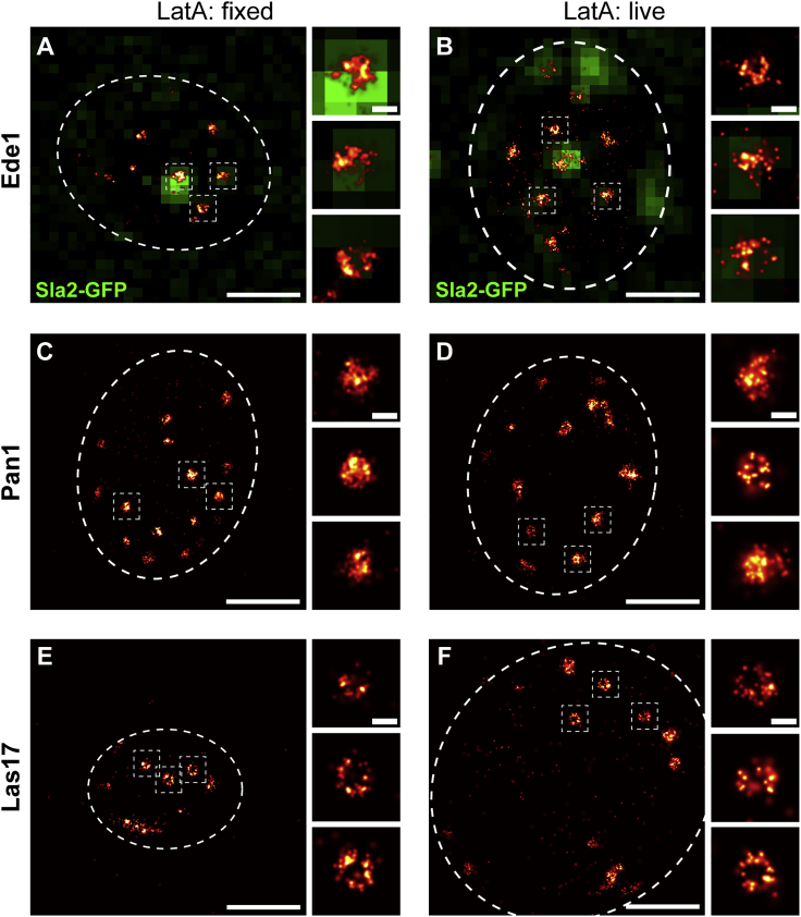
Ede1, Pan1, and Las17 Structures after Latrunculin A Treatment, Related to Figureu00a02 H (Au2013F) Shown are images of fixed (A, C, and E) and living (B, D, and F) cells, where endocytic sites have b...
Figureu00a03
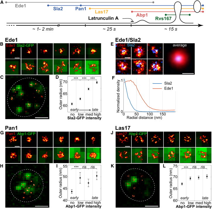
Structural Rearrangements of Key Proteins during Endocytosis (A) Strategy: Staging of endocytosis by combining superresolution imaging with diffraction-limited imaging of Sla2, Abp1, and Rvs167, which...
Figureu00a0S5
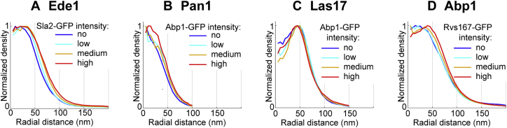
Average Radial Profiles of Ede1, Pan1, Las17, and Abp1 Staged Using Diffraction-Limited Timing Markers, Related to Figures 3 and 5 Average radial profiles of (A) Ede1-mMaple staged by Sla2-GFP, (B) Pa...
Figureu00a04
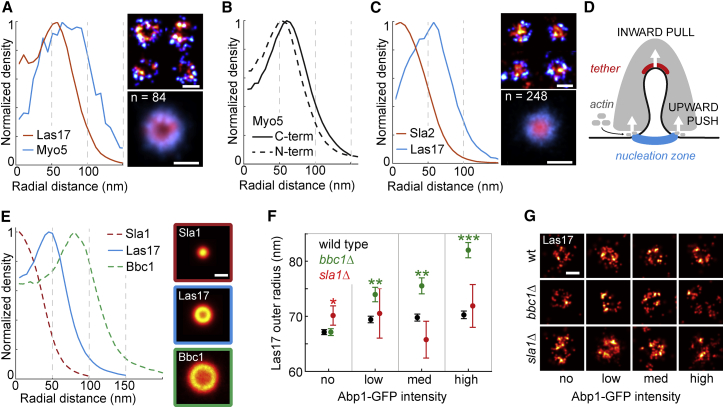
WASP Forms a Nano-Template for Actin Nucleation at the Membrane Base (A) Dual-color superresolution images of Las17-mMaple and Myo5-SNAP at individual endocytic sites, and average. (B) Radial profiles...
Figureu00a0S6
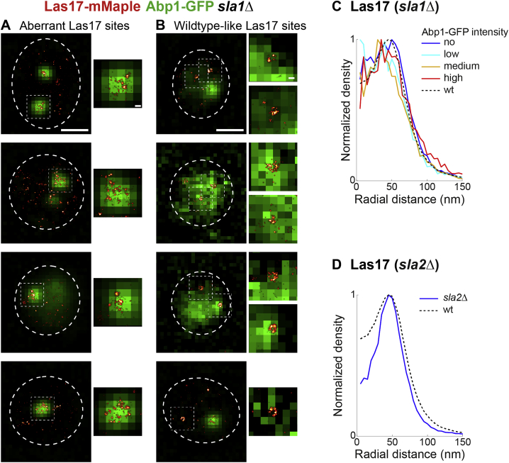
Las17 Structures in sla1u0394 Cells, Related to Figureu00a04 (A and B) SLA1 deletion leads to strong changes in Las17 structures. Shown are example sla1u0394 cells expressing Las17-mMaple and Abp1-GFP...
Figureu00a05
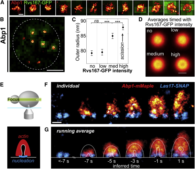
The Actin Network Emanates from the WASP Nucleation Zone (A and B) Abp1 in superresolution overlaid with diffraction-limited Rvs167-GFP as timing marker for vesicle scission at individual sites (A) an...
Figureu00a0S7
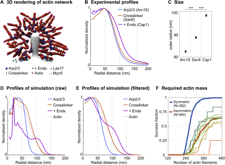
Potential Organization of Actin Filaments, Related to Figureu00a06 (A) Illustration of a thin slice through an endocytic actin network. (B and C) The experimental radial profiles (B) and mean outer ra...
Figureu00a06
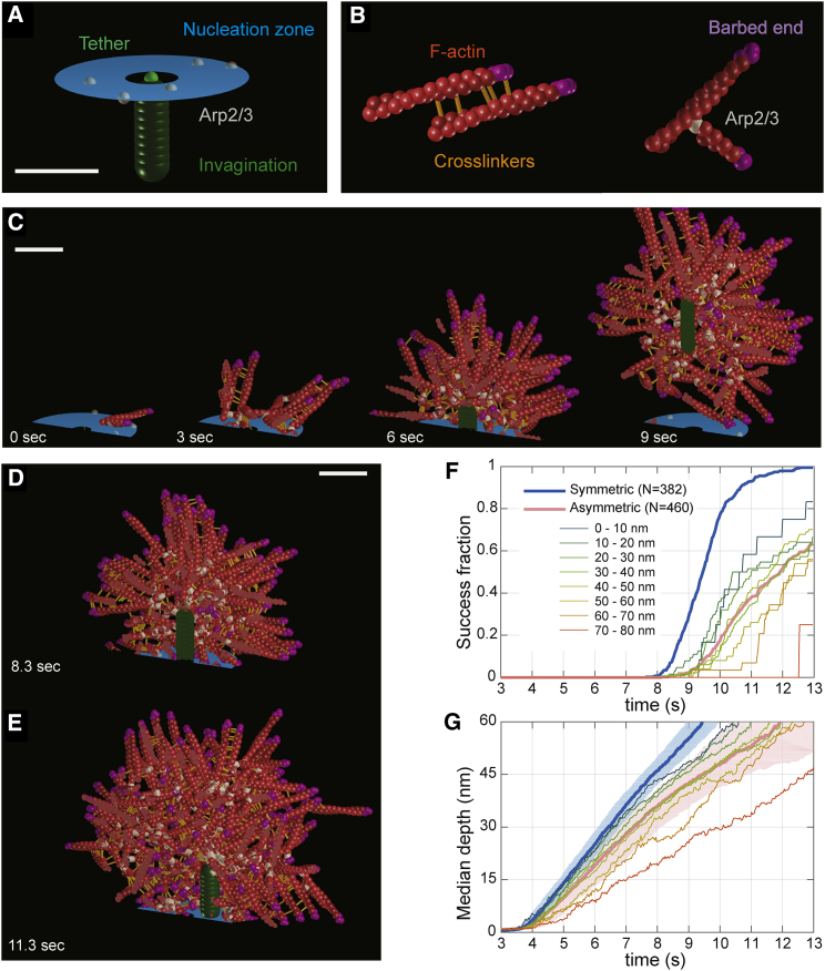
Simulations of the Actin Network at Endocytic Sites Using Cytosim (A and B) Initial configuration of the simulation (A) and overview of simulated elements (B). (C) Time series of a representative simu...
Figureu00a07
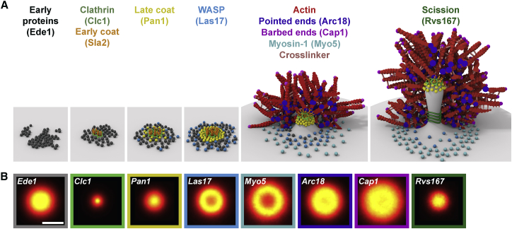
The Endocytic Machinery Assembles via Peripheral Binding (A) Schematic representation of the assembly of the endocytic machinery (for description, see text). (B) Representative radial averages of endo...
Figure images are served from the NIH/NLM PubMed Central Open Access Subset or Europe PMC; copyright remains with the publishers and authors.
💬 Discussion
0 commentsNo comments yet. Be the first to start a discussion!
Leave a Comment