Abstract
The two Condensin complexes in human cells are essential for mitotic chromosome structure. We used homozygous genome editing to fluorescently tag Condensin I and II subunits and mapped their absolute abundance, spacing, and dynamic localization during mitosis by fluorescence correlation spectroscopy (FSC)-calibrated live-cell imaging and superresolution microscopy. Although ∼35,000 Condensin II complexes are stably bound to chromosomes throughout mitosis, ∼195,000 Condensin I complexes dynamically bind in two steps: prometaphase and early anaphase. The two Condensins rarely colocalize at the chromatid axis, where Condensin II is centrally confined, but Condensin I reaches ∼50% of the chromatid diameter from its center. Based on our comprehensive quantitative data, we propose a three-step hierarchical loop model of mitotic chromosome compaction: Condensin II initially fixes loops of a maximum size of ∼450 kb at the chromatid axis, whose size is then reduced by Condensin I binding to ∼90 kb in prometaphase and ∼70 kb in anaphase, achieving maximum chromosome compaction upon sister chromatid segregation.
🔬 Techniques
🔭 Microscopes
🧬 Organisms
💻 Software
✨ Fluorophores
🧪 Sample Preparation
🔬 Cell Lines
🏭 Microscope Brands
🧪 Reagent Suppliers
📷 Detectors
🔎 Objectives
💻 Software Details
💻 Code & Software
💾 Data Repositories
🏛️ Research Organizations (ROR)
Affiliated research institutions:
📋 Methods
Cell culture
HK cells were obtained from S. Narumiya (Kyoto University, Kyoto, Japan) and grown in 1× high-glucose DMEM (41965039; Thermo Fisher Scientific) supplemented with 10% (vol/vol) FBS (10270106; Thermo Fisher Scientific; qualified, European Union approved, and South American origin), 100 U/ml penicillin-streptomycin (15140122; Thermo Fisher Scientific), 2 mM l -glutamine (25030081; Thermo Fisher Scientific), and 1 mM sodium pyruvate (11360070; Thermo Fisher Scientific) at 37°C and 5% CO 2 in cell culture dishes (Thermo Fisher Scientific) in a cell culture incubator. Cells were passaged every 2–3 d by trypsinization (Trypsin-EDTA [0.05%] and phenol red [25300054; Thermo Fisher Scientific]) at a confluency of 80–90%. Cells were confirmed to be mycoplasma free on a regular basis.
Cell line generation
HK cells were used for genome editing to express endogenously tagged proteins of interest (POIs). For tagging SMC4 at the C terminus and CAP-H at the N terminus with mEGFP, zinc finger nucleases (ZFNs) containing DNA binding sequences listed in Table S1 were purchased from Sigma-Aldrich. The donor plasmids consisted of the mEGFP cDNA sequence flanked by left and right homology arms listed in Table S2. ZFN pairs and the donor plasmids were transfected into HK cells as described by Mahen et al. (2014) and Koch et al. (2018) . For tagging CAP-D2 and CAP-D3 ( Wutz et al., 2017 ) at the C terminus, CAP-H and CAP-H2 at the C terminus, and CAP-H2 at the N terminus ( Cai et al., 2017 ) with mEGFP, paired CRISPR/Cas9D10A nickases were used. The design of guide RNAs (gRNAs) was performed as described by Otsuka et al. (2016) and Koch et al. (2018) (gRNAs listed in Table S1) and transfected together with donor plasmids (donor plasmids listed in Table S2) as described by Otsuka et al. (2016) and Koch et al. (2018) . For SMC4 and CAP-D2, only heterozygous clones were achieved after the first round of genome editing. Thus, after confirming by Sanger sequencing that the nontagged alleles were not mutated, a second round of genome editing identical to the first round was performed on top of a heterozygous clone, resulting in homozygous clones. The double-endogenously tagged cell line HK CAP-H2–mEGFP CAP-H–Halo was generated by using the homozygous HK CAP-H2–mEGFP clone as a parental cell line and performing genome editing based on the paired CRISPR/Cas9 D10A nickase approach (gRNAs listed in Table S1; donor plasmids listed in Table S2). All genome-edited cell lines were confirmed to be mycoplasma free on a regular basis. The tagging strategy was designed so that all Condensin isoforms could be tagged in the C-terminally mEGFP-tagged SMC4, CAP-D2, CAP-D3, and CAP-H cell lines. For CAP-H2, one theoretically predicted but not experimentally detected isoform could not be tagged in the C-terminally mEGFP-tagged cell line, but all isoforms could be tagged in the N-terminally mEGFP-tagged cell line. FCS-calibrated imaging of metaphase cells did not reveal a significant difference between the abundance of CAP-H2 proteins on metaphase chromosomes between N- and C-terminally tagged clones (see Fig. S2 G; two-sided Kolmogorov-Smirnov test; P = 0.1732 comparing data from eight C-terminally tagged clones, n = 81 cells, and five N-terminally tagged clones, n = 41 cells). Thus, C-terminally mEGFP-tagged clones for all Condensin subunits were used throughout this study apart from Fig. S2 (F and G), which shows data from both C- and N-terminally tagged CAP-H and CAP-H2 clones, respectively. Cell line validation Junction PCR, Southern blotting (SB), Western blotting (WB), confocal microscopy, mitotic timing analysis, and Sanger sequencing All single- and double-endogenously tagged cell lines were validated as described by Mahen et al. (2014) , Otsuka et al. (2016) , and Koch et al. (2018) by performing junction PCRs to test for integration and homozygosity (primers listed in Table S3), SB analysis with endogenous and GFP probes (and a Halo probe for double-tagged cell lines) to test for homozygosity, local genome rearrangements and additional integrations of the GFP or Halo donors (probes listed in Table S5), WB analysis to test for the expression of homozygously tagged proteins and absence of free GFP expression (ABs listed in Table S4), confocal microscopy to test for correct localization of the tagged proteins, widefield time-lapse microscopy and automated classification into mitotic phases ( Held et al., 2010 ) to confirm that mitotic timing (from prophase to anaphase onset) was not perturbed, and Sanger sequencing. To confirm the correct localization of Halo-tagged CAP-H in the double-endogenously tagged cell line, cells were stained with 100 nM Halo Tag TMR ligand (G8251; Promega) in prewarmed complete medium for 10 min at 37°C and 5% CO 2 and washed three times with prewarmed 1× PBS (homemade) followed by changing to imaging medium (CO 2 -independent imaging medium [custom order based on 18045070 from Thermo Fisher Scientific; without phenol red] supplemented with 20% [vol/vol] FBS [10270106; Thermo Fisher Scientific], 2 mM l -glutamine [25030081; Thermo Fisher Scientific], and 1 mM sodium pyruvate [11360070; Thermo Fisher Scientific]) and then incubated for 30 min at 37°C in the microscope incubation chamber before confocal microscopy as described by Koch et al. (2018) . In addition, coimmunoprecipitation against the GFP tag was performed for all selected single-homozygously mEGFP-tagged cell lines (HK 2× ZFN SMC4-mEGFP 82_68, HK 2× CRISPR CAP-D2–mEGFP 272_78, HK CRISPR CAP-D3–mEGFP 16, HK ZFN mEGFP–CAP-H 9, HK CRISPR CAP-H–mEGFP 86, HK CRISPR mEGFP–CAP-H2 1, HK CRISPR CAP-H2–mEGFP 67, and HK CRISPR CAP-H2–mEGFP 67 CRISPR CAP-H–Halo 29) to confirm the assembly of Condensin subunits into pentameric complexes (ABs listed in Table S4; for details, see next section). Anti-GFP IP and WB against Condensin subunits GFP–Trap A beads (gta-20; ChromoTek) were used to pull down mEGFP-tagged proteins in HK cell extracts. Cells grown to 80–90% confluence were harvested either as an asynchronously cycling population or after 18 h incubation with 330 nM nocodazole (Noc; 48792; Merck) to yield a mitotically arrested cell population. Cell pellets were lysed in the following lysis buffer: 10% glycerol (104093; Merck), 1 mM DTT (D-9779; Sigma-Aldrich), 0.15 mM EDTA (324503; Merck), 0.5% Triton X-100 (T8787; Sigma-Aldrich), one tablet of cOmplete EDTA protease inhibitor (11873580001; Roche), and one tablet PhosSTOP (04906837001; Roche). Lysis was performed on ice for 30 min, and the suspension was centrifuged at 13,000 rpm and 4°C for 10 min. The protein concentrations of the cell extracts were determined by protein assay (500-0006; Bio-Rad Laboratories), and 400 µg of total protein was used for IP. GFP–Trap A beads were washed twice with 1× PBS (homemade) and used at 1:1 dilution in PBS. 400 µg of total protein extracts were diluted 1:1 with PBS and incubated with the diluted GFP–Trap A beads at 4°C for 1 h. After the incubation, SN samples were taken, and the beads were washed twice with lysis buffer at 1:1 dilution with PBS. After two additional washing steps with PBS, 20 µl 4× NuPAGE LDS sample buffer (NP0008; Thermo Fisher Scientific) supplemented with 100 µM DTT was added to the beads and incubated at 65°C for 5 min to elute the protein from the beads. Input (IN), SN, and eluate (IP) samples were taken for WB against tagged and untagged subunits of the Condensin complexes (ABs listed in Table S4). FCS-calibrated confocal time-lapse imaging (sample preparation, FCS-calibrated confocal time-lapse imaging, data processing, and analysis) Samples for FCS-calibrated confocal time-lapse imaging were prepared as described by Cai et al. (2017) and Politi et al. (2018) . In brief, 2 × 10 4 cells that had been passaged the day before were seeded into individual chambers of a Nunc eight-well LabTek chambered coverglass (1.0; 155411; Thermo Fisher Scientific) and incubated overnight (ON) at 37°C and 5% CO 2 in a cell culture incubator. 2 h before imaging, the medium was changed to imaging medium (see the first subsection of Cell line validation) containing 50 nM SiR-DNA (SC007; Spirochrome; Lukinavičius et al., 2015 ) and 3.3 µM of 500-kD dextran (D7144; Thermo Fisher Scientific) labeled with Dy481XL (481XL-00; Dyomics; Dextran-Dy481XL was produced in house). FCS-calibrated confocal time-lapse imaging was performed as described by Cai et al. (2017) and Politi et al. (2018) (Fig. S1, D–H). FCS measurements of a 50-nM fluorescent dye solution of Alexa Fluor 488 (A20000; Thermo Fisher Scientific) in double-distilled H 2 O were performed to estimate the confocal volume. FCS measurements in both the nucleus and the cytoplasm of WT cells not expressing mEGFP were performed to determine background fluorescence and background photon counts. FCS measurements in both the nucleus and the cytoplasm of WT interphase cells expressing free mEGFP as well as interphase cells homozygously expressing an mEGFP-tagged Condensin subunit were performed to estimate an experiment-specific calibration factor that was used to transform mEGFP fluorescence into mEGFP concentration (Fig. S1 G). Prophase cells expressing an mEGFP-tagged Condensin subunit were automatically detected in low-resolution imaging mode based on the DNA staining (SiR-DNA) using CellCognition ( Held et al., 2010 ). Upon recognition of a prophase cell, high-resolution time-lapse imaging of this cell through mitosis was triggered. Hereby, a z stack covering the whole volume of the cell was acquired every 1.5 min for a total of 60 min in the mEGFP (mEGFP-tagged Condensin subunit), SiR-DNA (DNA), Dextran-Dy481XL (regions outside cells), and transmission channels. After each mitotic time lapse, one of the two daughter nuclei was detected, and six FCS measurements were acquired, three each inside and outside the nucleus, and used in addition to the interphase measurements for establishing the FCS calibration curve to transform mEGFP fluorescence intensities in each z stack of a mitotic time-lapse video into protein concentrations. A 3D segmentation pipeline was used to detect and track cells through mitosis as well as to reconstruct chromosomal and cell surfaces from the SiR-DNA and Dextran-Dy481XL channels, respectively ( Cai et al., 2017 ). To compensate for the variation of mitotic progression between individual cells, a mitotic standard time was computed based on geometric features of chromosomes, and each cell was aligned to this mitotic standard time of 60 min ( Cai et al., 2017 ). FCS data processing, generation of calibrated images, and data analysis to create cellular protein concentration and number maps (for details, please refer to the Estimation of protein numbers from FCS-calibrated images section) including a multistep quality control pipeline were performed as described by Wachsmuth et al. (2015) , Cai et al. (2017) , and Politi et al. (2018) .
Show full methods section
Cell culture
HK cells were obtained from S. Narumiya (Kyoto University, Kyoto, Japan) and grown in 1× high-glucose DMEM (41965039; Thermo Fisher Scientific) supplemented with 10% (vol/vol) FBS (10270106; Thermo Fisher Scientific; qualified, European Union approved, and South American origin), 100 U/ml penicillin-streptomycin (15140122; Thermo Fisher Scientific), 2 mM l -glutamine (25030081; Thermo Fisher Scientific), and 1 mM sodium pyruvate (11360070; Thermo Fisher Scientific) at 37°C and 5% CO 2 in cell culture dishes (Thermo Fisher Scientific) in a cell culture incubator. Cells were passaged every 2–3 d by trypsinization (Trypsin-EDTA [0.05%] and phenol red [25300054; Thermo Fisher Scientific]) at a confluency of 80–90%. Cells were confirmed to be mycoplasma free on a regular basis.
Cell line generation
HK cells were used for genome editing to express endogenously tagged proteins of interest (POIs). For tagging SMC4 at the C terminus and CAP-H at the N terminus with mEGFP, zinc finger nucleases (ZFNs) containing DNA binding sequences listed in Table S1 were purchased from Sigma-Aldrich. The donor plasmids consisted of the mEGFP cDNA sequence flanked by left and right homology arms listed in Table S2. ZFN pairs and the donor plasmids were transfected into HK cells as described by Mahen et al. (2014) and Koch et al. (2018) . For tagging CAP-D2 and CAP-D3 ( Wutz et al., 2017 ) at the C terminus, CAP-H and CAP-H2 at the C terminus, and CAP-H2 at the N terminus ( Cai et al., 2017 ) with mEGFP, paired CRISPR/Cas9D10A nickases were used. The design of guide RNAs (gRNAs) was performed as described by Otsuka et al. (2016) and Koch et al. (2018) (gRNAs listed in Table S1) and transfected together with donor plasmids (donor plasmids listed in Table S2) as described by Otsuka et al. (2016) and Koch et al. (2018) . For SMC4 and CAP-D2, only heterozygous clones were achieved after the first round of genome editing. Thus, after confirming by Sanger sequencing that the nontagged alleles were not mutated, a second round of genome editing identical to the first round was performed on top of a heterozygous clone, resulting in homozygous clones. The double-endogenously tagged cell line HK CAP-H2–mEGFP CAP-H–Halo was generated by using the homozygous HK CAP-H2–mEGFP clone as a parental cell line and performing genome editing based on the paired CRISPR/Cas9 D10A nickase approach (gRNAs listed in Table S1; donor plasmids listed in Table S2). All genome-edited cell lines were confirmed to be mycoplasma free on a regular basis. The tagging strategy was designed so that all Condensin isoforms could be tagged in the C-terminally mEGFP-tagged SMC4, CAP-D2, CAP-D3, and CAP-H cell lines. For CAP-H2, one theoretically predicted but not experimentally detected isoform could not be tagged in the C-terminally mEGFP-tagged cell line, but all isoforms could be tagged in the N-terminally mEGFP-tagged cell line. FCS-calibrated imaging of metaphase cells did not reveal a significant difference between the abundance of CAP-H2 proteins on metaphase chromosomes between N- and C-terminally tagged clones (see Fig. S2 G; two-sided Kolmogorov-Smirnov test; P = 0.1732 comparing data from eight C-terminally tagged clones, n = 81 cells, and five N-terminally tagged clones, n = 41 cells). Thus, C-terminally mEGFP-tagged clones for all Condensin subunits were used throughout this study apart from Fig. S2 (F and G), which shows data from both C- and N-terminally tagged CAP-H and CAP-H2 clones, respectively. Cell line validation Junction PCR, Southern blotting (SB), Western blotting (WB), confocal microscopy, mitotic timing analysis, and Sanger sequencing All single- and double-endogenously tagged cell lines were validated as described by Mahen et al. (2014) , Otsuka et al. (2016) , and Koch et al. (2018) by performing junction PCRs to test for integration and homozygosity (primers listed in Table S3), SB analysis with endogenous and GFP probes (and a Halo probe for double-tagged cell lines) to test for homozygosity, local genome rearrangements and additional integrations of the GFP or Halo donors (probes listed in Table S5), WB analysis to test for the expression of homozygously tagged proteins and absence of free GFP expression (ABs listed in Table S4), confocal microscopy to test for correct localization of the tagged proteins, widefield time-lapse microscopy and automated classification into mitotic phases ( Held et al., 2010 ) to confirm that mitotic timing (from prophase to anaphase onset) was not perturbed, and Sanger sequencing. To confirm the correct localization of Halo-tagged CAP-H in the double-endogenously tagged cell line, cells were stained with 100 nM Halo Tag TMR ligand (G8251; Promega) in prewarmed complete medium for 10 min at 37°C and 5% CO 2 and washed three times with prewarmed 1× PBS (homemade) followed by changing to imaging medium (CO 2 -independent imaging medium [custom order based on 18045070 from Thermo Fisher Scientific; without phenol red] supplemented with 20% [vol/vol] FBS [10270106; Thermo Fisher Scientific], 2 mM l -glutamine [25030081; Thermo Fisher Scientific], and 1 mM sodium pyruvate [11360070; Thermo Fisher Scientific]) and then incubated for 30 min at 37°C in the microscope incubation chamber before confocal microscopy as described by Koch et al. (2018) . In addition, coimmunoprecipitation against the GFP tag was performed for all selected single-homozygously mEGFP-tagged cell lines (HK 2× ZFN SMC4-mEGFP 82_68, HK 2× CRISPR CAP-D2–mEGFP 272_78, HK CRISPR CAP-D3–mEGFP 16, HK ZFN mEGFP–CAP-H 9, HK CRISPR CAP-H–mEGFP 86, HK CRISPR mEGFP–CAP-H2 1, HK CRISPR CAP-H2–mEGFP 67, and HK CRISPR CAP-H2–mEGFP 67 CRISPR CAP-H–Halo 29) to confirm the assembly of Condensin subunits into pentameric complexes (ABs listed in Table S4; for details, see next section). Anti-GFP IP and WB against Condensin subunits GFP–Trap A beads (gta-20; ChromoTek) were used to pull down mEGFP-tagged proteins in HK cell extracts. Cells grown to 80–90% confluence were harvested either as an asynchronously cycling population or after 18 h incubation with 330 nM nocodazole (Noc; 48792; Merck) to yield a mitotically arrested cell population. Cell pellets were lysed in the following lysis buffer: 10% glycerol (104093; Merck), 1 mM DTT (D-9779; Sigma-Aldrich), 0.15 mM EDTA (324503; Merck), 0.5% Triton X-100 (T8787; Sigma-Aldrich), one tablet of cOmplete EDTA protease inhibitor (11873580001; Roche), and one tablet PhosSTOP (04906837001; Roche). Lysis was performed on ice for 30 min, and the suspension was centrifuged at 13,000 rpm and 4°C for 10 min. The protein concentrations of the cell extracts were determined by protein assay (500-0006; Bio-Rad Laboratories), and 400 µg of total protein was used for IP. GFP–Trap A beads were washed twice with 1× PBS (homemade) and used at 1:1 dilution in PBS. 400 µg of total protein extracts were diluted 1:1 with PBS and incubated with the diluted GFP–Trap A beads at 4°C for 1 h. After the incubation, SN samples were taken, and the beads were washed twice with lysis buffer at 1:1 dilution with PBS. After two additional washing steps with PBS, 20 µl 4× NuPAGE LDS sample buffer (NP0008; Thermo Fisher Scientific) supplemented with 100 µM DTT was added to the beads and incubated at 65°C for 5 min to elute the protein from the beads. Input (IN), SN, and eluate (IP) samples were taken for WB against tagged and untagged subunits of the Condensin complexes (ABs listed in Table S4). FCS-calibrated confocal time-lapse imaging (sample preparation, FCS-calibrated confocal time-lapse imaging, data processing, and analysis) Samples for FCS-calibrated confocal time-lapse imaging were prepared as described by Cai et al. (2017) and Politi et al. (2018) . In brief, 2 × 10 4 cells that had been passaged the day before were seeded into individual chambers of a Nunc eight-well LabTek chambered coverglass (1.0; 155411; Thermo Fisher Scientific) and incubated overnight (ON) at 37°C and 5% CO 2 in a cell culture incubator. 2 h before imaging, the medium was changed to imaging medium (see the first subsection of Cell line validation) containing 50 nM SiR-DNA (SC007; Spirochrome; Lukinavičius et al., 2015 ) and 3.3 µM of 500-kD dextran (D7144; Thermo Fisher Scientific) labeled with Dy481XL (481XL-00; Dyomics; Dextran-Dy481XL was produced in house). FCS-calibrated confocal time-lapse imaging was performed as described by Cai et al. (2017) and Politi et al. (2018) (Fig. S1, D–H). FCS measurements of a 50-nM fluorescent dye solution of Alexa Fluor 488 (A20000; Thermo Fisher Scientific) in double-distilled H 2 O were performed to estimate the confocal volume. FCS measurements in both the nucleus and the cytoplasm of WT cells not expressing mEGFP were performed to determine background fluorescence and background photon counts. FCS measurements in both the nucleus and the cytoplasm of WT interphase cells expressing free mEGFP as well as interphase cells homozygously expressing an mEGFP-tagged Condensin subunit were performed to estimate an experiment-specific calibration factor that was used to transform mEGFP fluorescence into mEGFP concentration (Fig. S1 G). Prophase cells expressing an mEGFP-tagged Condensin subunit were automatically detected in low-resolution imaging mode based on the DNA staining (SiR-DNA) using CellCognition ( Held et al., 2010 ). Upon recognition of a prophase cell, high-resolution time-lapse imaging of this cell through mitosis was triggered. Hereby, a z stack covering the whole volume of the cell was acquired every 1.5 min for a total of 60 min in the mEGFP (mEGFP-tagged Condensin subunit), SiR-DNA (DNA), Dextran-Dy481XL (regions outside cells), and transmission channels. After each mitotic time lapse, one of the two daughter nuclei was detected, and six FCS measurements were acquired, three each inside and outside the nucleus, and used in addition to the interphase measurements for establishing the FCS calibration curve to transform mEGFP fluorescence intensities in each z stack of a mitotic time-lapse video into protein concentrations. A 3D segmentation pipeline was used to detect and track cells through mitosis as well as to reconstruct chromosomal and cell surfaces from the SiR-DNA and Dextran-Dy481XL channels, respectively ( Cai et al., 2017 ). To compensate for the variation of mitotic progression between individual cells, a mitotic standard time was computed based on geometric features of chromosomes, and each cell was aligned to this mitotic standard time of 60 min ( Cai et al., 2017 ). FCS data processing, generation of calibrated images, and data analysis to create cellular protein concentration and number maps (for details, please refer to the Estimation of protein numbers from FCS-calibrated images section) including a multistep quality control pipeline were performed as described by Wachsmuth et al. (2015) , Cai et al. (2017) , and Politi et al. (2018) .
Estimation of protein numbers from FCS-calibrated images
To estimate the number of proteins, fluorescent images of dividing cells were processed according to Cai et al. (2017) and Politi et al. (2018) . Protein fluorescence intensities in image voxels were converted into numbers of proteins using the FCS calibration curve (Fig. S1, G and H). 3D segmentations of the Dextran-DY481XL and SiR-DNA channels defined binary masks for the cell and chromatin/nuclear regions, respectively (Fig. S1 I). The region in the cell but not in the chromatin region (XOR operation) was used to specify the cytoplasmic region. The total number of proteins was computed by adding up all proteins within the cell mask. Mean concentrations in the chromatin/nucleus [ Chr ] and cytoplasm [ Cyt ] regions were computed by dividing the total number of proteins in the corresponding region by its volume. The FRAP results indicate that Condensin subunits can freely diffuse within the chromatin region (Fig. S2, H–L). To compute the number of proteins bound to chromatin, we subtracted this freely diffusible protein pool. Between NEBD (mitotic standard stage 4) and the end of anaphase (mitotic standard stage 14; Cai et al., 2017 ), the nuclear envelope is not sealed. Thus, the concentration of the freely diffusible protein pool could be assumed to be equal to the measured cytoplasmic concentration [ Chr ] bg = [ Cyt ]. This yielded the following corrected concentration and total number of chromatin-bound proteins: [ C h r ] c = [ C h r ] − [ C y t ] (1) and N C h r c = [ C h r ] c V C h r N A , (2) as well as a corrected total number of proteins in the cytoplasm: N C y t = ( [ C y t ] V C y t + [ C y t ] V C h r ) N A , (3) where V Chr and V Cyt are the volumes of the chromatin region and cytoplasmic region, respectively, and N A is the Avogadro constant. Before NEBD (prophase), we assumed that binding and unbinding of the Condensin subunits to chromatin is in equilibrium. The equilibrium constant K d was estimated from the concentrations in metaphase: K d = [ C y t ] ( m e t a ) [ C h r ] c ( m e t a ) . Thus, the freely diffusible nuclear concentration before NEBD is [ C h r ] b g = K d 1 + K d [ C h r ] (4) and the corrected chromatin-bound concentration is [ C h r ] c = [ C h r ] 1 + K d . (5) The number of proteins was calculated by multiplying these values with the chromatin volume. After nuclear envelope reformation, an equilibrium constant between chromatin-bound and free-diffusing Condensin subunits could not be determined. Therefore, we only computed the total number of proteins in the nucleus.
FRAP experiments and analysis
Cells were seeded as for FCS-calibrated imaging. 2 h before imaging, the medium was changed to imaging medium (see the first subsection of Cell line validation) containing 50 nM SiR-DNA to stain the DNA. Experiments were performed on an LSM780 laser-scanning microscope with an inverted Axio Observer operated by the ZEN 2012 Black software (ZEISS). The microscope was equipped with a temperature-controlled incubation chamber (constructed in house), and the temperature was set to 37°C for imaging of living cells. Images were acquired using a C-Apochromat 40× 1.20 W Korr FCS M27 water-immersion objective (ZEISS) with an in house–built objective cap connected to an automated pump control system and spectral gallium arsenide phosphide (GaAsP) detectors (ZEISS). Cells in metaphase were manually selected based on their DNA staining and imaged every 20 s for 30–45 frames (nine z planes; xyz pixel size: 0.25 × 0.25 × 0.75 µm). Condensin-mEGFP was excited with 488 nm (argon laser at 2%) and detected with GaAsP detectors at 500–535 nm. SiR-DNA was excited with 633 nm (HeNe laser at 0.3%) and detected with GaAsP detectors at 642–695 nm. After one prebleach image, a region of interest (ROI) covering approximately half of the chromatin (metaphase plate) in the fifth z plane was bleached using a squared region of 40 × 30 pixels (488 nm laser at 100%; 100 repetitions), and time-lapse videos were recorded. A custom-written ImageJ (National Institutes of Health; Schindelin et al., 2012 ) script was used to extract the mean fluorescence intensity of the mEGFP-tagged POI and SiR-DNA in the bleached and unbleached chromatin region. To this end, the SiR-DNA channel was segmented to obtain the chromatin mask. The mask was then applied to the SiR-DNA and mEGFP channels previously filtered with an anisotropic 2D diffusion filter ( Tschumperlé and Deriche, 2005 ). For every time point and z plane, the 1D profile of the SiR-DNA and mEGFP fluorescence intensity along the major 2D axis of chromatin was computed. Data close to the center of the 1D profile, which corresponded to the border of the bleaching ROI, were omitted to avoid boundary effects. In this experiment, a gap of 14 pixels (3.5 µm) was used. The weighted mean of the fluorescence intensity of the POI was computed using the SiR-DNA intensities as weights. The mean fluorescence intensity in the bleached ( F b ) and unbleached ( F ub ) regions were obtained as follows: F b ( t ) = ∑ x P b ( x , t ) * D b ( x , t ) ∑ x D b ( x , t ) , F u b ( t ) = ∑ x P u b ( x , t ) * D u b ( x , t ) ∑ x D u b ( x , t ) , (6) where P b,ub (x, t) and D b,ub (x, t) are the POI and SiR-DNA fluorescence intensities at position x along the DNA axis and at time t , respectively. The normalized difference between the unbleached and bleached region: F u b ( t ) − F b ( t ) F u b ( 0 ) − F b ( 0 ) was used as a readout for the residence time and immobile fraction ( Gerlich et al., 2006 ). Assuming a binding equilibrium of the POI with the chromatin and a constant total amount of protein, a system of differential equations for the unbleached and bleached regions was obtained. The solution of the differential equations gives a closed expression for the normalized difference between unbleached and bleached regions: F u b ( t ) − F b ( t ) F u b ( 0 ) − F b ( 0 ) = a + ( 1 − a ) e − ( κ + k o f f ) t . (7) In this equation, the forward rate constant K = k on B is the product of the binding rate constant k on and the number of binding sites B , k off is the unbinding rate constant, and a is the immobile fraction. The benefit of using the difference between unbleached and bleached regions is that all terms describing photobleaching cancel out and do not appear in Eq. 7 . The residence time is given by τ = 1 κ + k o f f (8) Different from classical point FRAP, where τ ≈ 1/ k off , the residence time depends on the binding and unbinding rate constants. This is a consequence of the fact that a large portion of the proteins were bleached.
Sample preparation for STED microscopy
To prepare HK cells homozygously expressing an mEGFP-tagged Condensin subunit for STED microscopy, 2.5 × 10 5 cells that had been passaged the day before were seeded on squared glass coverslips (0107032; Marienfeld), prewashed with 1× PBS in Nunc six-well plates (140685; Thermo Fisher Scientific), and incubated ON at 37°C and 5% CO 2 in a cell culture incubator. On the next day, the asynchronously cycling cell population was washed once with 1× PBS (+ Ca 2+ /Mg 2+ ; 0.9 mM CaCl 2 and 0.5 mM MgCl 2 ; homemade). Preextraction was performed with 0.1% Triton X-100 (T8787; Sigma-Aldrich) in 1× PBS (+ Ca 2+ /Mg 2+ ) for 3 min at RT to permeabilize cell and nuclear membranes and remove soluble proteins followed by two additional rounds of washing with 1× PBS (+ Ca 2+ /Mg 2+ ). All steps up to this one were performed very carefully to not lose rounded up and thus easily detachable mitotic cells. Cells were fixed with 4% PFA (15710; Electron Microscopy Sciences) in 1× PBS (+ Ca 2+ /Mg 2+ ) for 15–20 min at RT. After three washing steps with 1× PBS, samples were quenched by incubation in 50 mM Tris-Cl, pH 7–8 (homemade) for 5 min followed by two washes with 1× PBS for 5 min each. Further permeabilization was performed by incubation in 0.2% Triton X-100 in 1× PBS for 10 min followed by three brief washing steps and two 5-min washes in 1× PBS. Samples were blocked in 2% (wt/vol) BSA (A2153; Sigma-Aldrich) in 1× PBS for 1 h at RT. Incubation with the primary anti-GFP AB (polyclonal rabbit anti-GFP AB; 1:500; 598; MBL) in blocking solution (2% [wt/vol] BSA in 1× PBS) was performed ON at 4°C. Three 5-min washes with blocking solution were followed by incubation with the secondary AB coupled to a STED dye (1:500; polyclonal goat anti–rabbit Abberior STAR RED; 2–0012-011-9; Abberior) in blocking solution for 1 h at RT. Samples were washed once with 1× PBS and incubated with Hoechst 33342 (1:10,000; H3570; Thermo Fisher Scientific) in 1× PBS for 10 min at RT followed by three washes with 1× PBS for 5 min. Samples were mounted in DABCO-glycerol (1% [wt/vol] DABCO [ D27802 ; Sigma-Aldrich] and 90% [vol/vol] glycerol [104093; Merck] in 1× PBS) on glass slides (12114682; Thermo Fisher Scientific), sealed with Picodent twinsil (13001000; Picodent), and kept at 4°C in the dark until imaging. STED imaging was performed as soon as possible after sample preparation. To prepare HK CAP-H2–mEGFP CAP-H–Halo cells for STED imaging, the same protocol was used apart from the following changes: The polyclonal primary ABs anti-GFP (chicken anti-GFP; 1:500; ab13970; Abcam) and anti-Halo (rabbit anti-Halo; 1:500; G9281; Promega) as well as the polyclonal goat secondary ABs anti–chicken Alexa Fluor 594 (1;500; A-11042; Thermo Fisher Scientific) and anti–rabbit Abberior STAR RED were used in blocking solution. For primary AB staining, samples were preincubated with rabbit anti-Halo AB for 1 h at RT before ON incubation with rabbit anti-Halo AB and chicken anti-GFP AB at 4°C. The two secondary ABs were incubated together for 1 h at RT. No DNA staining with Hoechst was performed.
STED imaging
STED imaging was performed on a combined Abberior STED and RESOLFT system (Expert line; Abberior) operated by Imspector software (v0.13.11885; Abberior). Samples were imaged with a UPlan-S Apochromat 100× 1.4 NA oil-immersion objective on an IX83 stand (Olympus). The microscope was equipped with an incubation chamber (constructed in house), and a temperature of 22.5 ± 0.2°C was ensured by constant cooling to minimize sample drift and optimize optical performance. For STED imaging, a 775-nm pulsed depletion laser (1.25 W total power; attenuated for actual imaging; acoustooptic tunable filter set to 40%; MPBC) was used, which created a doughnut-shaped 2D depletion beam, increasing the resolution laterally but not axially in comparison with a confocal microscope. For diffraction-limited and STED imaging of mEGFP-tagged Condensin subunits stained with Abberior STAR RED, the dye was excited with a 640-nm pulse excitation laser, and emitted photons were recorded on an avalanche photodiode (APD) with a 650–720-nm band pass filter in line sequential mode. For STED imaging, the pulsed 640-nm excitation laser was triggered by the 775-nm pulsed STED depletion laser with 1-ns pulse length. A detection delay of 781.3 ps with respect to the excitation pulse was applied. In addition, DNA stained by Hoechst 33342 and the mEGFP-tagged Condensin subunit were imaged in diffraction-limited in-line sequential mode using 405-nm or 488-nm excitation lasers, respectively, and a 500–550-nm band pass filter for detection on a separate APD. The pinhole was set to 1.2 airy units, and the pixel dwell time was set to 2 µs. For overview images of whole cells as shown in Fig. 2 , a single z plane was acquired with the following settings: Eight line accumulations were performed, each of the following sequence: DNA (405-nm excitation laser, 10% [corresponding mean power of 2.1 µW at the objective]) and GFP (488-nm excitation laser, 25% [28.8 µW]) channels were accumulated three times, whereas both the diffraction-limited (640-nm excitation laser, 2% [4.0 µW]) and the STED (640-nm excitation laser, 2% [4.0 µW]; 775-nm depletion laser, 40% [166.3 mW]) channels of the immunostained Condensin subunit were accumulated five times, resulting in a total of 24 accumulations for diffraction-limited imaging of DNA and GFP as well as a total of 40 accumulations for diffraction-limited and STED imaging of the immunostained Condensin subunit. For acquiring z stacks used for the analyses in Fig. 3 (A and B) and Fig. S3, selected chromatids were imaged only in the DNA channel (diffraction limited) and the immunostained Condensin subunit (STED) channel to minimize bleaching by using otherwise the same settings as described for overview images. Mitotic cells in late prometaphase and early anaphase with chromatids having their longitudinal axes oriented parallel to the focus plane were selected for imaging based on their DNA and Condensin-mEGFP signals. The pixel size in xy was 20 nm. Z stacks were acquired using the focus stabilizer/z drift control ZDC2 (custom-modified for STED use; Olympus) by focusing via the offset of the device and thereby ensuring precise axial positioning of each slice. To cover whole chromosomes in 3D, z stacks of 29 slices and a z interval of 140 nm were acquired. By this z depth of ∼4 µm, it could be ensured that the whole 3D volume of not only straight but also slightly bent chromosomes was covered. 0.1-µm TetraSpeck microspheres (T7279; Thermo Fisher Scientific) mounted on glass slides were imaged to align STED and excitation beams and to determine a potential offset between the diffraction-limited DNA and superresolved immunostained Condensin-mEGFP channels. If necessary, an offset was corrected before performing the analyses shown in Fig. 3 (A and B) and Fig. S3. For two-color STED microscopy of Condensins I and II as shown in Fig. 3 C , chromatid regions of HK CAP-H2–mEGFP CAP-H–Halo cells stained as described above were imaged as follows: Eight line accumulations were performed, each of the following sequence: both Condensin II (CAP-H2–mEGFP, Alexa Fluor 594; 594-nm excitation laser, 30% [3.6 µW]) and Condensin I (CAP-H–Halo, Abberior STAR RED; 640-nm excitation laser, 40% [95.6 µW]) channels were accumulated five times (resulting in a total of 40 accumulations) and imaged superresolved (775-nm depletion laser, 40% [166.3 mW]) in line-sequential mode using 605–625-nm and 650–720-nm band pass filters, respectively, for detection on separate APDs. The pinhole was set to 1.2 airy units, and the pixel dwell time was set to 2 µs. The pixel size in xy was 20 nm. Z stacks of 13 slices and a z interval of 140 nm were acquired. Similar to the single-color STED data, 0.1-µm TetraSpeck microspheres mounted on glass slides were imaged to align STED and excitation beams and to determine a potential offset between the superresolved immunostained Condensin I and Condensin II channels. If necessary, an offset was corrected before performing the colocalization analyses shown in Fig. 3 C .
Analysis of STED data Single-color
STED image analysis: Condensin width and intensity distributions ROIs containing straight or marginally bent chromatids mostly separable from neighboring chromatids were cropped for further analysis. A potential drift between consecutive z slices of the STED channel was determined by applying the MATLAB (R2017a; MathWorks) imregtform function using rigid transformation and multimodal optimization. The transformation function representing the drift was applied to correct both the STED channel of the immunostained Condensin-mEGFP and the diffraction-limited DNA channel. A potential offset between the Condensin and DNA channels was determined based on z stacks of 0.1-µm TetraSpeck microspheres using the channel alignment tool in ZEN 2012 Black software and applied to the DNA channel to align Condensin and DNA channels. An in house–developed MATLAB script was used to manually segment the 3D Condensin volume from the STED channel by drawing the outline of the Condensin region on individual z slices. The corresponding chromatid volume was segmented similarly from the DNA channel as shown in Fig. S3 A. Condensin and DNA z stacks as well as their binary masks were interpolated along the z dimension to achieve an isotropic voxel size in xy and z. The segmented binary mask of DNA was extended by including any voxels that were not segmented as DNA but as Condensin. The interpolated Condensin z stack was preprocessed using a 3D Gaussian filter (σ = 0.5). All Condensin-positive voxels within the interpolated binary mask were represented by their three orthogonal eigenvectors and associated eigenvalues, where the largest eigenvector was used to cut the segmented Condensin volume at 100-nm spacing to generate a set of parallel cross sections orthogonal to the largest eigenvector. The centroids of each Condensin cross section were determined to adapt the direction of slicing based on the local vector generated from two neighboring centroids. Using these local vectors, both Condensin and DNA volumes were cut again at 20-nm spacing to generate cross sections compatible with the local curvature of the Condensin volume as shown in Fig. S3 A. The centroids of the final cross sections defined the Condensin axis (see Fig. S3 D, yellow line). The length of the Condensin axis per chromatid region was determined and used later for determining the number of Condensins per µm axis length. A small part of the Condensin volume from both ends of the chromatid was excluded from the analysis (see Fig. S3 A, gray). To calculate the width of Condensin cross sections within a sliding window of 2-µm length, the cross sections were added up together, and a 1D profile was generated by taking the sum projection of the intensities along z as shown in Fig. S3 B. The width of Condensin was calculated by the FWHM of the projected intensity profile shown in Fig. S3 B. The sliding window was shifted by 200 nm to calculate the width of Condensin in a similar way. The mean of widths computed from all sliding windows per chromatid was taken as the Condensin width of this chromatid region. The chromatid width was calculated similarly. The Condensin width means of all chromatids per Condensin subunit and mitotic phase were combined to yield the means plotted in Fig. 3 A . The chromatid width means of all chromatids for all Condensin subunits per mitotic phase were combined to yield means for prometaphase and anaphase. Because the chromatid width in anaphase was not significantly different from the chromatid width in prometaphase, all chromatid width means independent of the Condensin subunit and mitotic phase were pooled to yield the mean plotted in Fig. 3 A . To visualize the total intensity profile of Condensin subunits, all slices belonging to one chromatid region were added up to generate a 2D image (Fig. S3 C, leftmost panel) followed by sum projection. Profiles from all regions belonging to a particular Condensin subunit and mitotic phase were aligned to their maximum and merged to generate a combined profile. The profile was made symmetric by reflecting its left side to the right, taking the mean and reflecting it back to the left (see Fig. 3 B , bottom panels with total intensity profiles). To generate the radial intensity profiles of Condensin subunits per mitotic phase, all cross sections belonging to one chromatid region were added up. Images from different regions belonging to a particular subunit and mitotic phase were combined by aligning them to a reference point at which the total intensity within a window size 0.4× and 0.6× the mean chromatid width in x and z, respectively, reaches its maximum (Fig. S3 C, second panel from left). An intensity profile through the reference point along the x axis (Fig. S3 C, second panel from left) was taken (Fig. S3 C, middle). The left side of the profile was reflected to the right to compute the mean representing the radial profile (Fig. S3 C, rightmost panel). For intuitive visualization, this profile was reconstructed into a 2D cross section (Fig. S3 C, fourth panel from left) in which the intensity from the center to the periphery at any angle corresponds to the 1D profile. The mean chromatid width was used to exclude Condensin intensities outside the chromatid (Fig. S3 C, white region in rightmost panel). Double-color STED image analysis: colocalization analysis of Condensins I and II Cropping of ROIs containing chromatid arms, drift correction between consecutive z slices, and correction of shift between the Condensin I and II channels were performed similarly to the single-color STED data. An initial manual segmentation of the combined Condensin volume was performed only in the Condensin I channel, and the same binary mask was applied to segment the Condensin II volume (see Fig. 3 C , first two panels). Colocalization analysis was performed by only considering the detected high-density voxels of Condensins I and II by further segmenting the initial combined Condensin volume. A global threshold for each Condensin was automatically detected by applying the Otsu method ( Otsu, 1979 ). High-density voxels of Condensin signals were segmented by adapting the MATLAB Bradley local thresholding function (MATLAB Central, File Exchange; Bradley and Roth, 2005 ), whereby the global threshold was combined with a local threshold for a window of size 9 × 9 pixels to reduce the amount of over/undersegmentation. The percentage of nonoverlapping voxels was calculated by the number of nonoverlapping voxels divided by the geometric mean of the number of Condensin I– and Condensin II–positive voxels multiplied by 100. Condensin I– and Condensin II–positive voxels were combined to determine the intensity correlation between Condensin I and II using normalized cross correlation. Single-color STED image analysis: automatic spot detection, clustering, counting, centroid determination, and coordinate-based distance measurements Intensity peaks in each slice of a Condensin STED z stack were localized with FIJI (ImageJ; Schindelin et al., 2012 ) using the ThunderSTORM v1.3 plugin ( https://github.com/zitmen/thunderstorm ; Ovesný et al., 2014 ) with the following camera settings: readoutnoise = 0.0, offset = 0.0, quantumefficiency = 1.0, isemgain = false, photons2adu = 1.0, and pixelsize = 20.0 nm. Background noise was removed with a B-spline wavelet filter with an order of 2 and a scale of 4 followed by an approximation of peak position using a local maximum threshold of 3*SD (Wave.F1). The subpixel positions of the intensity peaks were found with the following settings: estimator = PSF: Integrated Gaussian, sigma = 2.2, fitradius = 2, method = maximum likelihood, full_image_fitting = false, and mfaenabled = false. For each region, the detected x, y, and z positions within the manually segmented Condensin region (spots) were clustered using density-based spatial clustering of applications with noise (DBSCAN; v1.1-1 algorithm [ Ester et al., 1996 ] in RStudio v3.4.2) with an eps value of 45 and minPts set to two. The z values were scaled by a factor of 1:8 to account for the ≥8 times poorer resolution in z (diffraction limited) in comparison with xy (STED superresolved) because of the anisotropy of 2D STED and to make peaks adjacent in z more likely to be placed in the same cluster. For the least abundant Condensin II subunit CAP-H2, most clusters were well separated from each other and assumed to represent one Condensin subunit and thus one Condensin complex. However, to account for the possibility of several Condensin subunits being present in the same high-intensity cluster, the cluster number per micrometer was corrected by not allowing clusters to be >3,000 arbitrary intensity units, thus using 3,000 arbitrary intensity units or multiples thereof as threshold for counting two or more Condensin subunits per cluster. The number of clusters per micrometer of Condensin axis length was calculated from the Condensin axis length per chromatid region (determined in the first subsection of the Analysis of STED data section) and the intensity-corrected number of clusters. The mean number of clusters representing the number of CAP-H2 subunits for all respective chromatid regions in prometaphase and anaphase was determined by averaging among all CAP-H2 chromatid regions per mitotic phase. The performance of the outlined procedure of automatic spots counting, clustering, and intensity correction to account for multiple proteins per cluster was confirmed by manual spot counting of three chromatid regions of CAP-H2 in early anaphase using Imaris (v9.0.1; Bitplane), demonstrating a maximum deviation of the automated spots counting of 18% from manual counting. Cluster centroids were determined and used for the following distance measurements: Pairwise distances between all cluster centroids were calculated using the MATLAB Inter-Point Distance Matrix function (MATLAB Central, File Exchange; https://nl.mathworks.com/matlabcentral/fileexchange/18937-ipdm-inter-point-distance-matrix ), and the minimum distance of neighboring clusters was taken as the 2D nearest neighbor distance (NN; Fig. S3, D and E). To calculate the distance between cluster centroids and the Condensin axis, a distance-transformed image of the Condensin axis was generated in which the intensity of each pixel represents its distance from the axis. Thus, the coordinates of the cluster centroids were used to determine their distances from the Condensin axis (CA; Fig. S3, D and F). Cluster centroids were projected orthogonally on the Condensin axis to obtain a 1D representation of the distribution. The distance between neighboring 1D-projected cluster centroid pairs on the Condensin axis was calculated and used as readout for the axial spacing of Condensins (AS; Fig. S3, D and G). Airyscan imaging of live SMC4-mEGFP cells and determination of whole-cell chromatid length 2.5 × 10 4 HK SMC4-mEGFP cells that had been passaged the day before were seeded into individual chambers of a Nunc eight-well LabTek II chambered coverglass (1.5; 155409; Thermo Fisher Scientific) and incubated ON at 37°C and 5% CO 2 in a cell culture incubator. 2 h before imaging, the medium was changed to imaging medium (see the first subsection of Cell line validation) containing 50 nM SiR-DNA to stain the DNA, and cells were kept at 37°C until imaging. Experiments were performed on an LSM880 laser-scanning microscope with an inverted Axio Observer operated by the ZEN 2.3 Black software with the AiryscanFast imaging option. The microscope was equipped with a temperature-controlled incubation chamber (constructed in house). Although live cells were imaged, the temperature was set to RT to slow down cell division and reduce cellular movement during the acquisition of individual z stacks. Images were acquired using a C-Apochromat 40× 1.20 W Korr FCS M27 water-immersion objective. Cells in late prometaphase, metaphase, or early anaphase were manually selected based on their DNA and Condensin signals. SMC4-mEGFP was excited with 488 nm (argon laser at 3.5%), and SiR-DNA was excited with 633 nm (HeNe laser at 2.8%). Detection was performed on the Airy disk consisting of 32 GaAsP photomultiplier tube detectors by using combined 495–550-nm band pass and 570-nm low pass filters. The AiryscanFast imaging mode was used. The xy pixel size was 50 nm. A z stack with a z interval of 200 nm of a manually defined size was acquired to cover the complete DNA volume of a cell. Airyscan z stacks were Airyscan processed in 3D using the ZEN 2.3 Black software and automatic settings. The total chromosome length of a mitotic cell was computed by using the length of a small presegmented Condensin volume, the ratio of the total intensity of Condensin signal within the entire chromosomal volume, and the total intensity of the segmented Condensin volume. To this end, the SMC4-mEGFP channel was used to quantify the Condensin intensity, and the SiR-DNA channel was used to segment the chromosomal volume. The shift between the two channels was determined for individual cells by cross correlation within a 350-nm × 350-nm × 600-nm neighborhood and applying the mean offset among all cells to the DNA channel of all cells. A custom-written MATLAB script was used to manually segment a small Condensin volume largely distinguishable from other regions ( Fig. 4 A ). Individual z slices were preprocessed using a 2D Gaussian filter (σ = 2.5 for DNA, and σ = 2.0 for Condensin). DNA and Condensin signals were segmented by combining local and global thresholds as described previously ( Hériché et al., 2014 ). The segmented slice containing the maximum number of Condensin-positive voxels was dilated using the diamond shape structuring element of 9-pixel radius and eroded using diamond shape structuring element of 7-pixel radius to extract the rim for quantifying Condensin background intensity. A histogram of the rim intensities was created, and the mean background intensity was calculated from the histogram without considering the lowest 10% and the highest 50% voxels. The segmented DNA volume was applied to the Condensin signal and the manually segmented Condensin volume to exclude Condensin voxels outside the chromosomal volume. The manually segmented Condensin region was interpolated to yield isotropic voxel sizes in xy and z. Boundary voxels were detected by morphological operation, and their pairwise distances were calculated using the MATLAB Inter-Point Distance Matrix function. The pair of voxels with the largest distance was selected to determine the vector for slicing orthogonal cross sections of the manually segmented Condensin volume at 50-nm spacing. The centroids of each cross section were determined to define a central axis of the segmented Condensin volume. The length of the central axis was computed and considered as the length of the segmented Condensin volume. The total chromosome length of each cell was calculated from the total intensity of the Condensin signal within the entire DNA volume divided by the total intensity of the manually segmented Condensin volume multiplied by its Condensin axis length. Three to five Condensin regions per cell were manually segmented and used for determining the total chromatid length per cell. For each cell, the mean based on the calculations from different segmented Condensin regions was determined. For each mitotic phase, the mean of total cellular chromatid length was determined by averaging among three cells.
Statistical methods
The relative precision of FCS-calibrated confocal imaging was determined by comparing the quantification of proteins on chromatin for cells in metaphase. The intra-assay variability given by the coefficient of variation (CV; CV = SD/mean) was ∼11%. This error accounted for the biological variability, precision of the imaging, and image analysis pipeline. The interassay variability, computed by calculating the mean and SD between all experiments, yielded a CV of 19.6%. This CV also accounted for the variability generated by the FCS calibration method. For the FCS-calibrated imaging data and the FRAP data in Figs. 1 and S2, means, medians, SDs, and interquartile ranges were computed using R ( https://www.r-project.org/ ) and ggplot. Robust linear regression (rlm function in the R package MASS) was used to compute the FCS calibration curve for each experiment (e.g., Fig. S1 G). To fit the exponential model to the FRAP data (Fig. S2, J–L), the Levenberg-Marquardt algorithm was used as implemented in the function nlsLM from the R package minpack.lm. Parameter distributions were computed by bootstrap ( Efron and Tibshirani, 1994 ). To this end, a random sample containing the same number of cells as in the original dataset was created by random sampling with replacement. For each sampled set, the exponential model was fitted to the data. This operation was repeated n times (in this case, n = 300), yielding parameter distributions. From the parameter distributions, medians and interquartile ranges were computed. To compare the amount of CAP-H2 on metaphase chromosomes, the two-sided Kolmogorov-Smirnov test was used as implemented in the R function ks.test. For the STED data in Fig. 3 , means and SDs were calculated using MATLAB (R2017a; MathWorks). Significance tests of Condensin widths ( Fig. 3 A ) were based on Student’s two-tailed t tests and performed using Excel (2007; Microsoft). The following thresholds for p-values were used to indicate significance: NS, P ≥ 0.05; *, P < 0.05; **, P < 0.01; ***, P < 0.001. Medians for nearest neighbor distance (NN), distance of cluster centroids from the central Condensin axis (CA), and axial spacing (AS) of CAP-H2 based on the coordinates of detected and clustered spots in the CAP-H2 STED data (Fig. S3, E–G) were calculated using MATLAB. Means and SD for whole-cell chromatid lengths ( Fig. 4 B ) were calculated using Excel. Online supplemental material Fig. S1 shows the validation of genome-edited cell lines expressing homozygous mEGFP-tagged Condensin subunits as well as FCS-calibrated imaging methods. Fig. S2 shows the absolute quantification of Condensin-mEGFP subunits over mitosis by FCS-calibrated imaging and the results from FRAP experiments of Condensin-mEGFP subunits on the metaphase plate. Fig. S3 illustrates the methods to determine the width (FWHM) and intensity profiles of Condensin subunits from z stacks of chromatid regions acquired in 2D STED mode, the methods for automatic spot detection and clustering of CAP-H2 STED data, and distance measurements based on cluster centroids.
Table
S1 lists gRNA and ZFN sequences.
Table
S2 lists donor plasmids used for genome editing.
Table
S3 lists primers for junction PCR.
Table
S4 lists ABs used for WB.
Table
S5 lists probes used for SB. The source code for the image and data analysis methods can be found online.
Statistical methods
The relative precision of FCS-calibrated confocal imaging was determined by comparing the quantification of proteins on chromatin for cells in metaphase. The intra-assay variability given by the coefficient of variation (CV; CV = SD/mean) was ∼11%. This error accounted for the biological variability, precision of the imaging, and image analysis pipeline. The interassay variability, computed by calculating the mean and SD between all experiments, yielded a CV of 19.6%. This CV also accounted for the variability generated by the FCS calibration method. For the FCS-calibrated imaging data and the FRAP data in Figs. 1 and S2, means, medians, SDs, and interquartile ranges were computed using R ( https://www.r-project.org/ ) and ggplot. Robust linear regression (rlm function in the R package MASS) was used to compute the FCS calibration curve for each experiment (e.g., Fig. S1 G). To fit the exponential model to the FRAP data (Fig. S2, J–L), the Levenberg-Marquardt algorithm was used as implemented in the function nlsLM from the R package minpack.lm. Parameter distributions were computed by bootstrap ( Efron and Tibshirani, 1994 ). To this end, a random sample containing the same number of cells as in the original dataset was created by random sampling with replacement. For each sampled set, the exponential model was fitted to the data. This operation was repeated n times (in this case, n = 300), yielding parameter distributions. From the parameter distributions, medians and interquartile ranges were computed. To compare the amount of CAP-H2 on metaphase chromosomes, the two-sided Kolmogorov-Smirnov test was used as implemented in the R function ks.test. For the STED data in Fig. 3 , means and SDs were calculated using MATLAB (R2017a; MathWorks). Significance tests of Condensin widths ( Fig. 3 A ) were based on Student’s two-tailed t tests and performed using Excel (2007; Microsoft). The following thresholds for p-values were used to indicate significance: NS, P ≥ 0.05; *, P < 0.05; **, P < 0.01; ***, P < 0.001. Medians for nearest neighbor distance (NN), distance of cluster centroids from the central Condensin axis (CA), and axial spacing (AS) of CAP-H2 based on the coordinates of detected and clustered spots in the CAP-H2 STED data (Fig. S3, E–G) were calculated using MATLAB. Means and SD for whole-cell chromatid lengths ( Fig. 4 B ) were calculated using Excel.
Online supplemental material Fig. S1 shows the validation of genome-edited cell lines expressing homozygous mEGFP-tagged Condensin subunits as well as FCS-calibrated imaging methods. Fig. S2 shows the absolute quantification of Condensin-mEGFP subunits over mitosis by FCS-calibrated imaging and the results from FRAP experiments of Condensin-mEGFP subunits on the metaphase plate. Fig. S3 illustrates the methods to determine the width (FWHM) and intensity profiles of Condensin subunits from z stacks of chromatid regions acquired in 2D STED mode, the methods for automatic spot detection and clustering of CAP-H2 STED data, and distance measurements based on cluster centroids.
Table
S1 lists gRNA and ZFN sequences.
Table
S2 lists donor plasmids used for genome editing.
Table
S3 lists primers for junction PCR.
Table
S4 lists ABs used for WB.
Table
S5 lists probes used for SB. The source code for the image and data analysis methods can be found online.
Supplementary Material Supplemental Materials (PDF) Tables S1-S5 (ZIP) Source Code (ZIP)
📊 Figures
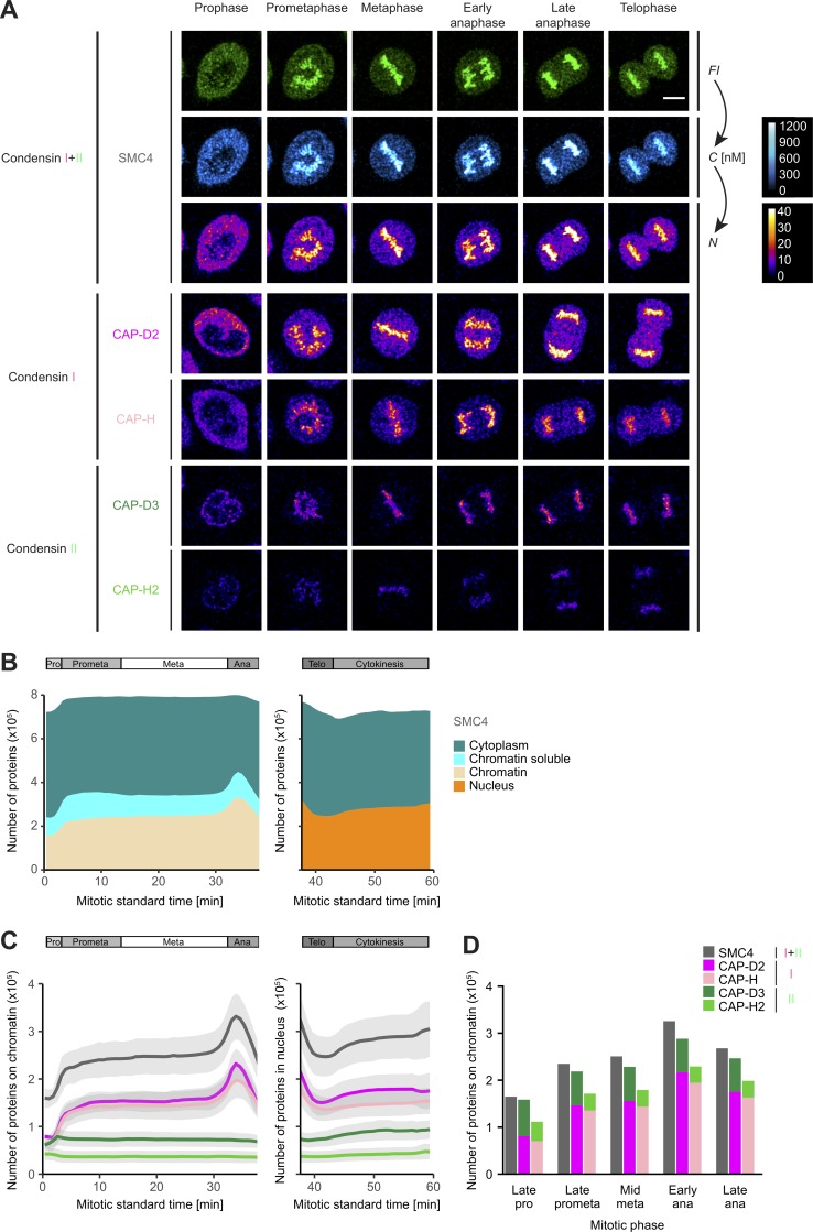
Figure 1.
Condensins I and II display different quantitative dynamics during mitosis as determined by automated FCS-calibrated confocal 3D time-lapse imaging. (A) Genome-edited HK cells with homozygously mEGFP-...
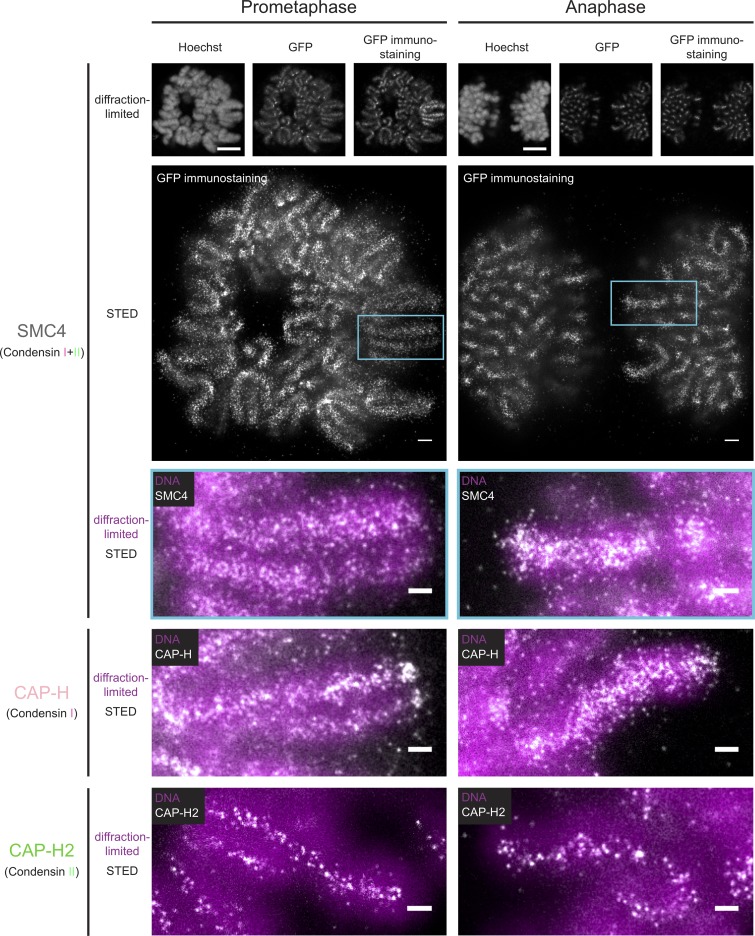
Figure 2.
STED superresolution imaging of Condensins I and II. Condensin subunits were immunostained (anti-GFP), and mitotic cells with chromatids oriented in parallel to the focal plane were selected for imagi...
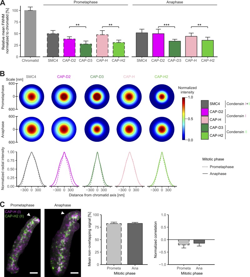
Figure 3.
Nonoverlapping localization of Condensins I and II along the mitotic chromatid axis. (A) The FWHM of Condensin subunit distribution and chromatid arms was analyzed (for details, see Fig. S3, A and B)....
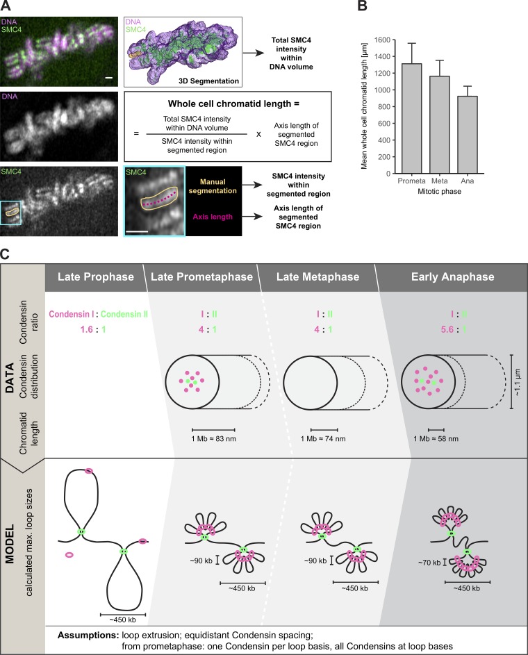
Figure 4.
A three-step hierarchical looping model of mitotic chromosome compaction based on a comprehensive 3D map of Condensins in human mitotic cells. (A and B) Whole chromatid length in mitotic HK cells. (A)...
Figure images are served from the NIH/NLM PubMed Central Open Access Subset or Europe PMC; copyright remains with the publishers and authors.
💬 Discussion
0 commentsNo comments yet. Be the first to start a discussion!
Leave a Comment