Abstract
Abstract DNA replication is a challenge for the faithful transmission of parental information to daughter cells, as both DNA and chromatin organization must be duplicated. Replication stress further complicates the safeguard of epigenome integrity. Here, we investigate the transmission of the histone variants H3.3 and H3.1 during replication. We follow their distribution relative to replication timing, first in the genome and, second, in 3D using super-resolution microscopy. We find that H3.3 and H3.1 mark early- and late-replicating chromatin, respectively. In the nucleus, H3.3 forms domains, which decrease in density throughout replication, while H3.1 domains increase in density. Hydroxyurea impairs local recycling of parental histones at replication sites. Similarly, depleting the histone chaperone ASF1 affects recycling, leading to an impaired histone variant landscape. We discuss how faithful transmission of histone variants involves ASF1 and can be impacted by replication stress, with ensuing consequences for cell fate and tumorigenesis.
🔬 Techniques
🔭 Microscopes
💻 Software
✨ Fluorophores
🧪 Sample Preparation
🔬 Cell Lines
🏭 Microscope Brands
🧪 Reagent Suppliers
📷 Detectors
🔎 Objectives
💻 Software Details
💾 Data Repositories
🏛️ Research Organizations (ROR)
Affiliated research institutions:
📋 Methods
H3.3- and H3.1-SNAP labeling in vivo We used cell lines stably expressing H3.3-SNAP-3xHA or H3.1-SNAP- 3xHA in HeLa cells previously used and characterized 12 . These cell lines have been tested negative for mycoplasma contamination. For the pulse experiments, we incubated cells in complete medium containing 2 μM of SNAP-Cell TMR-Star (New England Biolabs) and 10 μM of EdU during 20 min for labeling. We did two quick washes with phosphate-buffered saline (PBS) and then re-incubated the cells in complete medium for 30 min to allow excess SNAP-Cell TMR-Star to diffuse out. We then moved on to extraction and fixation protocol. For the pulse-chase experiments, we incubated cells with medium containing 2 μM of SNAP-Cell TMR-Star during 20 min for labeling, did two PBS washes and re-incubated the cells in complete medium for 30 min, and then washed twice with PBS again. We incubated the cells in complete medium for a chase period of 48 h. We then washed twice with PBS and re-incubated in complete medium containing 10 μM of EdU for 30 min, before moving on to extraction and fixation protocol. For the quench-chase-pulse experiments, we incubated cells in complete medium containing 10 μM of SNAP-Cell Block (New England Biolabs) to quench SNAP-tag activity, and then performed two PBS washes and 30 min of incubation in complete medium to allow the SNAP-Cell Block to diffuse out. We incubated in complete medium for a 2 h chase period, then performed a pulse step as described above. At least three independent experiments were performed for each condition.
Show full methods section
H3.3- and H3.1-SNAP labeling in vivo We used cell lines stably expressing H3.3-SNAP-3xHA or H3.1-SNAP- 3xHA in HeLa cells previously used and characterized 12 . These cell lines have been tested negative for mycoplasma contamination. For the pulse experiments, we incubated cells in complete medium containing 2 μM of SNAP-Cell TMR-Star (New England Biolabs) and 10 μM of EdU during 20 min for labeling. We did two quick washes with phosphate-buffered saline (PBS) and then re-incubated the cells in complete medium for 30 min to allow excess SNAP-Cell TMR-Star to diffuse out. We then moved on to extraction and fixation protocol. For the pulse-chase experiments, we incubated cells with medium containing 2 μM of SNAP-Cell TMR-Star during 20 min for labeling, did two PBS washes and re-incubated the cells in complete medium for 30 min, and then washed twice with PBS again. We incubated the cells in complete medium for a chase period of 48 h. We then washed twice with PBS and re-incubated in complete medium containing 10 μM of EdU for 30 min, before moving on to extraction and fixation protocol. For the quench-chase-pulse experiments, we incubated cells in complete medium containing 10 μM of SNAP-Cell Block (New England Biolabs) to quench SNAP-tag activity, and then performed two PBS washes and 30 min of incubation in complete medium to allow the SNAP-Cell Block to diffuse out. We incubated in complete medium for a 2 h chase period, then performed a pulse step as described above. At least three independent experiments were performed for each condition.
Extraction and fixation followed by EdU detection
We performed a pre-extraction of cells prior to fixation for 5 min with 0.5% Triton in CSK buffer (10 mM PIPES (pH 7), 100 mM NaCl, 300 mM sucrose, 3 mM MgCl 2 , protease inhibitors), then washed quickly with CSK and performed a 5 min CSK wash. We then fixed cells in 2% paraformaldehyde for 20 min. We blocked cells with bovine serum albumin (BSA; 3% in PBS) before performing Click reaction to reveal the EdU (Click-iT EdU Alexa Fluor 647 imaging kit, Invitrogen). We mounted the coverslips in PBS containing 5 mM of MEA (Mercaptoethylamine, 30070, Sigma) on cavity slides (BR475505, Sigma) and sealed with Twinsil sealing medium (Rotec) before STORM imaging. We changed the mounting buffer between every acquisition. siRNA transfection and drug treatment In the pulse-chase experiments, we performed a siRNA transfection prior to the pulse chase using Lipofectamine RNAimax (Invitrogen). We used siRNA previously characterized 30 , 31 against ASF1a (GUGAAGAAUACGAUCAAGUUU) and ASF1b (CAACGAGUACCUCAACCCUUU) at 100 nM concentration (siRNA purchased from Dharmacon). In hydroxyurea experiments, cells were treated with 3 mM HU for 30 min prior to extraction and fixation protocol.
Micrococcal nuclease sensitivity assay
One million cells of each indicated condition were collected, washed twice in PBS and nuclei were extracted in 150 mM NaCl, 50 mM Tris-HCl pH 7.5, 2 mM MgCl 2 , 0.1% Triton and 0.5% NP-40. Pelleted nuclei were re-suspended in 150 mM NaCl, 50 mM Tris-HCl pH 7.5, 2 mM MgCl 2 , 0.1% Triton and 5 mM CaCl 2 buffer, containing 2 units of S7 Micrococcal Nuclease (ThermoFisher Scientific EN0181) and incubated at 37 °C. At each time point, 20% of the sample was collected and mixed with an equal volume of 150 mM NaCl, 50 mM Tris-HCl pH 7.5, 2 mM MgCl 2 , 0.1% Triton and 10 mM EGTA to stop the digestion reaction. DNA was extracted, analyzed by electrophoresis in a 1% agarose gel with Sybr Safe dye (Invitrogen) and photographed under ultraviolet light using a ChemiDoc Gel Imaging System (Bio Rad). Images were analyzed with Fiji software to extract density profiles.
STORM imaging
We acquired 3D STORM images on a custom setup based on a Nikon iSPT-PALM inverted microscope. We excited Alexa 647—used to label EdU—with a 640 nm laser with a power of 10.8 mW at the sample. We excited TMR—used to label histones—with a 560 nm laser with a power of 41.3 mW at the sample. In addition, both for Alexa 647 and TMR, we used a 405 nm Coherent laser with a power of 18.5 μW at the sample. We imaged the fluorescence from the activated Alexa 647 and TMR molecules with an EM-CCD camera (Ixon Ultra 897 Andor) using a 100×/1.45NA (Nikon) objective. Using this objective, the image pixel size was 160 nm. We used a cylindrical lens (Melles Griot) for 3D 72 . We controlled the microscope with NIS software (Nikon). The number of acquisitions for each experiment is indicated in the figure legends. We detected the localizations in STORM movies with a custom algorithm as in Sergé et al. 73 . For data visualization, detections were rendered using the ViSP software as an isotropic Gaussian whose full-width half-maximum was 40 nm 74 . We performed z stacks on fluorescent beads (TetraSpeck Microspheres, ThermoFisher) for z calibration. We also used fluorescent beads monitored during STORM image acquisition to correct for sample drift 75 and to align the two signals. When two localizations were detected in consecutive frames within a 50 nm radius, we considered them as one.
STORM data analysis
We identified conglomerates of H3.3 and H3.1 or replication foci using the density-based clustering algorithm DBSCAN 76 . DBSCAN uses two input parameters—Eps and MinPts—and determines that a point is in a cluster if at least MinPts points are within a distance of Eps. We used an Eps value of 75 nm and a Minpts of 10 for DBSCAN analysis. For replication foci, we only used clusters with a detection number above a threshold value (100) for further analysis. To measure the volume of the conglomerates, we used the convex hull function in Matlab. For the density, we calculated the number of detections—normalized by the total number of detections in the nucleus—divided by the volume. We visualized the volume and density as distribution plots using the ksdensity function in Matlab. When looking at H3.3 or H3.1 conglomerates at replication sites, we selected the ones located under 200 nm from the center of gravity of an EdU cluster; we also tested selecting conglomerates directly situated in an EdU cluster using the convex hull function, which yielded the same results. To study parental H3.3 or H3.1 at replication sites, we calculated the number of H3.3 or H3.1 detections located in the replication foci—normalized by the total number of H3.3 or H3.1 detections in the nucleus—and normalized to the EdU signal, accounting for differences in replicative behavior, including between the two cell lines. This was also visualized as a distribution plot using ksdensity. When comparing populations, we used Mann Whitney Wilcoxon test. For comparison between scatter plots, error bars represent standard deviation and we used t -test. For the p values: p > 0.05 was annotated “ns” (non significant); *0.01 < p < 0.05; **0.001 < p < 0.01; and ***p < 0.001. For the study of spatial distribution, for each replication site, we assigned each surrounding detection of histones (for “histones vs EdU”)/EdU (for “EdU vs EdU”) to a 50 nm wide concentric region around the center of gravity of the replication site based on its distance to the center of gravity. The number of detections counted in each region was normalized by the volume of the corresponding region and plotted in a bar plot. For the alternative method, we modified the m function from Lang et al. 55 . We considered the distances between all the histone detections vs all the EdU detections and normalized to the distances between detections from two randomly distributed signals. In the plotted graph, when the function is above 1, it indicates attraction, while below 1 indicates repulsion.
Immunofluorescence and epifluorescence microscopy
For standard epifluorescence imaging of histone post-translational modifications, after blocking with BSA and Click reaction for EdU labeling, coverslips were incubated with primary and secondary antibodies and stained with DAPI. Coverslips were mounted in Vectashield medium. We used an AxioImager Zeiss Z1 microscope with a 63× objective. For confocal images, we used a Confocal Zeiss LSM780, and images were acquired using 63×/1.4NA under Zen blue software (Zeiss Germany). Antibodies were used at the following dilutions: H3K9me3 1:1000 (39765, ActiveMotif), H3K27me3 1:500 (07-449, Millipore), H3K4me3 1:500 (07-473, Millipore), H3K36me3 1:500 (ab9050, Abcam) and γH2AX 1:1000 (05-636, Euromedex).
H3.3 and H3.1 ChIP and ChIP-seq data analysis
We performed HA-tag ChIP-seq from the HeLa H3.3-SNAP-3xHA and HeLa H3.1-SNAP-3xHA cell lines as described in Rotem et al. 77 . We used 4 million cells digested in 100 μL with MNase for 8 min at 37 °C (3 units/million cell). We performed HA-ChIP by incubating chromatin (100 μL) supplemented with 500 μL incubation buffer (Tris-HCl 50 mM pH 7.5, NaCl 100 mM, BSA 0.5%, protease inhibitors tablet cocktail, Roche) with anti-HA beads (10 μL) (Roche diagnostics). After overnight incubation on a rotating wheel at 4 °C and following washes, we collected beads in 20 μL TE. We eliminated RNA contaminant by adding 2 μL RNAse A (10 μg/μL) and incubating 30 min at 37 °C. We eluted DNA by adding 2 μL Proteinase K (20 μg/μL), 2.5 μL SDS 2% and incubating 2 h at 37 °C. DNA was then purified with Agencourt AMPure XP Beads (Beckman Coulter) according to the manufacturer's recommendations in 20 μL water. Sequencing libraries (TruSeq ChIP) were prepared with 15 ng of DNA and paired-end sequenced on Illumina HiSeq 2500 at the Institut Curie Next Generation Sequencing (NGS) platform. Reads were aligned to the human genome version hg19/GRCh37 with Bowtie2 78 (version 2.2.9), run in paired-end mode using the very-sensitive parameter. Genome-wide coverage in bedGraph format was obtained for each alignment using bedtools 79 (version 2.17.0) after sorting and indexing the corresponding BAM file with samtools 80 (version 1.1). Custom Python scripts were used to compute the mean per-base coverage at consecutive 10 kb bins along each chromosome, after normalizing the read counts to the total sequencing depth for each sample. The log 2 ratio to input at non-zero bins was used as a proxy for H3 enrichment.
Data availability
All relevant data and analysis code for genome-wide and imaging experiments are available from the authors upon request. Raw sequencing data are available at the European Nucleotide Archive (ENA) under accession number PRJEB27519.
Electronic supplementary material Supplementary Information Peer Review File
Electronic supplementary material Supplementary Information accompanies this paper at 10.1038/s41467-018-05697-1.
📊 Figures
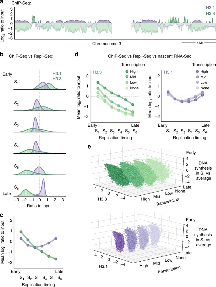
Fig. 1
Global H3.3 and H3.1 genome-wide occupancy relative to replication timing and transcriptional activity. a H3.3 and H3.1 genomic coverage normalized to input (chromosome 3 centromeric bandu00b115u2009M...
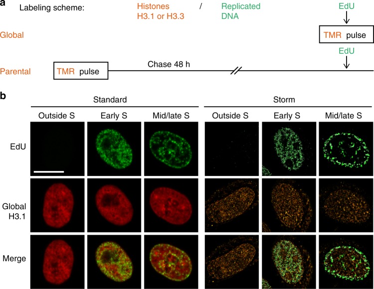
Fig. 2
Tracking histone H3 variants with STORM microscopy. a Labeling scheme using H3.3- or H3.1-SNAP to follow global (top) or parental (bottom) histones. A pulse using the fluorophore TMR (orange) labels S...
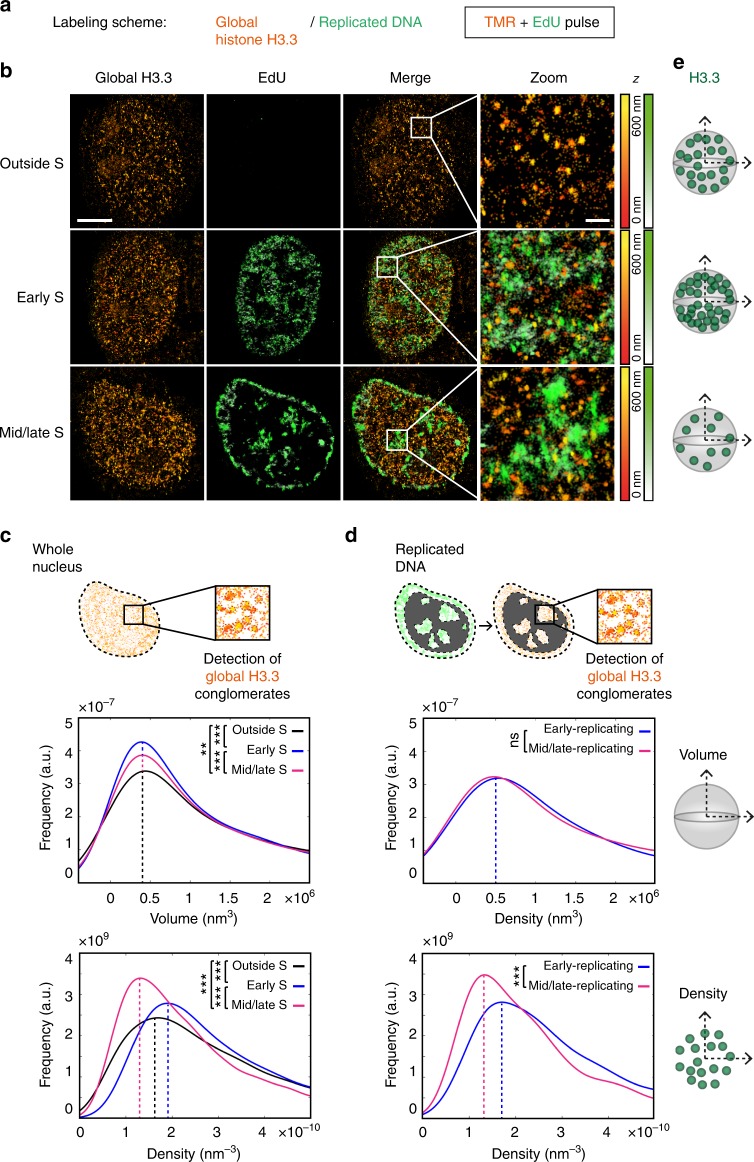
Fig. 3
Global distribution of H3.3 throughout S phase using STORM assay. a Labeling scheme using H3.3-SNAP to follow global H3.3 as described in Fig. 2 . b Representative STORM images of global H3.3 (TMR, or...
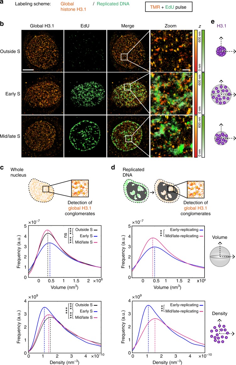
Fig. 4
Global distribution of H3.1 throughout S phase using STORM assay. a Labeling scheme using H3.1-SNAP to follow global H3.1 as described in Fig. 2 . b Representative STORM images of global H3.1 (TMR, or...
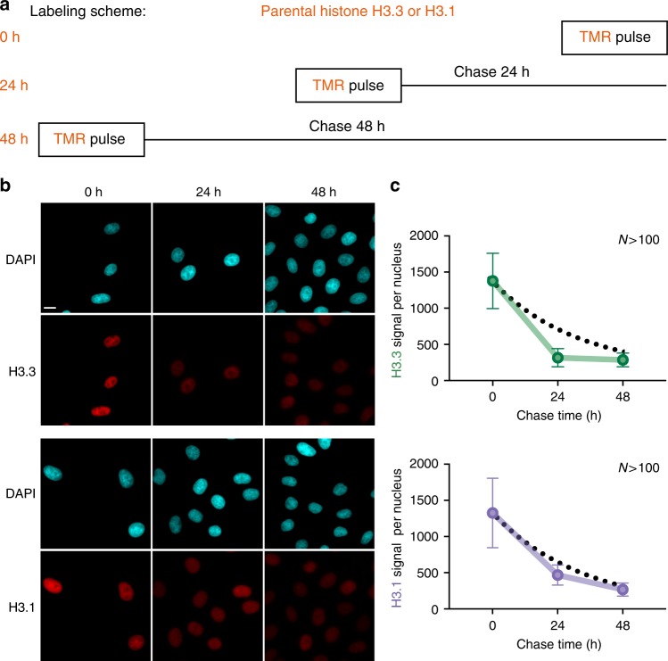
Fig. 5
Tracking parental H3.3 and H3.1 a Labeling scheme using H3.3- or H3.1-SNAP to follow parental H3.3 or H3.1 as described in Fig. 2 . We used three different chase times: 0, 24 and 48u2009h (equivalent ...
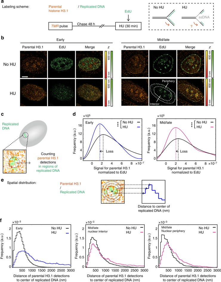
Fig. 6
Effect of hydroxyurea treatment on parental H3.1 recycling at replication sites. a Labeling scheme using H3.1-SNAP to follow parental H3.1 as described in Fig. 2 . In addition, we perform a 30u2009min...
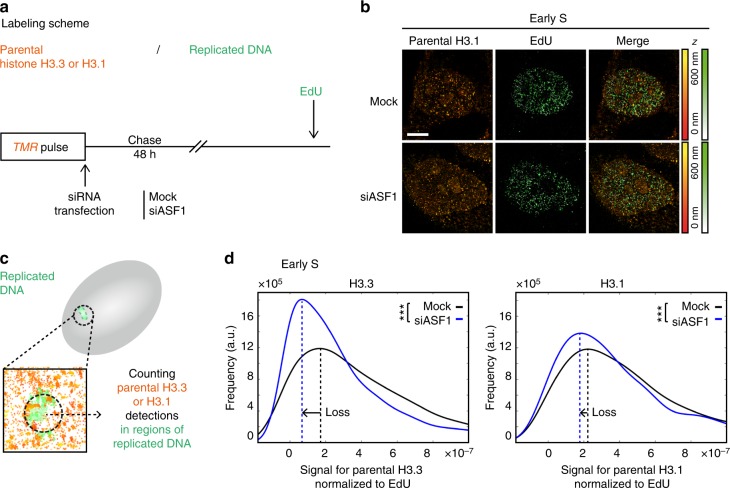
Fig. 7
Effect of ASF1 depletion on the recycling of parental H3.3 and H3.1 at replicated DNA regions. a Labeling scheme using H3.3- or H3.1-SNAP to follow parental H3.3 or H3.1 as described in Fig. 2 . In ad...
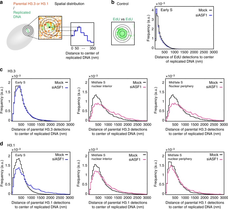
Fig. 8
Effect of ASF1 depletion on the spatial distribution of parental H3.3 and H3.1 throughout S phase. a Analysis method for the spatial distribution of parental H3.3 and H3.1 relative to replicated DNA a...
Figure images are served from the NIH/NLM PubMed Central Open Access Subset or Europe PMC; copyright remains with the publishers and authors.
💬 Discussion
0 commentsNo comments yet. Be the first to start a discussion!
Leave a Comment