Abstract
AbstractSingle-molecule localization microscopy (SMLM) can be used to resolve subcellular structures and achieve a tenfold improvement in spatial resolution compared to that obtained by conventional fluorescence microscopy. However, the separation of single-molecule fluorescence events that requires thousands of frames dramatically increases the image acquisition time and phototoxicity, impeding the observation of instantaneous intracellular dynamics. Here we develop a deep-learning based single-frame super-resolution microscopy (SFSRM) method which utilizes a subpixel edge map and a multicomponent optimization strategy to guide the neural network to reconstruct a super-resolution image from a single frame of a diffraction-limited image. Under a tolerable signal density and an affordable signal-to-noise ratio, SFSRM enables high-fidelity live-cell imaging with spatiotemporal resolutions of 30 nm and 10 ms, allowing for prolonged monitoring of subcellular dynamics such as interplays between mitochondria and endoplasmic reticulum, the vesicle transport along microtubules, and the endosome fusion and fission. Moreover, its adaptability to different microscopes and spectra makes it a useful tool for various imaging systems.
🔬 Techniques
🔭 Microscopes
✨ Fluorophores
🧪 Sample Preparation
🏭 Microscope Brands
🧪 Reagent Suppliers
📷 Detectors
🔎 Objectives
💻 Software Details
🏛️ Research Organizations (ROR)
Affiliated research institutions:
📋 Methods
SFSRM reconstructs a super-resolution image from a single experimental images of fixed cells We then tried to validate the resolution of SFSRM on experimental images. DNA origami nanorulers are standard samples that have two fluorescent markers with a specified mark-to-mark distance. To test SFSRM on DNA origami nanorulers, we first simulated dot pairs with an interpair distance ranging from 20 nm to 50 nm randomly distributed in GT images. The GT images were then blurred by a Gaussian kernel of a 280-nm FWHM size and followed by applying Poisson noise and Gaussian noise to get the LR images. The results in Supplementary Fig. 15 show that SFSRM accurately reconstructs 46%, 80%, 82%, and 84% dot pairs of 20-nm, 30-nm, 40-nm, and 50-nm interpair distances from the indistinguishable spots in the LR image, the reconstruction bias within half of the interpair distance is 76%, 99%, 99%, and 99% respectively, suggesting a reliable highest resolution at ~30 nm, similar to our observation on the simulated line pairs. We then used the trained SFSRM network to process the experimental WF images of DNA origami nanorulers with a 30-nm mark-to-mark distance (Fig. 2c ) . SFSRM clearly distinguished two spots and accurately reconstructed the distance between the two spots which is about 30 nm as measured from the STORM image. By contrast, a representative deep-learning-based super-resolution method called ANNA-PALM 31 is only able to reduce the size of the spot while failing to reconstruct the dot pairs from the blurred spots in the WF image given the challenging SNR of the WF image (e.g., SNR ~8). We then investigated the performance of SFSRM on the experimental images of subcellular structures. We first validated the effectiveness of the SFSRM method on experimental images of fixed microtubules. We collected training data (11 frames of STORM images with the corresponding WF images) of fixed microtubules stained with Alexa Fluor 647, and trained the network with different strategies. The results in Supplementary Fig. 16 suggest our approach can effectively improve the reconstruction resolution and reconstruction fidelity of fine structure compared to the basic ESRGAN generator trained with the pixel-wise loss (MS-SSIM-L1 loss). To test network robustness to different levels of experimental noise. A sequence of images of different SNRs was obtained and processed by the network. The reconstructed SR images were then compared with the corresponding STORM image by HAWKMAN analysis. The confidence maps indicate that the reconstruction errors increase as the SNR decreases (Supplementary Fig. 17 , LSNR-SR confidence map). When only SRN is used, the HAWKMAN score falls below 0.8 for SNR < 15, indicating a less reliable reconstruction result (Supplementary Fig. 17b , LSNR-SR). By contrast, if SEN is used in combination with SRN, the input SNR limit can be extended to SNR > 7 (Supplementary Fig. 17b , HSNR-SR). We compared the performance of SFSRM and ANNA-PALM on experimental images of microtubules in Fig. 2d . Although ANNA-PALM successfully reconstructs isolated microtubules, some of the microtubules are merged or lost in the reconstruction results where the microtubules are densely distributed (Fig. 2d , indicated by white arrows). In contrast, SFSRM correctly reconstructed most microtubules without losing or merging them even when they are close to each other. Quantitative assessment of the network reconstruction fidelity via HAWKMAN analysis demonstrates notably reduced local errors in the SFSRM reconstruction and on-average higher fidelity of the SFSRM reconstruction (HAWKMAN score: 0.95 vs. 0.90) (Fig. 2d , confidence maps). As depicted by the intensity profiles for the lines in Fig. 2d , two microtubules only 75 nm apart are indistinguishable in the ANNA-PALM reconstruction and are resolved in the SFSRM reconstruction result (Fig. 2d , plot), demonstrating a superior fine-structure reconstruction capability of SFSRM. In addition to our experimental data, SFSRM also achieves comparable reconstruction results to those via Deep-STORM 30 on the public dataset from the EPFL SMLM challenge website 39 (Supplementary Fig. 18 ). Unlike Deep-STORM which requires 300 frames of densely-distributed single-molecule images to reconstruct an SR image, SFSRM restores the SR image only from a single WF image, greatly reducing the photobleaching to the specimen as well as the data acquisition time. Apart from filaments, the performance of SFSRM on diverse subcellular structures is also promising. As shown in Fig. 2e , SFSRM resolves the ring-shaped clathrin-coated pits (CCPs) with diameters ranging from 50 nm to 160 nm from the noisy WF image. The estimated diameters of the CCPs from the SFSRM reconstructions show good consistency with that measured from the STORM images (Supplementary Fig. 19 ). We further benchmarked the performance of SFSRM on more subcellular structures including mitochondrial outer membrane, endoplasmic reticulum (ER), epidermal growth factor receptor (EGFR) protein, and nuclear pore complex proteins post a 2.5-fold expansion (Fig. 3a ). The reconstruction fidelity is measured by the MS-SSIM index of the SR images with respect to the STORM images, and the resolution is measured by decorrelation analysis 40 . SFSRM achieves in general an MS-SSIM score over 0.8 (Fig. 3b ) and resolutions of different structures ranging from 15 nm to 40 nm, consistent with those obtained from the corresponding STORM images (Fig. 3c ). In addition to the SR reconstruction of diverse organelles, SFSRM also demonstrates remarkable robustness to changes in imaging conditions including different imaging systems (Fig. 3d ) and different spectra (Fig. 3e ). Therefore, it serves as a versatile tool to transform different types of LR images to their SR counterparts by overcoming the limitations of SR microscopy such as requiring fluorophore blinking, long acquisition time, and high illuminance. Fig. 3 SFSRM applies to different subcellular structures, imaging systems, and spectra. a First row: representative WF images of mitochondria labeled with the mitochondrial membrane, endoplasmic reticulum (ER), EGFR protein after the EGF endocytosis, clathrin-coated pits after the EGF endocytosis, and expanded nuclear pore complex protein Nup133 (The specimen was expanded for 2.5 times with expansion microscopy after immunostaining). Second row: STORM images. Third row: corresponding SR images inferred from the WF images by SFSRM. b The reconstruction fidelity of SFSRM on different cellular structures measured by multi-scale structure similarity (MS-SSIM) index between the SFSRM and the corresponding STORM images. c The comparison of resolution (measured by decorrelation analysis) of SFSRM and the corresponding STORM images on different cellular structures. The error bars in b and c represent reconstruction experiments repeated on 25 images. All boxplots are drawn from the 25th to 75th percentile with the horizontal bar at the median and the whiskers extending to the minima and maxima. d The reconstruction results of WF images obtained from different imaging systems via SFSRM. The first column shows raw images obtained from a Zeiss Elyra 7 and the Zeiss sp8 confocal microscopes. Both WF images are processed by the SFSRM network to get the SR images in the second column. The SR images are compared with the STORM images and the differences are marked in the corresponding confidence maps in the third column. e The reconstruction results of WF images of microtubules separately labeled by dyes of different spectra. First column: WF images acquired from microtubules immunostained by Alexa Fluor 488, 568, and 647 separately. Second column: STORM images. Third column: SR images restored by the SFSRM network trained with images of microtubules stained by Alexa Fluor 647. Fourth column: confidence maps indicate the reconstruction errors in each SR image. The reconstruction results of the 488 and 568 channels have slightly lower HAWKMAN scores compared to that of the 647 channels, which might be caused by the inferior qualities of STORM images in the two channels. Scale bar, 2 µm ( a , d , e ), 1 µm (zoom-in view in a , d , e ).
Show full methods section
SFSRM reconstructs a super-resolution image from a single experimental images of fixed cells We then tried to validate the resolution of SFSRM on experimental images. DNA origami nanorulers are standard samples that have two fluorescent markers with a specified mark-to-mark distance. To test SFSRM on DNA origami nanorulers, we first simulated dot pairs with an interpair distance ranging from 20 nm to 50 nm randomly distributed in GT images. The GT images were then blurred by a Gaussian kernel of a 280-nm FWHM size and followed by applying Poisson noise and Gaussian noise to get the LR images. The results in Supplementary Fig. 15 show that SFSRM accurately reconstructs 46%, 80%, 82%, and 84% dot pairs of 20-nm, 30-nm, 40-nm, and 50-nm interpair distances from the indistinguishable spots in the LR image, the reconstruction bias within half of the interpair distance is 76%, 99%, 99%, and 99% respectively, suggesting a reliable highest resolution at ~30 nm, similar to our observation on the simulated line pairs. We then used the trained SFSRM network to process the experimental WF images of DNA origami nanorulers with a 30-nm mark-to-mark distance (Fig. 2c ) . SFSRM clearly distinguished two spots and accurately reconstructed the distance between the two spots which is about 30 nm as measured from the STORM image. By contrast, a representative deep-learning-based super-resolution method called ANNA-PALM 31 is only able to reduce the size of the spot while failing to reconstruct the dot pairs from the blurred spots in the WF image given the challenging SNR of the WF image (e.g., SNR ~8). We then investigated the performance of SFSRM on the experimental images of subcellular structures. We first validated the effectiveness of the SFSRM method on experimental images of fixed microtubules. We collected training data (11 frames of STORM images with the corresponding WF images) of fixed microtubules stained with Alexa Fluor 647, and trained the network with different strategies. The results in Supplementary Fig. 16 suggest our approach can effectively improve the reconstruction resolution and reconstruction fidelity of fine structure compared to the basic ESRGAN generator trained with the pixel-wise loss (MS-SSIM-L1 loss). To test network robustness to different levels of experimental noise. A sequence of images of different SNRs was obtained and processed by the network. The reconstructed SR images were then compared with the corresponding STORM image by HAWKMAN analysis. The confidence maps indicate that the reconstruction errors increase as the SNR decreases (Supplementary Fig. 17 , LSNR-SR confidence map). When only SRN is used, the HAWKMAN score falls below 0.8 for SNR < 15, indicating a less reliable reconstruction result (Supplementary Fig. 17b , LSNR-SR). By contrast, if SEN is used in combination with SRN, the input SNR limit can be extended to SNR > 7 (Supplementary Fig. 17b , HSNR-SR). We compared the performance of SFSRM and ANNA-PALM on experimental images of microtubules in Fig. 2d . Although ANNA-PALM successfully reconstructs isolated microtubules, some of the microtubules are merged or lost in the reconstruction results where the microtubules are densely distributed (Fig. 2d , indicated by white arrows). In contrast, SFSRM correctly reconstructed most microtubules without losing or merging them even when they are close to each other. Quantitative assessment of the network reconstruction fidelity via HAWKMAN analysis demonstrates notably reduced local errors in the SFSRM reconstruction and on-average higher fidelity of the SFSRM reconstruction (HAWKMAN score: 0.95 vs. 0.90) (Fig. 2d , confidence maps). As depicted by the intensity profiles for the lines in Fig. 2d , two microtubules only 75 nm apart are indistinguishable in the ANNA-PALM reconstruction and are resolved in the SFSRM reconstruction result (Fig. 2d , plot), demonstrating a superior fine-structure reconstruction capability of SFSRM. In addition to our experimental data, SFSRM also achieves comparable reconstruction results to those via Deep-STORM 30 on the public dataset from the EPFL SMLM challenge website 39 (Supplementary Fig. 18 ). Unlike Deep-STORM which requires 300 frames of densely-distributed single-molecule images to reconstruct an SR image, SFSRM restores the SR image only from a single WF image, greatly reducing the photobleaching to the specimen as well as the data acquisition time. Apart from filaments, the performance of SFSRM on diverse subcellular structures is also promising. As shown in Fig. 2e , SFSRM resolves the ring-shaped clathrin-coated pits (CCPs) with diameters ranging from 50 nm to 160 nm from the noisy WF image. The estimated diameters of the CCPs from the SFSRM reconstructions show good consistency with that measured from the STORM images (Supplementary Fig. 19 ). We further benchmarked the performance of SFSRM on more subcellular structures including mitochondrial outer membrane, endoplasmic reticulum (ER), epidermal growth factor receptor (EGFR) protein, and nuclear pore complex proteins post a 2.5-fold expansion (Fig. 3a ). The reconstruction fidelity is measured by the MS-SSIM index of the SR images with respect to the STORM images, and the resolution is measured by decorrelation analysis 40 . SFSRM achieves in general an MS-SSIM score over 0.8 (Fig. 3b ) and resolutions of different structures ranging from 15 nm to 40 nm, consistent with those obtained from the corresponding STORM images (Fig. 3c ). In addition to the SR reconstruction of diverse organelles, SFSRM also demonstrates remarkable robustness to changes in imaging conditions including different imaging systems (Fig. 3d ) and different spectra (Fig. 3e ). Therefore, it serves as a versatile tool to transform different types of LR images to their SR counterparts by overcoming the limitations of SR microscopy such as requiring fluorophore blinking, long acquisition time, and high illuminance. Fig. 3 SFSRM applies to different subcellular structures, imaging systems, and spectra. a First row: representative WF images of mitochondria labeled with the mitochondrial membrane, endoplasmic reticulum (ER), EGFR protein after the EGF endocytosis, clathrin-coated pits after the EGF endocytosis, and expanded nuclear pore complex protein Nup133 (The specimen was expanded for 2.5 times with expansion microscopy after immunostaining). Second row: STORM images. Third row: corresponding SR images inferred from the WF images by SFSRM. b The reconstruction fidelity of SFSRM on different cellular structures measured by multi-scale structure similarity (MS-SSIM) index between the SFSRM and the corresponding STORM images. c The comparison of resolution (measured by decorrelation analysis) of SFSRM and the corresponding STORM images on different cellular structures. The error bars in b and c represent reconstruction experiments repeated on 25 images. All boxplots are drawn from the 25th to 75th percentile with the horizontal bar at the median and the whiskers extending to the minima and maxima. d The reconstruction results of WF images obtained from different imaging systems via SFSRM. The first column shows raw images obtained from a Zeiss Elyra 7 and the Zeiss sp8 confocal microscopes. Both WF images are processed by the SFSRM network to get the SR images in the second column. The SR images are compared with the STORM images and the differences are marked in the corresponding confidence maps in the third column. e The reconstruction results of WF images of microtubules separately labeled by dyes of different spectra. First column: WF images acquired from microtubules immunostained by Alexa Fluor 488, 568, and 647 separately. Second column: STORM images. Third column: SR images restored by the SFSRM network trained with images of microtubules stained by Alexa Fluor 647. Fourth column: confidence maps indicate the reconstruction errors in each SR image. The reconstruction results of the 488 and 568 channels have slightly lower HAWKMAN scores compared to that of the 647 channels, which might be caused by the inferior qualities of STORM images in the two channels. Scale bar, 2 µm ( a , d , e ), 1 µm (zoom-in view in a , d , e ).
Methods SFSRM network Network architecture
The networks of our SFSRM, including the SEN and SRN, are based on the ESRGAN generator 25 , which includes 23 residual-in-residual dense blocks used to map low-resolution images to super-resolution images. By inheriting the basic architecture of SRGAN 24 , this network performs most computations in the LR feature space, hence reducing complexity and achieving high stability without requiring batch normalization (BN) layers 25 . The original ESRGAN is designed for a single RGB image. When it was applied to a grayscale image, we found that the network will easily crash at the beginning of or during the training process if we duplicate the grayscale image three times to generate a fake RGB input. Therefore, we adopted a single-channel ESRGAN generator. To incorporate the prior information provided by the edge map, we added another input channel to the network. The input LR image and the corresponding edge map are initially concatenated to generate a two-channel input to the generator. Similarly, duplicated grayscale images are used as fake RGB inputs to the well-trained VGG network 62 for feature map extraction. Loss functions To generate high-resolution details while maintaining high fidelity, the network is trained with a multicomponent loss function, as follows: Content loss evaluates the L 1 -norm distance between an estimated SR image documentclass[12pt]{minimal} usepackage{amsmath} usepackage{wasysym} usepackage{amsfonts} usepackage{amssymb} usepackage{amsbsy} usepackage{mathrsfs} usepackage{upgreek} setlength{oddsidemargin}{-69pt} begin{document}$${{{{{rm{G}}}}}}left(xright)$$end{document} G x and a GT image documentclass[12pt]{minimal} usepackage{amsmath} usepackage{wasysym} usepackage{amsfonts} usepackage{amssymb} usepackage{amsbsy} usepackage{mathrsfs} usepackage{upgreek} setlength{oddsidemargin}{-69pt} begin{document}$$y$$end{document} y . L 1 -norm loss focuses on pixel differences, thus allowing the network to quickly converge but often resulting in a blurred image. 1 documentclass[12pt]{minimal} usepackage{amsmath} usepackage{wasysym} usepackage{amsfonts} usepackage{amssymb} usepackage{amsbsy} usepackage{mathrsfs} usepackage{upgreek} setlength{oddsidemargin}{-69pt} begin{document}$${L}_{1}={{{{{rm{||G}}}}}}left(xright)-y{{{{{rm{||}}}}}}$$end{document} L 1 = ∣∣G x − y ∣∣ MS-SSIM measures the structural similarity of SR and GT images based on luminance, contrast, and structure at different scales. The computation of MS-SSIM is detailed in the assessment metrics section. Here, we focus on the construction of the loss function. MS-SSIM loss is defined as: 2 documentclass[12pt]{minimal} usepackage{amsmath} usepackage{wasysym} usepackage{amsfonts} usepackage{amssymb} usepackage{amsbsy} usepackage{mathrsfs} usepackage{upgreek} setlength{oddsidemargin}{-69pt} begin{document}$${L}_{{{{{{rm{MS}}}}}}-{{{{{rm{SSIM}}}}}}}=1-{{{{{rm{MS}}}}}}-{{{{{rm{SSIM}}}}}}left({{{{{rm{G}}}}}}left(xright),yright)$$end{document} L MS − SSIM = 1 − MS − SSIM G x , y Content loss is a hybrid of MS-SSIM loss and L 1 -norm loss and is noted as MS-SSIM-L1 loss: 3 documentclass[12pt]{minimal} usepackage{amsmath} usepackage{wasysym} usepackage{amsfonts} usepackage{amssymb} usepackage{amsbsy} usepackage{mathrsfs} usepackage{upgreek} setlength{oddsidemargin}{-69pt} begin{document}$${L}_{{{{{{rm{MS}}}}}}-{{{{{rm{SSIM}}}}}}-{{{{{rm{L}}}}}}1}=alpha cdot {L}_{{{{{{rm{MS}}}}}}-{{{{{rm{SSIM}}}}}}}+(1-alpha )cdot {L}_{1}$$end{document} L MS − SSIM − L 1 = α ⋅ L MS − SSIM + ( 1 − α ) ⋅ L 1 where documentclass[12pt]{minimal} usepackage{amsmath} usepackage{wasysym} usepackage{amsfonts} usepackage{amssymb} usepackage{amsbsy} usepackage{mathrsfs} usepackage{upgreek} setlength{oddsidemargin}{-69pt} begin{document}$$alpha$$end{document} α is used to balance the contributions of MS-SSIM loss and documentclass[12pt]{minimal} usepackage{amsmath} usepackage{wasysym} usepackage{amsfonts} usepackage{amssymb} usepackage{amsbsy} usepackage{mathrsfs} usepackage{upgreek} setlength{oddsidemargin}{-69pt} begin{document}$${L}_{1}$$end{document} L 1 -norm loss and is empirically set as documentclass[12pt]{minimal} usepackage{amsmath} usepackage{wasysym} usepackage{amsfonts} usepackage{amssymb} usepackage{amsbsy} usepackage{mathrsfs} usepackage{upgreek} setlength{oddsidemargin}{-69pt} begin{document}$$alpha=0.84$$end{document} α = 0.84 63 . Perceptual loss documentclass[12pt]{minimal} usepackage{amsmath} usepackage{wasysym} usepackage{amsfonts} usepackage{amssymb} usepackage{amsbsy} usepackage{mathrsfs} usepackage{upgreek} setlength{oddsidemargin}{-69pt} begin{document}$${L}_{{{{{{rm{Percep}}}}}}}$$end{document} L Percep is used to measure feature distance differences in the estimated SR image and corresponding GT image. Features are extracted by a VGG network 62 pretrained for material recognition and that is good at texture extraction. 4 documentclass[12pt]{minimal} usepackage{amsmath} usepackage{wasysym} usepackage{amsfonts} usepackage{amssymb} usepackage{amsbsy} usepackage{mathrsfs} usepackage{upgreek} setlength{oddsidemargin}{-69pt} begin{document}$${L}_{{{{{{rm{Percep}}}}}}}={{{{{rm{||F}}}}}}left({{{{{rm{G}}}}}}(x)right)-{{{{{rm{F}}}}}}(y){{{{{rm{||}}}}}}$$end{document} L Percep = ∣∣F G ( x ) − F ( y ) ∣∣ where F represents the feature extraction network. Adversarial loss estimates the probability that the discriminator input documentclass[12pt]{minimal} usepackage{amsmath} usepackage{wasysym} usepackage{amsfonts} usepackage{amssymb} usepackage{amsbsy} usepackage{mathrsfs} usepackage{upgreek} setlength{oddsidemargin}{-69pt} begin{document}$$x$$end{document} x is real or fake. Here we use U-net as the discriminator, which has an encoder and a decoder. The discriminator is trained to provide both global and pixelwise decisions on whether the input image is real or fake 64 . Specifically, an input real image documentclass[12pt]{minimal} usepackage{amsmath} usepackage{wasysym} usepackage{amsfonts} usepackage{amssymb} usepackage{amsbsy} usepackage{mathrsfs} usepackage{upgreek} setlength{oddsidemargin}{-69pt} begin{document}$$y$$end{document} y or fake image documentclass[12pt]{minimal} usepackage{amsmath} usepackage{wasysym} usepackage{amsfonts} usepackage{amssymb} usepackage{amsbsy} usepackage{mathrsfs} usepackage{upgreek} setlength{oddsidemargin}{-69pt} begin{document}$${{{{{rm{G}}}}}}(x)$$end{document} G ( x ) will be first gradually convolved by the encoder to one pixel to get a global decision on whether this image is real or fake, then the input will be gradually deconvolved by the decoder to its original size to get a per-pixel decision on whether this pixel is real or fake. The encoder and decoder are trained by the following losses: 5 documentclass[12pt]{minimal} usepackage{amsmath} usepackage{wasysym} usepackage{amsfonts} usepackage{amssymb} usepackage{amsbsy} usepackage{mathrsfs} usepackage{upgreek} setlength{oddsidemargin}{-69pt} begin{document}$${L}_{{{{{rm{enc}}}}}}=-{{{{{rm{E}}}}}}left[{log }{D}_{{{{{rm{enc}}}}}}left( y right)right]-{{{{{rm{E}}}}}}left[{log }(1-{D}_{{{{{{rm{enc}}}}}}}left({{{{{rm{G}}}}}}(x)right))right]$$end{document} L enc = − E log D enc y − E log ( 1 − D enc G ( x ) ) 6 documentclass[12pt]{minimal} usepackage{amsmath} usepackage{wasysym} usepackage{amsfonts} usepackage{amssymb} usepackage{amsbsy} usepackage{mathrsfs} usepackage{upgreek} setlength{oddsidemargin}{-69pt} begin{document}$${L}_{{{{{{rm{dec}}}}}}}=-{{{{{rm{E}}}}}}left[mathop{sum}limits_{i,j}{log }{left[{D}_{{{{{{rm{dec}}}}}}}left(yright)right]}_{i,j}right]-{{{{{rm{E}}}}}}left[mathop{sum}limits_{i,j}{log }(1-{left[{D}_{{{{{{rm{dec}}}}}}}left({{{{{rm{G}}}}}}(x)right)right]}_{i,j})right]$$end{document} L dec = − E ∑ i , j log D dec y i , j − E ∑ i , j log ( 1 − D dec G ( x ) i , j ) where documentclass[12pt]{minimal} usepackage{amsmath} usepackage{wasysym} usepackage{amsfonts} usepackage{amssymb} usepackage{amsbsy} usepackage{mathrsfs} usepackage{upgreek} setlength{oddsidemargin}{-69pt} begin{document}$${D}_{{{{{{rm{enc}}}}}}}left( cdot right)$$end{document} D enc ⋅ is the encoder decision of the whole input and documentclass[12pt]{minimal} usepackage{amsmath} usepackage{wasysym} usepackage{amsfonts} usepackage{amssymb} usepackage{amsbsy} usepackage{mathrsfs} usepackage{upgreek} setlength{oddsidemargin}{-69pt} begin{document}$${left[{D}_{{{{{{rm{dec}}}}}}}left(cdotright)right]}_{i,j}$$end{document} D dec ⋅ i , j is the decoder decision at pixel documentclass[12pt]{minimal} usepackage{amsmath} usepackage{wasysym} usepackage{amsfonts} usepackage{amssymb} usepackage{amsbsy} usepackage{mathrsfs} usepackage{upgreek} setlength{oddsidemargin}{-69pt} begin{document}$$left(i,, jright)$$end{document} i , j ; E[·] represents taking the average for all data in the minibatch. The discriminator is trained by both encoder loss and decoder loss. 7 documentclass[12pt]{minimal} usepackage{amsmath} usepackage{wasysym} usepackage{amsfonts} usepackage{amssymb} usepackage{amsbsy} usepackage{mathrsfs} usepackage{upgreek} setlength{oddsidemargin}{-69pt} begin{document}$${L}_{D}={L}_{{{{{{rm{enc}}}}}}}+{L}_{{{{{{rm{dec}}}}}}}$$end{document} L D = L enc + L dec Correspondingly, the discriminator feedback to the generator, i.e., the adversarial loss is formulated as 8 documentclass[12pt]{minimal} usepackage{amsmath} usepackage{wasysym} usepackage{amsfonts} usepackage{amssymb} usepackage{amsbsy} usepackage{mathrsfs} usepackage{upgreek} setlength{oddsidemargin}{-69pt} begin{document}$${L}_{{{{{{rm{Adv}}}}}}}=-{{{{{rm{E}}}}}}[{log }{D}_{{{{{{rm{enc}}}}}}}left({{{{{rm{G}}}}}}(x)right)]-{{{{{rm{E}}}}}}left[mathop{sum}limits_{i,j}{log }{left[{D}_{{{{{{rm{dec}}}}}}}left({{{{{rm{G}}}}}}(x)right)right]}_{i,j}right]$$end{document} L Adv = − E [ log D enc G ( x ) ] − E ∑ i , j log D dec G ( x ) i , j Frequency loss compares the frequency difference between an estimated SR and the original GT image: 9 documentclass[12pt]{minimal} usepackage{amsmath} usepackage{wasysym} usepackage{amsfonts} usepackage{amssymb} usepackage{amsbsy} usepackage{mathrsfs} usepackage{upgreek} setlength{oddsidemargin}{-69pt} begin{document}$${L}_{{{{{{rm{Freq}}}}}}}={{{{{rm{||FFT}}}}}}left({{{{{rm{G}}}}}}(x)right)-{{{{{rm{FFT}}}}}}(y){{{{{rm{||}}}}}}$$end{document} L Freq = ∣∣FFT G ( x ) − FFT ( y ) ∣∣ where FFT is the fast Fourier transformation function. We compared all frequency components when the GT images do not contain noise and 75% of frequency components when the GT images contain noise, for experimental images as well as some simulation images. When using the ESRGAN as SEN for signal enhancement, the network only uses LR images as single-channel inputs. The training of the SEN includes two steps: Training with MS-SSIM-L1 loss for ~100,000 minibatch iterations at a 3 × 10 −4 learning rate 10 documentclass[12pt]{minimal} usepackage{amsmath} usepackage{wasysym} usepackage{amsfonts} usepackage{amssymb} usepackage{amsbsy} usepackage{mathrsfs} usepackage{upgreek} setlength{oddsidemargin}{-69pt} begin{document}$${L}_{{{{{{rm{G}}}}}}}={L}_{{{{{{rm{MS}}}}}}-{{{{{rm{SSIM}}}}}}-{{{{{rm{L}}}}}}1}$$end{document} L G = L MS − SSIM − L 1 Training with MS-SSIM-L1 loss and perceptual loss for 20,000 to 50,000 minibatch iterations at a 1 × 10 −4 learning rate. 11 documentclass[12pt]{minimal} usepackage{amsmath} usepackage{wasysym} usepackage{amsfonts} usepackage{amssymb} usepackage{amsbsy} usepackage{mathrsfs} usepackage{upgreek} setlength{oddsidemargin}{-69pt} begin{document}$${L}_{{{{{{rm{G}}}}}}}={L}_{{{{{{rm{MS}}}}}}-{{{{{rm{SSIM}}}}}}-{{{{{rm{L}}}}}}1}+{delta cdot L}_{{{{{{rm{percep}}}}}}}$$end{document} L G = L MS − SSIM − L 1 + δ ⋅ L percep where documentclass[12pt]{minimal} usepackage{amsmath} usepackage{wasysym} usepackage{amsfonts} usepackage{amssymb} usepackage{amsbsy} usepackage{mathrsfs} usepackage{upgreek} setlength{oddsidemargin}{-69pt} begin{document}$$delta$$end{document} δ is the coefficient to balance different loss components and we empirically set documentclass[12pt]{minimal} usepackage{amsmath} usepackage{wasysym} usepackage{amsfonts} usepackage{amssymb} usepackage{amsbsy} usepackage{mathrsfs} usepackage{upgreek} setlength{oddsidemargin}{-69pt} begin{document}$$delta=0.1$$end{document} δ = 0.1 . When using the ESRGAN as SRN for super-resolution restoration, the network uses both LR images and edge maps as inputs. The training process also includes two stages. The first stage uses the same loss function as the SEN, and the second stage uses the following loss function with a 5 × 10 −5 learning rate for ~10,000 minibatch iterations. 12 documentclass[12pt]{minimal} usepackage{amsmath} usepackage{wasysym} usepackage{amsfonts} usepackage{amssymb} usepackage{amsbsy} usepackage{mathrsfs} usepackage{upgreek} setlength{oddsidemargin}{-69pt} begin{document}$${L}_{G}={L}_{{{{{{rm{MS}}}}}}-{{{{{rm{SSIM}}}}}}-{{{{{rm{L}}}}}}1}+{delta cdot L}_{{{{{{rm{Percep}}}}}}}+beta cdot {L}_{{{{{{rm{Adv}}}}}}}+gamma cdot {L}_{{{{{{rm{Freq}}}}}}}$$end{document} L G = L MS − SSIM − L 1 + δ ⋅ L Percep + β ⋅ L Adv + γ ⋅ L Freq In our experiments, we empirically set documentclass[12pt]{minimal} usepackage{amsmath} usepackage{wasysym} usepackage{amsfonts} usepackage{amssymb} usepackage{amsbsy} usepackage{mathrsfs} usepackage{upgreek} setlength{oddsidemargin}{-69pt} begin{document}$$delta$$end{document} δ , documentclass[12pt]{minimal} usepackage{amsmath} usepackage{wasysym} usepackage{amsfonts} usepackage{amssymb} usepackage{amsbsy} usepackage{mathrsfs} usepackage{upgreek} setlength{oddsidemargin}{-69pt} begin{document}$$beta$$end{document} β , documentclass[12pt]{minimal} usepackage{amsmath} usepackage{wasysym} usepackage{amsfonts} usepackage{amssymb} usepackage{amsbsy} usepackage{mathrsfs} usepackage{upgreek} setlength{oddsidemargin}{-69pt} begin{document}$$gamma$$end{document} γ and to documentclass[12pt]{minimal} usepackage{amsmath} usepackage{wasysym} usepackage{amsfonts} usepackage{amssymb} usepackage{amsbsy} usepackage{mathrsfs} usepackage{upgreek} setlength{oddsidemargin}{-69pt} begin{document}$$delta=0.1$$end{document} δ = 0.1 , documentclass[12pt]{minimal} usepackage{amsmath} usepackage{wasysym} usepackage{amsfonts} usepackage{amssymb} usepackage{amsbsy} usepackage{mathrsfs} usepackage{upgreek} setlength{oddsidemargin}{-69pt} begin{document}$$beta=0.001$$end{document} β = 0.001 , and documentclass[12pt]{minimal} usepackage{amsmath} usepackage{wasysym} usepackage{amsfonts} usepackage{amssymb} usepackage{amsbsy} usepackage{mathrsfs} usepackage{upgreek} setlength{oddsidemargin}{-69pt} begin{document}$$gamma=0.01$$end{document} γ = 0.01 , respectively.
Assessment metrics
Multiscale structure similarity (MS-SSIM) 65 quantifies the similarity of two images and is an improvement of SSIM 66 , which assesses the similarity between two images, documentclass[12pt]{minimal} usepackage{amsmath} usepackage{wasysym} usepackage{amsfonts} usepackage{amssymb} usepackage{amsbsy} usepackage{mathrsfs} usepackage{upgreek} setlength{oddsidemargin}{-69pt} begin{document}$$x$$end{document} x and documentclass[12pt]{minimal} usepackage{amsmath} usepackage{wasysym} usepackage{amsfonts} usepackage{amssymb} usepackage{amsbsy} usepackage{mathrsfs} usepackage{upgreek} setlength{oddsidemargin}{-69pt} begin{document}$$y$$end{document} y , based on three factors: luminance documentclass[12pt]{minimal} usepackage{amsmath} usepackage{wasysym} usepackage{amsfonts} usepackage{amssymb} usepackage{amsbsy} usepackage{mathrsfs} usepackage{upgreek} setlength{oddsidemargin}{-69pt} begin{document}$$lleft(x,, yright)$$end{document} l x , y , contrast documentclass[12pt]{minimal} usepackage{amsmath} usepackage{wasysym} usepackage{amsfonts} usepackage{amssymb} usepackage{amsbsy} usepackage{mathrsfs} usepackage{upgreek} setlength{oddsidemargin}{-69pt} begin{document}$$cleft(x,, yright)$$end{document} c x , y , and structure documentclass[12pt]{minimal} usepackage{amsmath} usepackage{wasysym} usepackage{amsfonts} usepackage{amssymb} usepackage{amsbsy} usepackage{mathrsfs} usepackage{upgreek} setlength{oddsidemargin}{-69pt} begin{document}$$sleft(x,yright)$$end{document} s x , y . 13 documentclass[12pt]{minimal} usepackage{amsmath} usepackage{wasysym} usepackage{amsfonts} usepackage{amssymb} usepackage{amsbsy} usepackage{mathrsfs} usepackage{upgreek} setlength{oddsidemargin}{-69pt} begin{document}$$lleft(x,yright)=frac{2{u}_{{{{{{rm{x}}}}}}}{u}_{{{{{{rm{y}}}}}}}+{C}_{1}}{{{u}_{{{{{{rm{x}}}}}}}}^{2}{{u}_{{{{{{rm{y}}}}}}}}^{2}+{C}_{1}}$$end{document} l x , y = 2 u x u y + C 1 u x 2 u y 2 + C 1 14 documentclass[12pt]{minimal} usepackage{amsmath} usepackage{wasysym} usepackage{amsfonts} usepackage{amssymb} usepackage{amsbsy} usepackage{mathrsfs} usepackage{upgreek} setlength{oddsidemargin}{-69pt} begin{document}$$cleft(x,yright)=frac{2{sigma }_{{{{{{rm{x}}}}}}}{sigma }_{{{{{{rm{y}}}}}}}+{C}_{2}}{{{sigma }_{{{{{{rm{x}}}}}}}}^{2}{{sigma }_{{{{{{rm{y}}}}}}}}^{2}+{C}_{2}}$$end{document} c x , y = 2 σ x σ y + C 2 σ x 2 σ y 2 + C 2 15 documentclass[12pt]{minimal} usepackage{amsmath} usepackage{wasysym} usepackage{amsfonts} usepackage{amssymb} usepackage{amsbsy} usepackage{mathrsfs} usepackage{upgreek} setlength{oddsidemargin}{-69pt} begin{document}$$sleft(x,yright)=frac{2{sigma }_{{{{{{rm{xy}}}}}}}+{C}_{3}}{{sigma }_{{{{{{rm{x}}}}}}}{sigma }_{{{{{{rm{y}}}}}}}+{C}_{3}}$$end{document} s x , y = 2 σ xy + C 3 σ x σ y + C 3 where documentclass[12pt]{minimal} usepackage{amsmath} usepackage{wasysym} usepackage{amsfonts} usepackage{amssymb} usepackage{amsbsy} usepackage{mathrsfs} usepackage{upgreek} setlength{oddsidemargin}{-69pt} begin{document}$${u}_{{{{{{rm{x}}}}}}}{,, u}_{{{{{{rm{y}}}}}}}$$end{document} u x , u y represent the average of documentclass[12pt]{minimal} usepackage{amsmath} usepackage{wasysym} usepackage{amsfonts} usepackage{amssymb} usepackage{amsbsy} usepackage{mathrsfs} usepackage{upgreek} setlength{oddsidemargin}{-69pt} begin{document}$$x,, y$$end{document} x , y ; documentclass[12pt]{minimal} usepackage{amsmath} usepackage{wasysym} usepackage{amsfonts} usepackage{amssymb} usepackage{amsbsy} usepackage{mathrsfs} usepackage{upgreek} setlength{oddsidemargin}{-69pt} begin{document}$${sigma }_{{{{{{rm{x}}}}}}},, {sigma }_{{{{{{rm{y}}}}}}}$$end{document} σ x , σ y represent the variance of documentclass[12pt]{minimal} usepackage{amsmath} usepackage{wasysym} usepackage{amsfonts} usepackage{amssymb} usepackage{amsbsy} usepackage{mathrsfs} usepackage{upgreek} setlength{oddsidemargin}{-69pt} begin{document}$$x,y$$end{document} x , y ; documentclass[12pt]{minimal} usepackage{amsmath} usepackage{wasysym} usepackage{amsfonts} usepackage{amssymb} usepackage{amsbsy} usepackage{mathrsfs} usepackage{upgreek} setlength{oddsidemargin}{-69pt} begin{document}$${C}_{1}$$end{document} C 1 , documentclass[12pt]{minimal} usepackage{amsmath} usepackage{wasysym} usepackage{amsfonts} usepackage{amssymb} usepackage{amsbsy} usepackage{mathrsfs} usepackage{upgreek} setlength{oddsidemargin}{-69pt} begin{document}$${C}_{2}$$end{document} C 2 and documentclass[12pt]{minimal} usepackage{amsmath} usepackage{wasysym} usepackage{amsfonts} usepackage{amssymb} usepackage{amsbsy} usepackage{mathrsfs} usepackage{upgreek} setlength{oddsidemargin}{-69pt} begin{document}$${C}_{3}$$end{document} C 3 are small constants given by documentclass[12pt]{minimal} usepackage{amsmath} usepackage{wasysym} usepackage{amsfonts} usepackage{amssymb} usepackage{amsbsy} usepackage{mathrsfs} usepackage{upgreek} setlength{oddsidemargin}{-69pt} begin{document}$${C}_{1}={({K}_{1}L)}^{2}$$end{document} C 1 = ( K 1 L ) 2 , documentclass[12pt]{minimal} usepackage{amsmath} usepackage{wasysym} usepackage{amsfonts} usepackage{amssymb} usepackage{amsbsy} usepackage{mathrsfs} usepackage{upgreek} setlength{oddsidemargin}{-69pt} begin{document}$${C}_{2}={({K}_{2}L)}^{2}$$end{document} C 2 = ( K 2 L ) 2 , and documentclass[12pt]{minimal} usepackage{amsmath} usepackage{wasysym} usepackage{amsfonts} usepackage{amssymb} usepackage{amsbsy} usepackage{mathrsfs} usepackage{upgreek} setlength{oddsidemargin}{-69pt} begin{document}$${C}_{3}={C}_{2}/2$$end{document} C 3 = C 2 / 2 . Here documentclass[12pt]{minimal} usepackage{amsmath} usepackage{wasysym} usepackage{amsfonts} usepackage{amssymb} usepackage{amsbsy} usepackage{mathrsfs} usepackage{upgreek} setlength{oddsidemargin}{-69pt} begin{document}$$L$$end{document} L is the dynamic range of pixel values, and documentclass[12pt]{minimal} usepackage{amsmath} usepackage{wasysym} usepackage{amsfonts} usepackage{amssymb} usepackage{amsbsy} usepackage{mathrsfs} usepackage{upgreek} setlength{oddsidemargin}{-69pt} begin{document}$${K}_{1}$$end{document} K 1 and documentclass[12pt]{minimal} usepackage{amsmath} usepackage{wasysym} usepackage{amsfonts} usepackage{amssymb} usepackage{amsbsy} usepackage{mathrsfs} usepackage{upgreek} setlength{oddsidemargin}{-69pt} begin{document}$${K}_{2}$$end{document} K 2 are two scalar constants. The general form of SSIM is defined as: 16 documentclass[12pt]{minimal} usepackage{amsmath} usepackage{wasysym} usepackage{amsfonts} usepackage{amssymb} usepackage{amsbsy} usepackage{mathrsfs} usepackage{upgreek} setlength{oddsidemargin}{-69pt} begin{document}$${{{{{rm{SSIM}}}}}}left(x,, yright)={left[lleft(x,, yright)right]}^{alpha }{left[cleft(x,, yright)right]}^{beta }{left[sleft(x,, yright)right]}^{gamma }$$end{document} SSIM x , y = l x , y α c x , y β s x , y γ where documentclass[12pt]{minimal} usepackage{amsmath} usepackage{wasysym} usepackage{amsfonts} usepackage{amssymb} usepackage{amsbsy} usepackage{mathrsfs} usepackage{upgreek} setlength{oddsidemargin}{-69pt} begin{document}$$alpha$$end{document} α , documentclass[12pt]{minimal} usepackage{amsmath} usepackage{wasysym} usepackage{amsfonts} usepackage{amssymb} usepackage{amsbsy} usepackage{mathrsfs} usepackage{upgreek} setlength{oddsidemargin}{-69pt} begin{document}$$beta$$end{document} β , and documentclass[12pt]{minimal} usepackage{amsmath} usepackage{wasysym} usepackage{amsfonts} usepackage{amssymb} usepackage{amsbsy} usepackage{mathrsfs} usepackage{upgreek} setlength{oddsidemargin}{-69pt} begin{document}$$gamma$$end{document} γ are parameters used to define the relative importance of the three components and are set to 1 in most cases 66 . MS-SSIM is calculated by iteratively applying low-pass filters, down sampling the filtered image result by a factor M and then calculating the SSIM index of the scaled images. The overall MS-SSIM evaluation is based on combining the measurements at different scales: 17 documentclass[12pt]{minimal} usepackage{amsmath} usepackage{wasysym} usepackage{amsfonts} usepackage{amssymb} usepackage{amsbsy} usepackage{mathrsfs} usepackage{upgreek} setlength{oddsidemargin}{-69pt} begin{document}$${{{{{rm{MS}}}}}}-{{{{{rm{SSIM}}}}}}left(x,, yright)={left[lleft(x,, yright)right]}^{{alpha }_{{{{{{rm{j}}}}}}}M}.mathop{prod }limits_{j=1}^{M}{left[{c}_{{{{{{rm{j}}}}}}}left(x,, yright)right]}^{{beta }_{{{{{{rm{j}}}}}}}}{left[{s}_{{{{{{rm{j}}}}}}}left(x,, yright)right]}^{{gamma }_{{{{{{rm{j}}}}}}}}$$end{document} MS − SSIM x , y = l x , y α j M . ∏ j = 1 M c j x , y β j s j x , y γ j where documentclass[12pt]{minimal} usepackage{amsmath} usepackage{wasysym} usepackage{amsfonts} usepackage{amssymb} usepackage{amsbsy} usepackage{mathrsfs} usepackage{upgreek} setlength{oddsidemargin}{-69pt} begin{document}$${alpha }_{{{{{{rm{j}}}}}}}$$end{document} α j , documentclass[12pt]{minimal} usepackage{amsmath} usepackage{wasysym} usepackage{amsfonts} usepackage{amssymb} usepackage{amsbsy} usepackage{mathrsfs} usepackage{upgreek} setlength{oddsidemargin}{-69pt} begin{document}$${beta }_{{{{{{rm{j}}}}}}}$$end{document} β j , and documentclass[12pt]{minimal} usepackage{amsmath} usepackage{wasysym} usepackage{amsfonts} usepackage{amssymb} usepackage{amsbsy} usepackage{mathrsfs} usepackage{upgreek} setlength{oddsidemargin}{-69pt} begin{document}$${gamma }_{{{{{{rm{j}}}}}}}$$end{document} γ j are used to adjust the relative importance of different components 65 . HAWKMAN analysis 38 assesses the similarity of two images based on their structures rather than their intensity, making it suitable for SMLM images whose intensity is not linearly related to the labeling density. In HAWKMAN analysis, two images are first normalized and blurred by Gaussian kernels with successive sizes up to a user-specified maximum, and the blurred images are then normalized by the maximum intensity of one. Next, the images are binarised based on the local threshold to extract the feature signals. The obtained images are regarded as sharpening images. The sharpening images are further blurred and flattened, re-binarised at a higher threshold, and then skeletonized to get skeletonized images. The skeletonized images are re-blurred with a Gaussian kernel of FWHM equal to the original scale to get the structure images. Finally, the cross-correlations of the sharpening images and the structure images are calculated to yield a confidence score of the test image (here we note as HAWKMAN score). And a confidence map is produced and a local confidence score below 0.85 indicates that the structures are less trustable. 18 documentclass[12pt]{minimal} usepackage{amsmath} usepackage{wasysym} usepackage{amsfonts} usepackage{amssymb} usepackage{amsbsy} usepackage{mathrsfs} usepackage{upgreek} setlength{oddsidemargin}{-69pt} begin{document}$${{{{{rm{HAWKMAN}}}}}}; {{{{{rm{score}}}}}}=frac{1}{2}{min }left(1,frac{{{{{{{rm{PCC}}}}}}}^{{{{{{rm{sharp}}}}}}}}{0.85}right)+frac{1}{2}{min }left(1,frac{{{{{{{rm{PCC}}}}}}}^{{{{{{rm{str}}}}}}}}{0.85}right)$$end{document} HAWKMAN score = 1 2 min 1 , PCC sharp 0.85 + 1 2 min 1 , PCC str 0.85 where PCC sharp and PCC str are the Pearson correlation coefficients for the sharpening and structure images. Signal density is computed from a GT image by first conducting binarization for the image to extract the signal-containing pixels and then calculating the ratio of the number of signal-containing pixels to the total number of pixels in the image. 19 documentclass[12pt]{minimal} usepackage{amsmath} usepackage{wasysym} usepackage{amsfonts} usepackage{amssymb} usepackage{amsbsy} usepackage{mathrsfs} usepackage{upgreek} setlength{oddsidemargin}{-69pt} begin{document}$${{{{{rm{signal; density}}}}}}=frac{{{{{{{rm{Pixel}}}}}}}_{{{{{{rm{signal}}}}}}}}{{{{{{{rm{Pixel}}}}}}}_{{{{{{rm{total}}}}}}}}$$end{document} signal density = Pixel signal Pixel total Simulation image generation For the simulation of polymer lines, simulated polymer chains in a 10 × 10 µm 2 region were generated in MATLAB. The polymer density was set to 50 polymers per image to mimic a densely distributed microtubule network. The GT image was created by fitting the fluorophore positions to an image with a pixel size of 10 nm and convolved with a Gaussian kernel of a 20-nm FWHM size. For the GT image, no noise and a uniform background were used. Similar to the process of generating the GT image, the corresponding LR image was generated by fitting the fluorophore positions to images with a pixel size of 100 nm and then performing convolution with a Gaussian kernel of a 200-nm FWHM size. In addition to the background, Poisson noise and read noise were added to the LR image. For the simulation of dot pairs and line pairs, simulated line/dot pairs with a distance randomly decided in the range of 10 nm/20 nm to 50 nm, and randomly distributed in a 10 × 10 µm 2 region were first generated. The GT image was created by fitting the signal positions to an image with a pixel size of 10 nm and convolved with a Gaussian kernel of a 20-nm FWHM size. The GT images were then blurred by a Gaussian kernel of a 280-nm FWHM size and followed by applying Poisson noise and Gaussian noise to get the LR images.
Sample preparation
Cell culture and transfection The Beas2B cell line was bought from ATCC (CRL-9609) and was grown in Dulbecco’s Modified Eagle Medium (DMEM) (Gibco) supplemented with 10% fetal bovine serum (Gibco) and 1% penicillin/streptomycin at 37 °C. The plasmid constructs used in this study included EGFR-mCherry, EGFR-EGFP (the cDNA encoding human EGFR were ordered from BGI (Beijing, China). The plasmids Str-KDEL_SBP-mCherry-EGFR and Str-KDEL_SBP-EGFP-EGFR were generated by standard molecular cloning procedures. The N-terminus of SBP-EGFP tag, SBP-mCherry tag are followed by a signal sequence derived from IL-2 67 ), Tomm20-EGFP (artificially constructed based on EGFP-N1 backbone), 3XmEmerald-ensconsin (a gift from Prof. Dong Li (University of Chinese Academy of Sciences), Tomm20-mCherry (artificially constructed based on mCherry-N1 backbone), EGFP-Sec61β and Halo-clathrin (gifts from Prof. Yuhui Zhang (Huazhong University of Science and Technology)). The day before transfection, cells were seeded into the wells of a 24-well plate with 500 μL culture medium. The indicated plasmid was transfected into cells by the Lipofectamine LTX (Invitrogen) according to the standard protocol. The cells were digested with 0.25% trypsin (Thermo Fisher Scientific) 6–8 h after transfection, seeded onto confocal dishes, and cultured at 37 °C with 5% CO 2 for another 24 h.
Staining organelles in fixed cells
For labeling microtubules in fixed cells, Beas2B cells cultured on coverslips after 24 h were stained according to the approach in 68 . Briefly, cells were first washed with cytoskeleton buffer (CB buffer: 10 mM MES of pH 6.1, 150 mM NaCl, 5 mM EGTA, 5 mM D-glucose, and 5 mM MgCl2) three times, prefixed with 0.6% paraformaldehyde with 0.1% glutaraldehyde and 0.25% Triton in CB buffer for 1 min. Then, cells were fixed with 4% paraformaldehyde and 0.2% glutaraldehyde in CB buffer for 15 min. After washing three times with 1× PBS, cells were incubated for 10 min in 0.1% NaBH4 to reduce background fluorescence due to glutaraldehyde, and another washing step with PBS was performed. To quench reactive cross-linkers, cells were incubated in 10 mM Tris for 10 min, followed by 2 washes with PBS. Then, cells were permeabilized in 5% BSA and 0.05% Triton X-100, diluted in PBS for 15 min, and then incubated with 1:500 mouse anti- α -tubulin antibody (Sigma, T6199) for 1 h, followed by three washes with PBS. Cells were then incubated with 1:500 Alexa Fluor 647 goat anti-mouse IgG (Invitrogen, A-21236) for 1 h. Finally, the cells were washed with PBS three times. For labeling EGFR and CCP in fixed cells, Beas2B cells were cultured on coverslips after 24 h and treated with 5 ng/ml EGF in the culture medium for 3 min. Then, cells were incubated with 0.25% Triton, and 0.1% Glutaraldehyde in PEM buffer (80 mm PIPES, 5 mm EGTA, 2 mm MgCl2, pH 6.8) for 30 s. Next, cells were fixed with 0.25% Triton, and 0.5% GA in PEM for 10 min. After washing three times with 1× PBS, cells were incubated for 7 min with 0.1% NaBH4. After another washing step, cells were incubated with blocking buffer (5% normal goat serum, 0.05% Triton X-100 in PBS) for 1 h which increased to 3 h for labeling clathrin 69 . Then cells were incubated overnight with primary antibodies (1:200 Anti-EGFR antibody (R-1) (SCBT, sc-101) for EGFR and 1:200 anti-clathrin heavy chain antibody (Abcam, ab2731) for clathrin) in blocking buffer. After incubation with primary antibodies, the coverslips were rinsed using the blocking buffer (3 × 10 min). Then, cells were incubated with 1:500 corresponding secondary antibodies in the blocking buffer for 1 h. For labeling ER and mitochondria in fixed cells, Beas2B cells were transfected with EGFP-Sec61β, Tomm20-EGFP. After being transfected for 24 h, cells were first fixed with 3% paraformaldehyde and 0.1% glutaraldehyde in PBS for 10 min, then incubated with 0.1% NaBH4 for 7 min. After a washing step with PBS, cells were blocked with blocking buffer (5% normal goat serum, 0.05% Triton X-100 in PBS) for 1 h. Then cells were incubated with 1:500 anti-GFP primary antibody (Proteintech, 50430-2-AP) in the blocking buffer for 1 h and then incubated with the secondary antibody in the blocking buffer for another hour. For labeling nuclear pore complex in fixed cells, Beas2B cells were fixed with 4% paraformaldehyde in PBS for 10 min, then incubated with 0.2% Triton X-100 for 10 min, next blocked with blocking buffer (2.5% BSA and 0.1% Triton X-100 in PBS) for 15 min. After that cells were incubated with 1:100 anti-Nup133 antibody (Sigma-Aldrich, HPA059767) in blocking buffer at 4 °C for 12 h, and then washed four times for 30 min with PBS. Next, cells were incubated with 1:500 goat anti-rabbit Alexa Fluor 647 (Sigma-Aldrich, SAB4600184) in the blocking buffer for 2–3 h. Finally, cells were anchored with MA-NHS (Sigma-Aldrich, 730300) for 1 h. Then a gelation solution of monomers was cast across the sample and polymerized at 37 °C for 2 h. The gelation solution was prepared according to the previous method 70 . Next, cells were homogenized by proteinase K (New England Biolabs, #P8107) at 50 °C for 2 h. After homogenization, the gel was expanded with ddH2O. For single-molecule imaging, we used the standard photoswitching buffer that contained 50 mM Tris of pH 7.5, 10 mM NaCl, 0.5 mg/mL glucose oxidase, 40 μg/mL catalase, 10% (w/v) glucose, and 1% (v/v) β-mercaptoethanol.
Labeling organelles in live cells
For labeling microtubules and EGF in live cells, Beas2B cells were transfected with 3XmEmerald-ensconsin plasmid. After 24 h post-transfection, cells were incubated with Qdot 655 (ThermoFisher, Q10123MP) conjugated EGF (5 ng/ml) in the culture medium for 30 min at 37 °C with 5% CO2. Then, the EGF solution is replaced by the culture medium for the following live-cell imaging. For labeling microtubules and EGFR in live cells, Beas2B cells were co-transfected with plasmids encoding 3XmEmerald-ensconsin and EGFR-mCherry. After 24 h post-transfection, cells were prepared for live-cell imaging. For labeling clathrin and EGFR in live cells, Beas2B cells were co-transfected with plasmids encoding Halo-clathrin and EGFR-EGFP and cultured for 24 h. Then cells were incubated with Halo-SiR in the culture medium at 37 °C for 1 h. After washing three times with the prewarmed culture medium, cells were incubated with EGF (5 ng/ml) in the culture medium for 3 min at 37 °C with 5% CO2 to induce endocytosis. Then, the EGF solution was replaced by the culture medium for the following live-cell imaging. For labeling ER and mitochondria in live cells, Beas2B cells were transfected with Tomm20-mCherry, EGFP-Sec61β plasmids, and cultured for 24 h. After 24 h post-transfection, cells were prepared for live-cell imaging.
Experimental data acquisition
Data acquisition from fixed cells
The experimental training data for fixed cells were obtained from a home-built super-resolution localization microscope 71 based on an inverted microscope (Nikon Ti Eclipse) equipped with a 100 × 1.49 NA TIRF objective (Nikon Apo TIRF). Excitation was provided by a 500 mW 656 nm laser (CNI, MRL-N-656.5–5500 mW), and images were acquired by EMCCD (Andor, IXon-Ultra) with a 16 μm pixel size. When performing single-molecule imaging, a 1.5× telescope was used, resulting in a 106 nm effective pixel size. For training data acquisition, a WF image of every field of view was first acquired at low illuminance, and then the laser intensity was increased to the maximum to obtain single-molecule images. For super-resolution imaging, an optimal focus system and a home-built drift-correction system were used to correct system drift 71 . The software was provided by NanoBioImaging Ltd. The frame rate was set to 30 frames per second, and 20,000 frames were acquired per super-resolution image.
Data acquisition from live cells
The live-cell data were acquired from different systems, and the image’s effective pixel size was adjusted to ~100 nm. Specifically, the data shown in Figs. 4 , 5 , 7 , and the corresponding supplementary figures were acquired from a commercial Zeiss Elyra 7 microscope in HILO mode with a 60×/1.46 oil objective. For a FOV size of 25.6 × 25.6 µm 2 , we recorded dual-color live-cell images at 100 Hz with 15 W/cm 2 illuminance for 5000 time points (Figs. 4 , 5 , and 7 , and the corresponding supplementary figures) except for the data in Fig. 7a which is recorded at 0.5 Hz for 200 time points and Supplementary Fig. 29 which is recorded at 1 Hz and for 250 time points. And for whole-cell imaging with a FOV size of 60 × 50 µm 2 , due to the data transmission limitation of the system, we used a 20 Hz imaging speed for 5000 time point recordings (Fig. 5a ); in this process, the illumination intensity was reduced to 3 W/cm 2 . The data in Fig. 6 was acquired with a Zeiss SP8 confocal microscope at 3 W/cm 2 illuminance with a 63×/1.4 oil objective. We recorded 300 time points at 0.4 Hz for a FOV of 51.2 × 51.2 µm 2 .
Image processing
The single-molecule image sequences were analyzed with the ThunderSTORM 72 plug-in in FIJI. The super-resolution reconstructed images were obtained at 5× magnification for images of microtubules and 10× magnification for vesicle images. To generate the training data, the LR images were processed by a custom code to extract the edge map. To generate the training pairs of LR images, edge maps, and GT images, the LR images and edge maps were interpolated at a scale of 1.25× based on bicubic interpolation. The intensity of all images was normalized to the range of 0–255. Then, the images were split into small blocks of size 256 × 256 to correspond to the size of the GT images (64 × 64 for LR images and edge maps). Finally, ~1000 training pairs were used to train the network for the simulated polymer images; ~300 training pairs were used to train the network for the experimental images of microtubules; ~600 training pairs were used to train the network for the experimental vesicle images.
Statistics and reproducibility
Except for network ensembles, all networks for different simulation/subcellular structures mentioned in this work were trained once per set of hyper-parameters and input dataset. For network inference results, using the same network parameters, repetition of the inference on the same input should always produce identical results. Experiments on DNA origami (Fig. 2c ) were repeated on 2 WF images of 256 × 256 pixels. Experiments for testing the effectiveness on experimental images were performed on 50 WF images of 64 × 64 pixels (Supplementary Fig. 16 ). Experiments for network performance evaluation on different subcellular structures in fixed cells were repeated 4 WF images of 256 × 256 pixels (Figs. 2d, e and 3a , and Supplementary Fig. 19 ). Experiments for testing the network robustness to different microscopies and fluorescent dyes were performed on 4 WF images of 256 × 256 pixels (Fig. 3d, e ) Experiments on live-cell imaging were performed on 2 ~ 3 similar image sequences containing 2000–5000 frames (Figs. 4 , 5 , and 7 , Supplementary Figs. 29 and 30 ) or 300 frames. All the simulation images were randomly generated. All the experimental images for the same experiment were acquired under the same experimental condition. No data were excluded from the analyses. Similar results were observed for the multiple incidences examined. Reporting summary Further information on research design is available in the Nature Portfolio Reporting Summary linked to this article.
Experimental data acquisition
Data acquisition from fixed cells
The experimental training data for fixed cells were obtained from a home-built super-resolution localization microscope 71 based on an inverted microscope (Nikon Ti Eclipse) equipped with a 100 × 1.49 NA TIRF objective (Nikon Apo TIRF). Excitation was provided by a 500 mW 656 nm laser (CNI, MRL-N-656.5–5500 mW), and images were acquired by EMCCD (Andor, IXon-Ultra) with a 16 μm pixel size. When performing single-molecule imaging, a 1.5× telescope was used, resulting in a 106 nm effective pixel size. For training data acquisition, a WF image of every field of view was first acquired at low illuminance, and then the laser intensity was increased to the maximum to obtain single-molecule images. For super-resolution imaging, an optimal focus system and a home-built drift-correction system were used to correct system drift 71 . The software was provided by NanoBioImaging Ltd. The frame rate was set to 30 frames per second, and 20,000 frames were acquired per super-resolution image.
Data acquisition from live cells
The live-cell data were acquired from different systems, and the image’s effective pixel size was adjusted to ~100 nm. Specifically, the data shown in Figs. 4 , 5 , 7 , and the corresponding supplementary figures were acquired from a commercial Zeiss Elyra 7 microscope in HILO mode with a 60×/1.46 oil objective. For a FOV size of 25.6 × 25.6 µm 2 , we recorded dual-color live-cell images at 100 Hz with 15 W/cm 2 illuminance for 5000 time points (Figs. 4 , 5 , and 7 , and the corresponding supplementary figures) except for the data in Fig. 7a which is recorded at 0.5 Hz for 200 time points and Supplementary Fig. 29 which is recorded at 1 Hz and for 250 time points. And for whole-cell imaging with a FOV size of 60 × 50 µm 2 , due to the data transmission limitation of the system, we used a 20 Hz imaging speed for 5000 time point recordings (Fig. 5a ); in this process, the illumination intensity was reduced to 3 W/cm 2 . The data in Fig. 6 was acquired with a Zeiss SP8 confocal microscope at 3 W/cm 2 illuminance with a 63×/1.4 oil objective. We recorded 300 time points at 0.4 Hz for a FOV of 51.2 × 51.2 µm 2 .
Image processing
The single-molecule image sequences were analyzed with the ThunderSTORM 72 plug-in in FIJI. The super-resolution reconstructed images were obtained at 5× magnification for images of microtubules and 10× magnification for vesicle images. To generate the training data, the LR images were processed by a custom code to extract the edge map. To generate the training pairs of LR images, edge maps, and GT images, the LR images and edge maps were interpolated at a scale of 1.25× based on bicubic interpolation. The intensity of all images was normalized to the range of 0–255. Then, the images were split into small blocks of size 256 × 256 to correspond to the size of the GT images (64 × 64 for LR images and edge maps). Finally, ~1000 training pairs were used to train the network for the simulated polymer images; ~300 training pairs were used to train the network for the experimental images of microtubules; ~600 training pairs were used to train the network for the experimental vesicle images.
Supplementary information Supplementary Information Reporting Summary Description of Additional Supplementary Files Supplementary Movie 1 Supplementary Movie 2 Supplementary Movie 3 Supplementary Movie 4 Supplementary Movie 5 Supplementary Movie 6 Supplementary Movie 7 Supplementary Software 1
📊 Figures
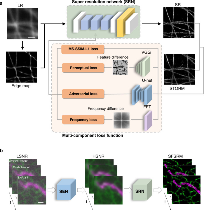
Fig. 1
The architecture of SFSRM.
a The super-resolution network (SRN) architecture. The SRN is trained with simulated low-resolution (LR) and ground-truth (GT) image pairs or experimental wide-field (WF) and STORM image pairs obtaine...
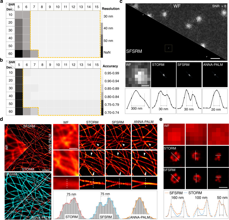
Fig. 2
Overview performance of SFSRM.
a , b The measured resolution and reconstruction accuracy of SFSRM on simulation line pairs at different signal densities (Den.) and SNRs. The orange dashed box indicates the applicable region of SFSR...
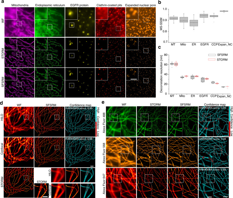
Fig. 3
SFSRM applies to different subcellular structures, imaging systems, and spectra.
a First row: representative WF images of mitochondria labeled with the mitochondrial membrane, endoplasmic reticulum (ER), EGFR protein after the EGF endocytosis, clathrin-coated pits after the EGF en...
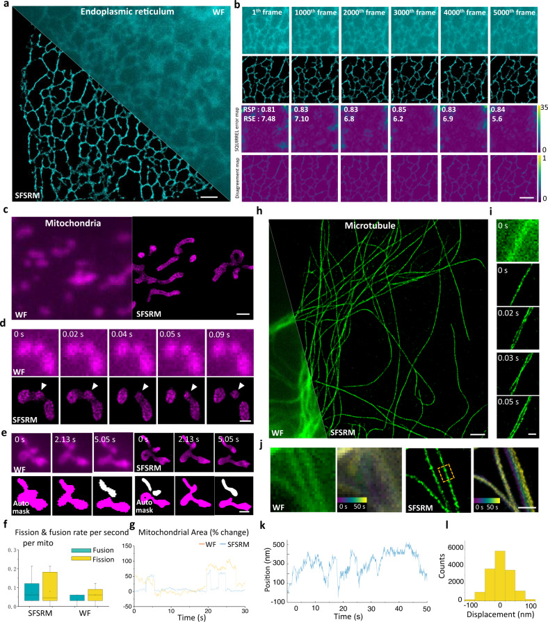
Fig. 4
SFSRM enables noninvasive super-resolution imaging in live cells at millisecond temporal resolution for thousands of frames.
a Representative WF and SFSRM images of endoplasmic reticulum in live Beas2B cells transfected with EGFP-Sec61u03b2. b Time-lapse images of endoplasmic reticulum in live cells imaged with 15u2009W/cm ...
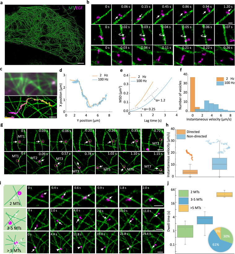
Fig. 5
Dual-color real-time SFSRM imaging reveals the microtubule-vesicle interactions.
a Representative dual-channel image of microtubules (green) and vesicles (magenta) in Beas2B cells after Epidermal Growth Factor (EGF) protein endocytosis. b Examples of vesicle transport dynamics. Fi...
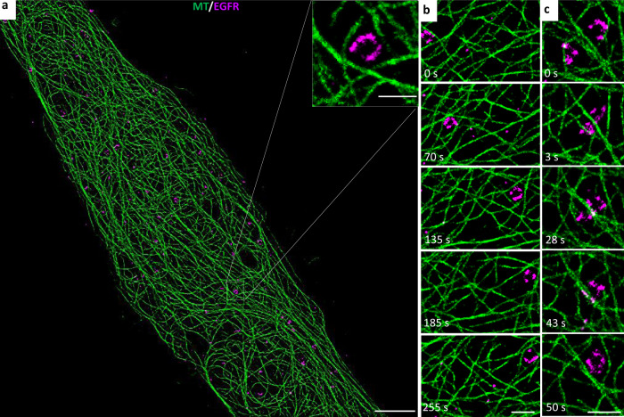
Fig. 6
SFSRM imaging allows long-time-scale observation.
a SFSRM reconstruction of a confocal image of microtubules (green) and EGFR-carrying vesicles (magenta) in Beas2B cells. Inset: an endosome accumulated with EGFR proteins is trapped in a local microtu...
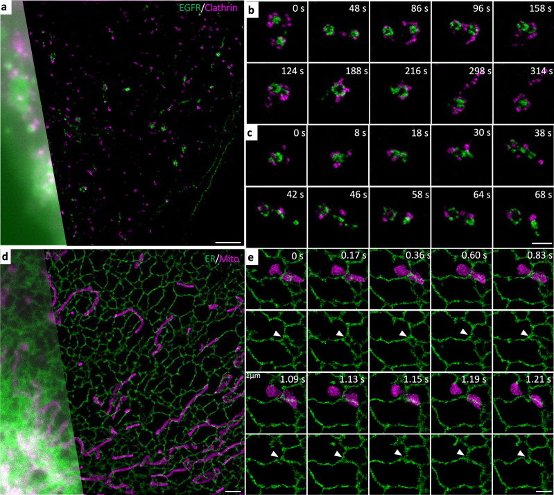
Fig. 7
Dual-color real-time SFSRM imaging reveals subcellular dynamics of diverse organelles.
a Representative dual-channel image of EGFR protein (green) and clathrin protein (magenta) in Beas2B cells expressing EGFR-EGFP and Halo-clathrin. b Example of the fusion process of two clathrin-coate...
Figure images are served from the NIH/NLM PubMed Central Open Access Subset or Europe PMC; copyright remains with the publishers and authors.
💬 Discussion
0 commentsNo comments yet. Be the first to start a discussion!
Leave a Comment