Abstract
AbstractStimulator of interferon genes (STING) is critical for the type I interferon response to pathogen- or self-derived DNA in the cytosol. STING may function as a scaffold to activate TANK-binding kinase 1 (TBK1), but direct cellular evidence remains lacking. Here we show, using single-molecule imaging of STING with enhanced time resolutions down to 5 ms, that STING becomes clustered at the trans-Golgi network (about 20 STING molecules per cluster). The clustering requires STING palmitoylation and the Golgi lipid order defined by cholesterol. Single-molecule imaging of TBK1 reveals that STING clustering enhances the association with TBK1. We thus provide quantitative proof-of-principle for the signaling STING scaffold, reveal the mechanistic role of STING palmitoylation in the STING activation, and resolve the long-standing question of the requirement of STING translocation for triggering the innate immune signaling.
🔬 Techniques
🔭 Microscopes
🧬 Organisms
💻 Software
✨ Fluorophores
🧪 Sample Preparation
🔬 Cell Lines
🏭 Microscope Brands
🧪 Reagent Suppliers
📷 Detectors
🔎 Objectives
🎨 Filters
💻 Software Details
🏛️ Research Organizations (ROR)
Affiliated research institutions:
📋 Methods
Antibodies
Antibodies used in this study were as follows: rabbit anti-STING (19851-1-AP, dilution 1:1000) and rabbit anti-calnexin (10427-2-AP, dilution 1:1000) (Proteintech); rabbit anti-phospho-STING (D8F4W, dilution 1:1000 for western blot), rabbit anti-phospho-TBK1 (D52C2, dilution 1:1000), rabbit anti-IRF3 (D83B9, dilution 1:1000), and rabbit anti-phospho-IRF3 (4D4G, dilution 1:1000) (Cell Signaling Technology); rabbit anti-TBK1 (ab40676, dilution 1:1000) (Abcam); mouse anti-α-tubulin (10G10, dilution 1:1000) and mouse anti-FLAG (1E6, dilution 1:1000) (Wako); mouse anti-CH25H (J2617, dilution 1:100; Santa Cruz); Goat anti-Rabbit IgG (H + L) Mouse/Human ads-HRP (4050-05, dilution 1:10,000) and Goat anti-Mouse IgG (H + L) Human ads-HRP (1031-05, dilution 1:10,000) (SouthernBiotech); sheep anti-TGN38 (AHP499G, dilution 1:200) (Bio-Rad); mouse anti-GM130 (610823, dilution 1:4000) (BD Biosciences); Alexa 568-, 594-, or 647-conjugated secondary antibodies (A10037, A11016, A21448, dilution 1:1000) (Thermo Fisher Scientific).
Reagents
The following reagents were purchased from the manufacturers as noted: DMXAA (14617, Cayman); di-4-ANEPPDHQ ( D36802 , Thermo Fisher Scientific); HaloTag® SaraFluor TM 650 T Ligand (A308-02, Goryo Chemical, Inc.), HaloTag® SaraFluor TM 650B Ligand (A201-01, Goryo Chemical, Inc.), D-ceramide-C6 (62525, Cayman); L-ceramide-C6 (24388, Cayman); MRT67307 (19916, Cayman); 2-Bromopalmitate (320-76562, Wako); HT-DNA (D6898, Sigma); Filipin III (70440, Cayman); 25-hydroxycholesterol (11097, Cayman); OSW-1 (30310, Cayman); Cholesterol, Water Soluble (C4951, Sigma); Dioleoyl phosphatidylcholine (850375, Avanti Polar Lipids); Cholesterol (C8667, Sigma); Lipi-Blue (LD01, DOJINDO). DMXAA was routinely used at 25 µg mL −1 throughout the present study. PCR cloning N -terminal mNeonGreen-, mRuby3-, or mEos4b-tagged mouse STING ( NM_028261 ) was introduced into pMXs-IPuro. C -terminal HaloTag7-tagged mouse TBK1 ( NM_019786 ), mouse GM130 ( NM_001080968.2 ), mouse TfnR (Transferrin Receptor) ( NM_011638.4 ), or mouse TGN38 ( NM_009443.3 ) was introduced into pMXs-IBla. C -terminal mScarletI-tagged human TBK1 ( NM_013254 ) was introduced into pMXs-IBla. N -terminal HaloTag7-tagged mouse Rab6a ( NM_024287 ) or mouse Rab11a ( NM_017382.5 ) was introduced into pMXs-IHyg. C -terminal FLAG-tagged mouse α-COP ( NM_009938.4 ) was introduced into pMXs-IBla. The cDNA plasmid encoding N-terminal mEos4b-tagged mouse cavin1 ( NM_008986.2 ) was produced by replacing GFP in the pEGFP-C1 vector (addgene, #68401) with mEos4b. The iD4H (D4 Y415A/D434S/A463W ) mutant fragment was generated by the standard two-step PCR mutagenesis technique using pCold I-GFPenvy-D4H (D4 D434S ) 66 as a template. The iD4H fragment was introduced into pMXs-IBla. To construct E. coli expression vector, mNeonGreen-iD4H fragment was amplified by PCR using pmNeonGreen-iD4H as a template and cloned into pCold I (Takara Bio, Shiga, Japan).
Show full methods section
Antibodies
Antibodies used in this study were as follows: rabbit anti-STING (19851-1-AP, dilution 1:1000) and rabbit anti-calnexin (10427-2-AP, dilution 1:1000) (Proteintech); rabbit anti-phospho-STING (D8F4W, dilution 1:1000 for western blot), rabbit anti-phospho-TBK1 (D52C2, dilution 1:1000), rabbit anti-IRF3 (D83B9, dilution 1:1000), and rabbit anti-phospho-IRF3 (4D4G, dilution 1:1000) (Cell Signaling Technology); rabbit anti-TBK1 (ab40676, dilution 1:1000) (Abcam); mouse anti-α-tubulin (10G10, dilution 1:1000) and mouse anti-FLAG (1E6, dilution 1:1000) (Wako); mouse anti-CH25H (J2617, dilution 1:100; Santa Cruz); Goat anti-Rabbit IgG (H + L) Mouse/Human ads-HRP (4050-05, dilution 1:10,000) and Goat anti-Mouse IgG (H + L) Human ads-HRP (1031-05, dilution 1:10,000) (SouthernBiotech); sheep anti-TGN38 (AHP499G, dilution 1:200) (Bio-Rad); mouse anti-GM130 (610823, dilution 1:4000) (BD Biosciences); Alexa 568-, 594-, or 647-conjugated secondary antibodies (A10037, A11016, A21448, dilution 1:1000) (Thermo Fisher Scientific).
Reagents
The following reagents were purchased from the manufacturers as noted: DMXAA (14617, Cayman); di-4-ANEPPDHQ ( D36802 , Thermo Fisher Scientific); HaloTag® SaraFluor TM 650 T Ligand (A308-02, Goryo Chemical, Inc.), HaloTag® SaraFluor TM 650B Ligand (A201-01, Goryo Chemical, Inc.), D-ceramide-C6 (62525, Cayman); L-ceramide-C6 (24388, Cayman); MRT67307 (19916, Cayman); 2-Bromopalmitate (320-76562, Wako); HT-DNA (D6898, Sigma); Filipin III (70440, Cayman); 25-hydroxycholesterol (11097, Cayman); OSW-1 (30310, Cayman); Cholesterol, Water Soluble (C4951, Sigma); Dioleoyl phosphatidylcholine (850375, Avanti Polar Lipids); Cholesterol (C8667, Sigma); Lipi-Blue (LD01, DOJINDO). DMXAA was routinely used at 25 µg mL −1 throughout the present study. PCR cloning N -terminal mNeonGreen-, mRuby3-, or mEos4b-tagged mouse STING ( NM_028261 ) was introduced into pMXs-IPuro. C -terminal HaloTag7-tagged mouse TBK1 ( NM_019786 ), mouse GM130 ( NM_001080968.2 ), mouse TfnR (Transferrin Receptor) ( NM_011638.4 ), or mouse TGN38 ( NM_009443.3 ) was introduced into pMXs-IBla. C -terminal mScarletI-tagged human TBK1 ( NM_013254 ) was introduced into pMXs-IBla. N -terminal HaloTag7-tagged mouse Rab6a ( NM_024287 ) or mouse Rab11a ( NM_017382.5 ) was introduced into pMXs-IHyg. C -terminal FLAG-tagged mouse α-COP ( NM_009938.4 ) was introduced into pMXs-IBla. The cDNA plasmid encoding N-terminal mEos4b-tagged mouse cavin1 ( NM_008986.2 ) was produced by replacing GFP in the pEGFP-C1 vector (addgene, #68401) with mEos4b. The iD4H (D4 Y415A/D434S/A463W ) mutant fragment was generated by the standard two-step PCR mutagenesis technique using pCold I-GFPenvy-D4H (D4 D434S ) 66 as a template. The iD4H fragment was introduced into pMXs-IBla. To construct E. coli expression vector, mNeonGreen-iD4H fragment was amplified by PCR using pmNeonGreen-iD4H as a template and cloned into pCold I (Takara Bio, Shiga, Japan).
Cell culture
MEFs were cultured in DMEM supplemented with 10% fetal bovine serum (FBS) and penicillin/streptomycin/glutamine (PSG) in a 5% CO 2 incubator. MEFs that stably express tagged proteins were established using retrovirus. Plat-E cells were transfected with pMXs vectors, and the medium that contains the retrovirus was collected. MEFs were incubated with the medium and then selected with puromycin (2 µg mL −1 ), blasticidin (5 µg mL −1 ), or hygromycin (400 µg mL −1 ) for several days. STING/TBK1- or STING/cGAS-double knockout MEFs were generated by CRISPR-Cas9 system 16 , 25 . Human prostate cancer (PC3; ATCC, CRL-1435) cells were cultured in HAM’s F12 supplemented with 10% FBS, 100 μ/ml penicillin, and 100 μg/ml streptomycin in a 5% CO2 incubator.
Immunocytochemistry
Cells were fixed with 4% paraformaldehyde (PFA) in PBS at room temperature for 15 min and permeabilized with 0.1% Triton X-100 in PBS at room temperature for 5 min. After blocking with 3% BSA in PBS, cells were incubated with primary antibodies. After washing with PBS three times, cells were then incubated with the secondary antibody at room temperature for 60 min, washed, and mounted with ProLong™ Glass Antifade Mountant ( P36982 , Thermo Fisher Scientific). For cholesterol staining, cells were fixed with 4% paraformaldehyde in PBS at room temperature for 15 min. After permeabilization by freeze-thawing with liquid nitrogen, cells were incubated with filipin III (50 µg mL −1 ) at room temperature for 30 min. For HaloTag7 staining, cells were fixed with 4% paraformaldehyde in PBS at room temperature for 15 min, and incubated with HaloTag® SaraFluor 650 T Ligand (1 µM) at room temperature for 30 min.
Fixed-cell imaging with confocal microscopy
Cells were seeded on coverslips (13 mm No.1 S, MATSUNAMI) the day before fixation. Confocal microscopy was performed using a LSM880 with Airyscan (Zeiss) with a 63 × 1.4 Plan-Apochromat oil immersion lens or 100 × 1.46 alpha-Plan-Apochromat oil immersion lens. Images were analyzed and processed with Zeiss ZEN 2.3 SP1 FP3 (black, 64-bit) (ver. 14.0.21.201) and Fiji (ver. 2.0.0-rc-69/1.52p). Pearson’s correlation coefficient was quantified by BIOP JACoP in Fiji plugin.
Live-cell imaging with confocal microscopy
Live-cell imaging was performed using LSM880 with Airyscan (Zeiss) equipped with a 100 × 1.46 alpha-Plan-Apochromat oil immersion lens and Immersol TM 518 F/37 °C (444970-9010-000, Zeiss). The day before imaging, cells were seeded on a glass bottom dish (627870, Greiner bio-one) with growth medium without phenol red. During live-cell imaging, the dish was mounted in a chamber (STXG-WSKMX-SET, TOKAI HIT) to maintain the incubation conditions at 37 °C and 5% CO 2 . Images were acquired at intervals of 6 s, analyzed and Airyscan processed with Zeiss ZEN 2.3 SP1 FP3 (black, 64 bit) (ver. 14.0.21.201) and Fiji (ver. 2.0.0-rc-69/1.52p). For HaloTag7 staining before live-cell imaging, cells were cultured in medium containing HaloTag7 ligand at 37 °C for 30 min in a 5% CO 2 incubator. In vitro assay of recombinant TBK1-dependent phosphorylation of STING Cells were collected in an ice-cold buffer (50 mM Tris–HCl pH 7.4, 100 mM NaCl, 1 mM EGTA, 2 mM DTT, 200 mM sucrose) containing protease inhibitors (25955-11, nacalai tesque), and phosphatase inhibitors (8 mM NaF, 12 mM β-glycerophosphate, 1 mM Na 3 VO 4 , 1.2 mM Na 2 MoO 4 , 5 μM cantharidin, and 2 mM imidazole), homogenized with 2 passages through a 27-gauge needle after 6 passages through a 23-gauge needle and centrifuged at 3000 × g for 5 min at 4 °C. The post-nuclear supernatant was overlaid on 10 μL of 2 M sucrose and centrifuged at 100,000 × g for 1 h at 4 °C. The membrane fractions were resuspended in a buffer (50 mM Tris–HCl pH 7.4, 100 mM NaCl, 1 mM EGTA, 2 mM DTT, 200 mM sucrose, 20 mM MgCl 2 , protease inhibitors, and phosphatase inhibitors), and incubated with ATP (1 mM) and recombinant TBK1 (100 ng) at 37 °C for 30 min. The samples were then subjected to SDS-PAGE and phosphorylation of STING was detected by western blot.
Liposome co-sedimentation assay
Recombinant mNeonGreen-iD4H protein was expressed in E. coli and purified with Ni-NTA (Qiagen) according to the manufacturer’s protocol 67 . Lipid mixtures (Dioleoyl phosphatidylcholine and cholesterol) were dried under nitrogen gas and hydrated in buffer A (20 mM HEPES-NaOH (pH 7.4), 100 mM sucrose, 100 mM KCl, and 1 mM EDTA) for 15 min at room temperature, and vortexed briefly. mNeonGreen-iD4H recombinant protein was diluted with HEPES Buffered Saline, incubated with the liposomes in buffer A for 30 min at 30 °C. The mixture was centrifuged at 20,000 x g for 30 min at 25 °C. The resultant supernatant was collected, and the pellet was washed twice with buffer A. The pellet was then subjected to SDS-PAGE and Coomassie Brilliant Blue (CBB) Staining.
Measurement of lipid order using di-4-ANEPPDHQ
Cells were incubated with di-4-ANEPPDHQ (1 µg mL −1 ) in DMEM at 37 °C for 30 min followed by image acquisition. All images for di-4-ANEPPDHQ were acquired on LSM880 (Zeiss) with a 488 nm Ar laser and a 633 nm He-Ne laser line using a 63 × 1.4 Plan-Apochromat oil immersion lens. di-4-ANEPPDHQ was excited at 488 nm, and the emissions were captured at the following manual bandwidth settings of the spectral detection channel: Ch-L, 505–530 nm; and Ch-H, 675–700 nm. The SaraFluor TM 650 T was excited at 633 nm and detected with the spectral detector at 670–750 nm. di-4-ANEPPDHQ intensity images were converted into generalized polarization (GP) images 41 , with each pixel calculated in Fiji from the two di-4-ANEPPDHQ intensity images according to the equation: GP = ( I Ch-L – I Ch-H ) / ( I Ch-L + I Ch-H ). GP values in the Golgi area or TBK1 foci were obtained by using binarized images of HaloTag7-Rab6 or TBK1-HaloTag7 generated by Trainable Weka Segmentation, a machine learning tool for microscopy pixel classification in Fiji plugin. GP values in the cytoplasm without plasma membrane were obtained by measuring the mean of GP values in a region 2 µm inside the cell edge. qRT-PCR Total RNA was reverse-transcribed by using ReverTraAce qPCR RT Master Mix with gDNA Remover (TOYOBO). Quantitative real-time PCR (qRT-PCR) was performed using KOD SYBR qPCR (TOYOBO) and LightCycler 96 (Roche). The sequences of the primers were as follows. 5’-AGTGCTGCCGTCATTTTCTGCCTC-3’ (mouse Cxcl10; sense primer) and 5’-GCAGGATAGGCTCGCAGGGATGATT-3’ (mouse Cxcl10; antisense primer); 5’-AGGTCGGTGTGAACGGATTTG-3’ (mouse Gapdh; sense primer) and 5’-TGTAGACCATGTAGTTGAGGTCA-3’ (mouse Gapdh; antisense primer). Target gene expression was normalized based on Gapdh content.
Lipid analysis
Cells were collected in an ice-cold buffer (50 mM Tris–HCl pH 7.4, 100 mM NaCl, 1 mM EGTA, 2 mM DTT, 200 mM sucrose) containing protease inhibitors (25955-11, nacalai tesque), and phosphatase inhibitors (8 mM NaF, 12 mM β-glycerophosphate, 1 mM Na 3 VO 4 , 1.2 mM Na 2 MoO 4 , 5 µM cantharidin, and 2 mM imidazole), homogenized with 2 passages through a 27-gauge needle after 6 passages through a 23-gauge needle, and centrifuged at 3000 × g for 5 min at 4 °C. The post-nuclear supernatant was overlaid on 10 µL of 2 M sucrose and centrifuged at 100,000 × g for 1 h at 4 °C. Total lipids were extracted by the Bligh and Dyer method 68 . To detect cholesterol, lipid extracts were subjected to high-performance TLC (Merck) separation with hexane/diethyl ether/ acetic acid (80:20:1, vol:vol:vol). Cholesterols were stained with a mixture of ferric chloride/sulfuric acid/acetic acid by heating 69 . RNA interference siRNA specific to Ch25h (Ch25h Stealth Select RNAi) purchased from Thermo Fisher Scientific. Negative control siRNA was purchased from Dharmacon. A total of 5 nM siRNA was introduced to cells using Lipofectamine RNAiMAX (Invitrogen) according to the manufacturer’s instruction. Cells were further incubated for 72 h for subsequent experiments. Cholesterol add-back experiments Cells were incubated with medium containing cholesterol-methyl-β-cyclodextrin complex (Chol/MβCD) (3.9 mM) for 3 h.
Statistical analysis
Error bars displayed in bar plots throughout this study represent s.e.m. unless otherwise indicated and were calculated from triplicate or quadruplicate samples. In box-and-whisker plots, the box bounds the interquartile range (IQR) divided by the median, and whiskers extend to a maximum of 1.5 × IQR beyond the box. The corresponding data points are overlayed on the plots. The data were statistically analyzed by performing one-way ANOVA followed by Tukey-Kramer post hoc test with KNIME (4.6.3) and R (4.0.2). The number of STING molecules per cluster and the number of STING molecules within 100 nm radius around TBK1 spots were statistically analyzed by performing Welch’s t -test (both-sided). In cases requiring multiple statistical tests, the significance level was corrected by the Holm-Sidak method. When the histogram of colocalization durations was fitted with a single exponential decay function, the 68.3% confidence limit was given as the fitting error for the decay time. The statistical analysis for these distributions was performed using log-rank test (statistical survival analysis). The significance level was corrected by the Holm-Sidak method.
Data acquisition of live-cell PALM of mEos4b-STING or mEos4b-cavin1
For live-cell PALM observation of mEos4b-STING, MEFs were sparsely seeded in a glass-base dish (4 × 10 3 cells on the glass window of 12 mm in diameter, 0.15-mm-thick glass; Iwaki), and grown in DMEM without phenol red supplemented with 10% FBS for 2 days before each experiment. The data acquisitions of PALM of mEos4b-STING were performed at 37 °C and at a video rate (33 ms/frame) or 5 ms/frame for 5400 frames with an image size of 1024 × 1024 pixels or 512 × 512 pixels, respectively, using an Olympus IX-83 inverted microscope (100 × 1.50 NA oil objective) equipped with a high-speed gate image intensifier (C9016-02MLG; Hamamatsu Photonics) coupled to an sCMOS camera (OCRA-Flash4.0 V2; Hamamatsu Photonics). mEos4b-STING molecules in cells were illuminated with the oblique-angle illumination mode using an activation laser (405 nm, approximately 4 nW/µm 2 and 20 nW/µm 2 for observation at 33 ms/frame and 5 ms/frame, respectively) and an excitation laser (561 nm, approximately 7 µW/µm 2 and 14 µW/µm 2 for observation at 33 ms/frame and 5 ms/frame, respectively). The single-molecule localization precision of mEos4b was 20 ± 1 nm. The final magnifications were 133×, resulting in pixel sizes of 47.1 nm (square pixels). For live-cell PALM observation of mEos4b-cavin1, PC3 cells were transfected with cDNA encoding mEos4b-cavin1 by 4D-nucleofector (LONZA) and the cells were sparsely seeded in a glass-base dish, and grown in HAM/F12 with 10% FBS for 2 days before observation. The data acquisitions of PALM of mEos4b-cavin1 were performed at 37 °C and at a video rate (33 ms/frame) with an image size of 1024 × 1024 pixels. Single mEos4b-cavin1 molecules in cells were observed by total internal reflection microscopy. In vitro blinking observation of immobilized mEos4b and analysis For correction of multiple blinking of mEos4b, we observed in vitro blinking and photoactivation behaviors of purified mEos4b. mEos4b gene was cloned in the pET15b plasmid, transformed in E coli , BL21 (DE3) to overexpress proteins, and mEos4b was purified using a His60 Ni Superflow Cartridge Purification Kit (Clontech), followed by a gel-filtration step using a PD-10 column (Cytiva). The purified mEos4b was diluted to 5 nM in a solution of 1% polyvinyl alcohol (PVA, nacalai tesque) in HBSS (pH = 7.4). Then, 150 µl of the mEos4b solution was placed in a glass window of the glass base dish and was incubated for 1 h at room temperature to form a uniform thin layer. After washing with HBSS, 1 ml HBSS was added to the dish. The blinking and photoactivation behaviors of mEos4b molecules were observed under the same laser illumination condition as that in cells. As shown in Fig. 1b , we observed single mEos4b molecule emission trace, and measured the number of times mEos4b blinks before a photobleaching event, the fluorescence-on time (T on ) before the molecule goes into the dark state or it photobleaches, the fluorescence-off time (T off ) or the time the molecule spends in the dark state as previously reported 27 . The estimation of these parameters from the obtained images of mEos4b immobilized in PVA was performed by using the GDSC SMLM plugin of ImageJ (Time threshold was set to 2.5 s). The histogram of relationship between and the probability was fitted by the predicted geometric distribution; 1 documentclass[12pt]{minimal} usepackage{amsmath} usepackage{wasysym} usepackage{amsfonts} usepackage{amssymb} usepackage{amsbsy} usepackage{mathrsfs} usepackage{upgreek} setlength{oddsidemargin}{-69pt} begin{document}$${{{{{rm{P}}}}}}({{{{{rm{N}}}}}}_{{{{{rm{blink}}}}}}={{n}})={{{{{rm{h}}}}}}{^{n}}(1-{{{{{rm{h}}}}}})$$end{document} P ( N blink = n ) = h n ( 1 − h ) where h = k d /(k d +k b ) is the probability of transition to the dark state and k d and k b are the rates of transition to the dark and the photobleach states, respectively (Fig. 1d ). The histogram of relationship between T on and probability density function (PDF) was fitted with single exponential decay function, providing k b + k d (Fig. 1e ). N blink (= k d /k b ) was estimated from these values.
Analysis of images obtained by super-resolution microscopy
The detection of the fluorescent spots in the images was performed by using the ThunderSTORM plugin of ImageJ with “Wavelet filtering” (B-Spline order = 6 and B-Spline scale = 6.0) and the “Local maximum method” (Peak intensity threshold = 30−50 and Connectivity = 8-neighborhood). After spot detection, the post-processing steps of “Remove duplications” (Distance threshold = uncertainty) and “Drift correction” (cross-correlation with 5 bins) were further performed. Several methods for PALM image segmentation have been proposed, but which method is the most appropriate is under debate and depends on characteristics of the objects of observation such as molecular density, cluster size, and the ratio of molecules in clusters to those in bulk phase, etc 32 . For example, a pair-correlation method identifies molecular interactions inside clusters by analyzing distance correlation between localizations, but this method does not give us the number and position of clusters, and can be applied only to small clusters of relatively homogenous sizes. Density based spatial clustering analysis with noise (DBSCAN), which allows the classification of molecules in clusters, is known to be sensitive to background noise and difficult to parameterize experimentally. In the present study, we employed two kinds of ways for the image segmentation to detect mEos4b-STING clusters, kernel density estimation (KDE) and SR-Tesseler. In these methods, image segmentation is performed directly from the localization coordinates, which is applicable for the analysis of clusters of heterogenous size, and insensitive to background noise. Furthermore, these methods can be applicable to a wide range of the objects of observation 32 . SR-Tessler 34 is one of the most frequently used methods for PALM image segmentation. Meanwhile, KDE 31 , 70 is a traditional image segmentation method and can rapidly determine the criterion for segmenting PLAM images as reported previously 71 and described below. KDE provides a way to interpolate object boundaries without bias by the random fluctuations of activated boundary fluorophores. In this study, the binarized PALM images of STING clusters were used for estimation of the residency time of single-molecules of TBK1-HaloTag7 inside the STING clusters upon stimulation (Fig. 8d, e ). The datasets obtained by Thunderstorm were imported to the KDE software (MATLAB) for the cluster analysis and the image reconstruction. We used not only localization coordinates, but also uncertainty outputted by Thunderstorm, which represents the degree of spatial precision of the spot. Let documentclass[12pt]{minimal} usepackage{amsmath} usepackage{wasysym} usepackage{amsfonts} usepackage{amssymb} usepackage{amsbsy} usepackage{mathrsfs} usepackage{upgreek} setlength{oddsidemargin}{-69pt} begin{document}$${x}_{i},{y}_{i}$$end{document} x i , y i , and documentclass[12pt]{minimal} usepackage{amsmath} usepackage{wasysym} usepackage{amsfonts} usepackage{amssymb} usepackage{amsbsy} usepackage{mathrsfs} usepackage{upgreek} setlength{oddsidemargin}{-69pt} begin{document}$${u}_{i},{i}={{{{mathrm{1,2}}}}},cdots,N$$end{document} u i , i = 1, 2 , ⋯ , N be the horizontal and vertical localization coordinates and uncertainty of spot documentclass[12pt]{minimal} usepackage{amsmath} usepackage{wasysym} usepackage{amsfonts} usepackage{amssymb} usepackage{amsbsy} usepackage{mathrsfs} usepackage{upgreek} setlength{oddsidemargin}{-69pt} begin{document}$$i$$end{document} i , respectively. documentclass[12pt]{minimal} usepackage{amsmath} usepackage{wasysym} usepackage{amsfonts} usepackage{amssymb} usepackage{amsbsy} usepackage{mathrsfs} usepackage{upgreek} setlength{oddsidemargin}{-69pt} begin{document}$$N$$end{document} N represents the total number of spots. Considering the uncertainty of the location measurement of spot documentclass[12pt]{minimal} usepackage{amsmath} usepackage{wasysym} usepackage{amsfonts} usepackage{amssymb} usepackage{amsbsy} usepackage{mathrsfs} usepackage{upgreek} setlength{oddsidemargin}{-69pt} begin{document}$$i$$end{document} i , it is considered that the existence probability documentclass[12pt]{minimal} usepackage{amsmath} usepackage{wasysym} usepackage{amsfonts} usepackage{amssymb} usepackage{amsbsy} usepackage{mathrsfs} usepackage{upgreek} setlength{oddsidemargin}{-69pt} begin{document}$${p}_{i}left(x,yright)$$end{document} p i x , y of the spot documentclass[12pt]{minimal} usepackage{amsmath} usepackage{wasysym} usepackage{amsfonts} usepackage{amssymb} usepackage{amsbsy} usepackage{mathrsfs} usepackage{upgreek} setlength{oddsidemargin}{-69pt} begin{document}$$i$$end{document} i spreads to the Gaussian distribution with the center coordinate documentclass[12pt]{minimal} usepackage{amsmath} usepackage{wasysym} usepackage{amsfonts} usepackage{amssymb} usepackage{amsbsy} usepackage{mathrsfs} usepackage{upgreek} setlength{oddsidemargin}{-69pt} begin{document}$${x}_{i},{y}_{i}$$end{document} x i , y i and the standard deviation (S.D.) that is proportional to the uncertainty documentclass[12pt]{minimal} usepackage{amsmath} usepackage{wasysym} usepackage{amsfonts} usepackage{amssymb} usepackage{amsbsy} usepackage{mathrsfs} usepackage{upgreek} setlength{oddsidemargin}{-69pt} begin{document}$${u}_{i}$$end{document} u i as follows: 2 documentclass[12pt]{minimal} usepackage{amsmath} usepackage{wasysym} usepackage{amsfonts} usepackage{amssymb} usepackage{amsbsy} usepackage{mathrsfs} usepackage{upgreek} setlength{oddsidemargin}{-69pt} begin{document}$${p}_{i}left(x,yright)=frac{1}{2pi {(A{u}_{i})}^{2}}{e}^{-frac{{(x-{x}_{i})}^{2}+{(y-{y}_{i})}^{2}}{2{(A{u}_{i})}^{2}}}$$end{document} p i x , y = 1 2 π ( A u i ) 2 e − ( x − x i ) 2 + ( y − y i ) 2 2 ( A u i ) 2 in which, documentclass[12pt]{minimal} usepackage{amsmath} usepackage{wasysym} usepackage{amsfonts} usepackage{amssymb} usepackage{amsbsy} usepackage{mathrsfs} usepackage{upgreek} setlength{oddsidemargin}{-69pt} begin{document}$$A$$end{document} A is the proportional coefficient of S.D. to the uncertainty documentclass[12pt]{minimal} usepackage{amsmath} usepackage{wasysym} usepackage{amsfonts} usepackage{amssymb} usepackage{amsbsy} usepackage{mathrsfs} usepackage{upgreek} setlength{oddsidemargin}{-69pt} begin{document}$${u}_{i}$$end{document} u i ; that is estimated as documentclass[12pt]{minimal} usepackage{amsmath} usepackage{wasysym} usepackage{amsfonts} usepackage{amssymb} usepackage{amsbsy} usepackage{mathrsfs} usepackage{upgreek} setlength{oddsidemargin}{-69pt} begin{document}$$Aapprox 6$$end{document} A ≈ 6 by some preliminary experiments. Gaussian distribution constructing each existence probability documentclass[12pt]{minimal} usepackage{amsmath} usepackage{wasysym} usepackage{amsfonts} usepackage{amssymb} usepackage{amsbsy} usepackage{mathrsfs} usepackage{upgreek} setlength{oddsidemargin}{-69pt} begin{document}$${p}_{i}left(x,yright)$$end{document} p i x , y is called Gaussian kernel. The existence probability distribution for all spots, i.e., the PALM image is obtained by the average of the existence probability distribution documentclass[12pt]{minimal} usepackage{amsmath} usepackage{wasysym} usepackage{amsfonts} usepackage{amssymb} usepackage{amsbsy} usepackage{mathrsfs} usepackage{upgreek} setlength{oddsidemargin}{-69pt} begin{document}$${p}_{i}left(x,yright)$$end{document} p i x , y as 3 documentclass[12pt]{minimal} usepackage{amsmath} usepackage{wasysym} usepackage{amsfonts} usepackage{amssymb} usepackage{amsbsy} usepackage{mathrsfs} usepackage{upgreek} setlength{oddsidemargin}{-69pt} begin{document}$$pleft(x,yright)=frac{1}{N}mathop{sum }limits_{i=1}^{N}{p}_{i}left(x,yright)$$end{document} p x , y = 1 N ∑ i = 1 N p i x , y excluding spots having extremely small or large uncertainty documentclass[12pt]{minimal} usepackage{amsmath} usepackage{wasysym} usepackage{amsfonts} usepackage{amssymb} usepackage{amsbsy} usepackage{mathrsfs} usepackage{upgreek} setlength{oddsidemargin}{-69pt} begin{document}$${u}_{i}$$end{document} u i because such spots are likely to be noise. It can be considered that clusters exist where the PALM image, which represents the cluster existence probability distribution, takes above a certain threshold value documentclass[12pt]{minimal} usepackage{amsmath} usepackage{wasysym} usepackage{amsfonts} usepackage{amssymb} usepackage{amsbsy} usepackage{mathrsfs} usepackage{upgreek} setlength{oddsidemargin}{-69pt} begin{document}$$theta$$end{document} θ because the spots appear uniformly inside the clusters with a certain probability. It is necessary to appropriately determine the optimal threshold value documentclass[12pt]{minimal} usepackage{amsmath} usepackage{wasysym} usepackage{amsfonts} usepackage{amssymb} usepackage{amsbsy} usepackage{mathrsfs} usepackage{upgreek} setlength{oddsidemargin}{-69pt} begin{document}$$theta$$end{document} θ for each obtained PALM image because the optimal value differs depending on the target molecule and the experimental environments. In general, the histogram of documentclass[12pt]{minimal} usepackage{amsmath} usepackage{wasysym} usepackage{amsfonts} usepackage{amssymb} usepackage{amsbsy} usepackage{mathrsfs} usepackage{upgreek} setlength{oddsidemargin}{-69pt} begin{document}$$p(x,y)$$end{document} p ( x , y ) values for all documentclass[12pt]{minimal} usepackage{amsmath} usepackage{wasysym} usepackage{amsfonts} usepackage{amssymb} usepackage{amsbsy} usepackage{mathrsfs} usepackage{upgreek} setlength{oddsidemargin}{-69pt} begin{document}$$x,{y}$$end{document} x , y forms a bimodal shape consisting of both larger values created by dense spots appeared in clusters and smaller values created by sporadic noise. Therefore, the threshold value documentclass[12pt]{minimal} usepackage{amsmath} usepackage{wasysym} usepackage{amsfonts} usepackage{amssymb} usepackage{amsbsy} usepackage{mathrsfs} usepackage{upgreek} setlength{oddsidemargin}{-69pt} begin{document}$$theta$$end{document} θ should be determined so as to separate these two clusters. Otsu’s method is well known as a method for determining such a threshold value 72 . Let documentclass[12pt]{minimal} usepackage{amsmath} usepackage{wasysym} usepackage{amsfonts} usepackage{amssymb} usepackage{amsbsy} usepackage{mathrsfs} usepackage{upgreek} setlength{oddsidemargin}{-69pt} begin{document}$${S}_{{in}}$$end{document} S i n and documentclass[12pt]{minimal} usepackage{amsmath} usepackage{wasysym} usepackage{amsfonts} usepackage{amssymb} usepackage{amsbsy} usepackage{mathrsfs} usepackage{upgreek} setlength{oddsidemargin}{-69pt} begin{document}$${S}_{{out}}$$end{document} S o u t be sets of coordinates documentclass[12pt]{minimal} usepackage{amsmath} usepackage{wasysym} usepackage{amsfonts} usepackage{amssymb} usepackage{amsbsy} usepackage{mathrsfs} usepackage{upgreek} setlength{oddsidemargin}{-69pt} begin{document}$$(x,y)$$end{document} ( x , y ) where documentclass[12pt]{minimal} usepackage{amsmath} usepackage{wasysym} usepackage{amsfonts} usepackage{amssymb} usepackage{amsbsy} usepackage{mathrsfs} usepackage{upgreek} setlength{oddsidemargin}{-69pt} begin{document}$$p(x,y)ge theta$$end{document} p ( x , y ) ≥ θ and documentclass[12pt]{minimal} usepackage{amsmath} usepackage{wasysym} usepackage{amsfonts} usepackage{amssymb} usepackage{amsbsy} usepackage{mathrsfs} usepackage{upgreek} setlength{oddsidemargin}{-69pt} begin{document}$$pleft(x,yright) < theta$$end{document} p x , y < θ , respectively. The sets documentclass[12pt]{minimal} usepackage{amsmath} usepackage{wasysym} usepackage{amsfonts} usepackage{amssymb} usepackage{amsbsy} usepackage{mathrsfs} usepackage{upgreek} setlength{oddsidemargin}{-69pt} begin{document}$${S}_{{in}}$$end{document} S i n and documentclass[12pt]{minimal} usepackage{amsmath} usepackage{wasysym} usepackage{amsfonts} usepackage{amssymb} usepackage{amsbsy} usepackage{mathrsfs} usepackage{upgreek} setlength{oddsidemargin}{-69pt} begin{document}$${S}_{{out}}$$end{document} S o u t mean the inside and outside of clusters, respectively. The number of elements of the sets documentclass[12pt]{minimal} usepackage{amsmath} usepackage{wasysym} usepackage{amsfonts} usepackage{amssymb} usepackage{amsbsy} usepackage{mathrsfs} usepackage{upgreek} setlength{oddsidemargin}{-69pt} begin{document}$${S}_{{in}}$$end{document} S i n and documentclass[12pt]{minimal} usepackage{amsmath} usepackage{wasysym} usepackage{amsfonts} usepackage{amssymb} usepackage{amsbsy} usepackage{mathrsfs} usepackage{upgreek} setlength{oddsidemargin}{-69pt} begin{document}$${S}_{{out}}$$end{document} S o u t are respectively represented by documentclass[12pt]{minimal} usepackage{amsmath} usepackage{wasysym} usepackage{amsfonts} usepackage{amssymb} usepackage{amsbsy} usepackage{mathrsfs} usepackage{upgreek} setlength{oddsidemargin}{-69pt} begin{document}$${N}_{{in}}$$end{document} N i n and documentclass[12pt]{minimal} usepackage{amsmath} usepackage{wasysym} usepackage{amsfonts} usepackage{amssymb} usepackage{amsbsy} usepackage{mathrsfs} usepackage{upgreek} setlength{oddsidemargin}{-69pt} begin{document}$${N}_{{out}}$$end{document} N o u t . The intra-class variances of the sets documentclass[12pt]{minimal} usepackage{amsmath} usepackage{wasysym} usepackage{amsfonts} usepackage{amssymb} usepackage{amsbsy} usepackage{mathrsfs} usepackage{upgreek} setlength{oddsidemargin}{-69pt} begin{document}$${S}_{{in}}$$end{document} S i n and documentclass[12pt]{minimal} usepackage{amsmath} usepackage{wasysym} usepackage{amsfonts} usepackage{amssymb} usepackage{amsbsy} usepackage{mathrsfs} usepackage{upgreek} setlength{oddsidemargin}{-69pt} begin{document}$${S}_{{out}}$$end{document} S o u t are calculated by 4 documentclass[12pt]{minimal} usepackage{amsmath} usepackage{wasysym} usepackage{amsfonts} usepackage{amssymb} usepackage{amsbsy} usepackage{mathrsfs} usepackage{upgreek} setlength{oddsidemargin}{-69pt} begin{document}$${sigma }^{2}left[{S}_{{in}}right]=frac{1}{{N}_{{in}}}mathop{sum}limits_{left(x,yright)in {S}_{{in}}}pleft(x,yright)$$end{document} σ 2 S i n = 1 N i n ∑ x , y ∈ S i n p x , y 5 documentclass[12pt]{minimal} usepackage{amsmath} usepackage{wasysym} usepackage{amsfonts} usepackage{amssymb} usepackage{amsbsy} usepackage{mathrsfs} usepackage{upgreek} setlength{oddsidemargin}{-69pt} begin{document}$${sigma }^{2}left[{S}_{{out}}right]=frac{1}{{N}_{{out}}}mathop{sum}limits_{left(x,yright)in {S}_{{out}}}pleft(x,yright)$$end{document} σ 2 S o u t = 1 N o u t ∑ x , y ∈ S o u t p x , y The average of these intra-class variances is 6 documentclass[12pt]{minimal} usepackage{amsmath} usepackage{wasysym} usepackage{amsfonts} usepackage{amssymb} usepackage{amsbsy} usepackage{mathrsfs} usepackage{upgreek} setlength{oddsidemargin}{-69pt} begin{document}$${sigma }^{2}left[{S}_{{in}},{S}_{{out}}right]=frac{{N}_{{in}}{sigma }^{2}left[{S}_{{in}}right]+{N}_{{out}}{sigma }^{2}left[{S}_{{out}}right]}{{N}_{{in}}+{N}_{{out}}}$$end{document} σ 2 S i n , S o u t = N i n σ 2 S i n + N o u t σ 2 S o u t N i n + N o u t The Otsu’s method determines the optimal threshold value documentclass[12pt]{minimal} usepackage{amsmath} usepackage{wasysym} usepackage{amsfonts} usepackage{amssymb} usepackage{amsbsy} usepackage{mathrsfs} usepackage{upgreek} setlength{oddsidemargin}{-69pt} begin{document}$$hat{theta }$$end{document} θ ^ so as to minimize the average of the intra-class variances documentclass[12pt]{minimal} usepackage{amsmath} usepackage{wasysym} usepackage{amsfonts} usepackage{amssymb} usepackage{amsbsy} usepackage{mathrsfs} usepackage{upgreek} setlength{oddsidemargin}{-69pt} begin{document}$${sigma }^{2}left[{S}_{{in}},{S}_{{out}}right]$$end{document} σ 2 S i n , S o u t as follows: 7 documentclass[12pt]{minimal} usepackage{amsmath} usepackage{wasysym} usepackage{amsfonts} usepackage{amssymb} usepackage{amsbsy} usepackage{mathrsfs} usepackage{upgreek} setlength{oddsidemargin}{-69pt} begin{document}$$hat{theta }={{arg }}mathop{min }limits_{theta }{sigma }^{2}[{S}_{{i}n},, {S}_{out}]$$end{document} θ ^ = arg min θ σ 2 [ S i n , S o u t ] In this study, the clusters are determined using the above Otsu’s method. Alternatively, the dataset obtained by Thunderstorm was also imported to the SR-Tesseler software for the cluster analysis and image reconstruction 34 . Cluster contour detection was performed by using a Voronoi polygon density factor of 2 without correction of blinking and multi-ON frame detections by the”Detection cleaner” function (within the whole ROI). Multiple blinking effects were corrected by two methods. One of them is the most commonly used method to merge events that appear close in space and time which is referred to as dark-time thresholding (DTT) 27 . To estimate the numbers of mEos4b-STING in clusters, the numbers of localizations in clusters obtained by the KDE or SR-Tesseler method were divided by 1 + , which is the number of localizations per one mEos4b molecule (2.7 for observation at 33 ms/frame and 2.9 for observation at 5 ms/frame observation). The previous study demonstrated 27 that this method accomplishes unbiased counting of molecules in clusters. DTT has been most commonly used for the correction of multiple-blinking, but we need to assume that the blinking behaviors of isolated mEos4b are maintained also in cells. Therefore, to validate the STING numbers per cluster, we also corrected multiple-blinking artifacts by another method, using the PALM dataset and the parameters of a realistic model of fluorescent protein photophysics, which was recently reported and referred to as model-based correction (MBC) 35 . MBC requires neither user input nor additional calibration data.
Using two methods of PALM image segmentation
(KDE and SR-Tesseler) and two methods of multiple-blinking correction (division by 1 + and MBC), we estimated averaged numbers of mEos4b-STING in clusters by three ways. Namely, we performed PALM image segmentation and multiple-blinking correction in the following three ways; (1) The number of localizations segmented by KDE was divided by 1 + , (2) The number of localizations segmented by SR-Tesseller was divided by 1 + , (3) mEos4b-STING spots corrected by MBC was segmented by SR-Tessler. Simultaneous dual-color observation of live-cell PALM of mEos4b-STING and dSTORM of GM130-HaloTag7, TGN38-HaloTag7, TfnR-HaloTag7 or HaloTag7-Rab11 and coordinate-based colocalization analysis of PALM and dSTORM data Simultaneous data acquisitions of live-cell PALM of mEos4b-STING and dSTORM of GM130-HaloTag7 (a CGN protein), TGN38-HaloTag7 (a TGN protein), TfnR-HaloTag7 (an endosome protein) or HaloTag7-Rab11 (an endosome protein) were performed at 5 ms resolution and at 37 °C. The data acquisition of PALM of mEos4b-STING was performed as described in the method section of “Data acquisition of live-cell PALM of mEos4b-STING”. For live-cell dSTORM of GM130-HaloTag7, TGN38-HaloTag7, TfnR-HaloTag7 or HaloTag7-Rab11, these molecules expressed in cells and labeled with SaraFluor650B (SF650B) were illuminated with the oblique-angle illumination mode using an excitation laser (647 nm, approximately 16 µW/µm 2 ). In the excitation arm, a multiple-band mirror (ZT405/488/561/647rpc, Chroma) was employed. The two-color fluorescence images of mEos4b and SF650B were separated into the two detection arms of the microscope by a dichroic mirror (Chroma: ZT561rdc-xr-UF2 or ZT647rdc-UF2). The detection arms were equipped with band-pass filters of FF01-600/37-25 (Semrock) or ET700/75 (Chroma), and the data acquisitions of PALM/dSTROM were performed at 5 ms/frame with an image size of 512 × 512 pixels, using two high-speed gate image intensifiers (C9016-02MLG; Hamamatsu Photonics) coupled to two sCMOS cameras (OCRA-Flash4.0 V2; Hamamatsu Photonics). The superimposition of images in different colors obtained by two separate cameras was performed as reported previously 73 . To quantitatively analyze the degree of colocalization between mEos4b-STING and GM130-HaloTag7-SF650B, TGN38-HaloTag7-SF650B, TfnR-HaloTag7-SF650B, or SF650B-HaloTag7-Rab11, we performed coordinate-based colocalization (CBC) analysis of PLAM and dSTORM data according to ref. 36 . with modification. Briefly, to estimate CBC values, for each molecule of protein A, the number of localizations of protein A (mEos4b-STING) and protein B (GM130-HaloTag7-SF650B, TGN38-HaloTag7-SF650B, TfnR-HaloTag7-SF650B, or SF650B-HaloTag7-Rab11) within circles of the increasing radius was calculated, respectively, providing the density gradients of localizations of protein A and protein B around this molecule. 8 documentclass[12pt]{minimal} usepackage{amsmath} usepackage{wasysym} usepackage{amsfonts} usepackage{amssymb} usepackage{amsbsy} usepackage{mathrsfs} usepackage{upgreek} setlength{oddsidemargin}{-69pt} begin{document}$${D}_{{{{{{rm{Ai}}}}}},{{{{{rm{A}}}}}}}({{{{{rm{r}}}}}})=frac{{N}_{{Ai},{{{{{rm{A}}}}}}}(r)}{pi {r}^{2}}times frac{pi {R}_{max }^{2}}{{N}_{{Ai},{{{{{rm{A}}}}}}}({{{{{{rm{R}}}}}}}_{max })}=frac{{N}_{{Ai},{{{{{rm{A}}}}}}}({{{{{rm{r}}}}}})}{{{{{{{rm{N}}}}}}}_{{{{{{rm{Ai}}}}}},{{{{{rm{A}}}}}}}({{{{{{rm{R}}}}}}}_{max })}times frac{{R}_{max }^{2}}{{r}^{2}}$$end{document} D Ai , A ( r ) = N A i , A ( r ) π r 2 × π R max 2 N A i , A ( R max ) = N A i , A ( r ) N Ai , A ( R max ) × R max 2 r 2 9 documentclass[12pt]{minimal} usepackage{amsmath} usepackage{wasysym} usepackage{amsfonts} usepackage{amssymb} usepackage{amsbsy} usepackage{mathrsfs} usepackage{upgreek} setlength{oddsidemargin}{-69pt} begin{document}$${D}_{{{{{{rm{A}}}}}}i,{{{{{rm{B}}}}}}}(r)=frac{{N}_{{Ai},B}(r)}{{N}_{{Ai},B}({R}_{max })}times frac{{R}_{max }^{2}}{{r}^{2}}$$end{document} D A i , B ( r ) = N A i , B ( r ) N A i , B ( R max ) × R max 2 r 2 Here, N A i ,A (r) is the number of localization of protein A within the distance r around protein A i , and N A i ,B (r) is the number of localization of protein B within the distance r around A i . Then, these density gradients were corrected for the area (πr 2 ), normalized by the number of localizations within the largest observed distance R max and divided by the largest area for protein A ( documentclass[12pt]{minimal} usepackage{amsmath} usepackage{wasysym} usepackage{amsfonts} usepackage{amssymb} usepackage{amsbsy} usepackage{mathrsfs} usepackage{upgreek} setlength{oddsidemargin}{-69pt} begin{document}$$frac{{N}_{{Ai},{{{{{rm{A}}}}}}}({{{{{{rm{R}}}}}}}_{max })}{pi {R}_{max }^{2}}$$end{document} N A i , A ( R max ) π R max 2 ) and protein B ( documentclass[12pt]{minimal} usepackage{amsmath} usepackage{wasysym} usepackage{amsfonts} usepackage{amssymb} usepackage{amsbsy} usepackage{mathrsfs} usepackage{upgreek} setlength{oddsidemargin}{-69pt} begin{document}$$frac{{N}_{{Ai},{{{{{rm{B}}}}}}}({{{{{{rm{R}}}}}}}_{max })}{pi {R}_{max }^{2}}$$end{document} N A i , B ( R max ) π R max 2 ). Namely, the density gradients were corrected by the density at the maximum radius respectively for protein A and protein B. R max and dR (the bin of radius for analysis) were set at 500 nm and 50 nm, respectively, and if both the number of localizations of protein A and that of protein B were less than 50 (= documentclass[12pt]{minimal} usepackage{amsmath} usepackage{wasysym} usepackage{amsfonts} usepackage{amssymb} usepackage{amsbsy} usepackage{mathrsfs} usepackage{upgreek} setlength{oddsidemargin}{-69pt} begin{document}$$frac{{{{{{{rm{R}}}}}}}_{max }}{{dR}}$$end{document} R max d R × 5) in a circle with R max , CBC values were not calculated because the density gradients cannot be accurately calculated. A uniform distribution gives an expected value of D (r) = 1 for all r. The two distributions were compared by calculating a rank correlation coefficient (Spearman), in which the colocalization coefficient was weighted by a value proportional to the distance to the nearest neighbor to avoid long-distance effects 36 . 10 documentclass[12pt]{minimal} usepackage{amsmath} usepackage{wasysym} usepackage{amsfonts} usepackage{amssymb} usepackage{amsbsy} usepackage{mathrsfs} usepackage{upgreek} setlength{oddsidemargin}{-69pt} begin{document}$${{{{{{rm{S}}}}}}}_{Ai}=frac{{sum }_{{r}_{j}=0}^{{R}_{max }}({O}_{{D}_{Ai,A}}({r}_{j})-{bar{O}}_{{D}_{Ai,A}})({O}_{{D}_{Ai,B}}({r}_{j})-{bar{O}}_{{D}_{Ai,B}})}{sqrt{{sum }_{{r}_{j}=0}^{{R}_{max }}({O}_{{D}_{Ai,A}}({r}_{j})-{{bar{O}}_{{D}_{Ai,A}}}^{2})}sqrt{{sum }_{{r}_{j}=0}^{{R}_{max }}{({O}_{{D}_{Ai,B}}({r}_{j})-{bar{O}}_{{D}_{Ai,B}})}^{2}}}$$end{document} S A i = ∑ r j = 0 R max ( O D A i , A ( r j ) − Ō D A i , A ) ( O D A i , B ( r j ) − Ō D A i , B ) ∑ r j = 0 R max ( O D A i , A ( r j ) − Ō D A i , A 2 ) ∑ r j = 0 R max ( O D A i , B ( r j ) − Ō D A i , B ) 2 Here, documentclass[12pt]{minimal} usepackage{amsmath} usepackage{wasysym} usepackage{amsfonts} usepackage{amssymb} usepackage{amsbsy} usepackage{mathrsfs} usepackage{upgreek} setlength{oddsidemargin}{-69pt} begin{document}$${O}_{{D}_{{Ai},{{{{{rm{A}}}}}}}}({r}_{j})$$end{document} O D A i , A ( r j ) is the rank of documentclass[12pt]{minimal} usepackage{amsmath} usepackage{wasysym} usepackage{amsfonts} usepackage{amssymb} usepackage{amsbsy} usepackage{mathrsfs} usepackage{upgreek} setlength{oddsidemargin}{-69pt} begin{document}$${O}_{{D}_{{Ai},{{{{{rm{A}}}}}}}}({r}_{j})$$end{document} O D A i , A ( r j ) calculated after Spearman, and documentclass[12pt]{minimal} usepackage{amsmath} usepackage{wasysym} usepackage{amsfonts} usepackage{amssymb} usepackage{amsbsy} usepackage{mathrsfs} usepackage{upgreek} setlength{oddsidemargin}{-69pt} begin{document}$${bar{O}}_{{D}_{Ai,{{{{{rm{A}}}}}}}}$$end{document} Ō D A i , A is the arithmetic average of documentclass[12pt]{minimal} usepackage{amsmath} usepackage{wasysym} usepackage{amsfonts} usepackage{amssymb} usepackage{amsbsy} usepackage{mathrsfs} usepackage{upgreek} setlength{oddsidemargin}{-69pt} begin{document}$${O}_{{D}_{{Ai},{{{{{rm{A}}}}}}}}({r}_{j})$$end{document} O D A i , A ( r j ) . The colocalization value C Ai , was calculated as C Ai = S Ai × documentclass[12pt]{minimal} usepackage{amsmath} usepackage{wasysym} usepackage{amsfonts} usepackage{amssymb} usepackage{amsbsy} usepackage{mathrsfs} usepackage{upgreek} setlength{oddsidemargin}{-69pt} begin{document}$${e}^{-(frac{{E}_{{Ai},{{{{{rm{B}}}}}}}}{{R}_{max }})}$$end{document} e − ( E A i , B R max ) , with E Ai ,B as the distance from Ai to the nearest neighbor from protein B. C Ai (CBC score) was calculated for every single-molecule localization and ranged from −1 (anti-colocalized or segregated), through 0 (no colocalization), to +1 (totally colocalized). Furthermore, C Bi was also calculated as well. The summation of C Ai and C Bi in the bins between 0.7 and 1 was used as an index for the colocalization. For control analysis, dSTORM images of GM130-HaloTag7-SF650B, TGN38-HaloTag7-SF650B, TfnR-HaloTag7-SF650B, or SF650B-HaloTag7-Rab11 were rotated by 180° and overlapped with PALM images of mEos4b-STING and the CBC scores were estimated. Simultaneous live-cell PALM of mEos4b-STING, to visualize STING clusters and single-molecule imaging of TBK1-HaloTag7, to track their recruitment to STING clusters, and estimation of the residency lifetimes of TBK1-HaloTag7 inside the STING cluster Simultaneous data acquisitions of live-cell PALM of mEos4b-STING and single-molecule tracking of TBK1-HaloTag7 labeled with SaraFluor650T (SF650T) were performed at 37 °C. The data acquisition of PALM of mEos4b-STING was performed as described in the method section of “Data acquisition of live-cell PALM of mEos4b-STING”. Single-molecules of SF650T bound to TBK1-HaloTag7 were illuminated with the oblique-angle illumination mode using a 647 nm laser at 2.0 µW/µm 2 . The two-color fluorescence images of mEos4b and SF650T were recorded at 33 ms/frame. Under the conditions, the photobleaching lifetimes for SF650T was 7.3 ± 0.1 s. Each individual fluorescent spot in the image was identified and tracked as described previously 74 , 75 . The superimposition of images in different colors obtained by two separate cameras was performed as reported previously 73 . The PALM image segmentation of mEos4b-STING was performed by KDE and the boundaries of STING clusters were determined by binarizing the STING cluster image as described in the section of “Analysis of images obtained by super-resolution microscopy”. After binarization, the coordinates of the pixels located at the edges of the STING clusters were defined as the boundary. We measured the periods of trajectories of TBK1-HaloTag7 labeled with SF650T inside the boundary of STING clusters, and estimated the residency lifetimes by fitting the histograms with a single-exponential decay function. For control analysis to measure the lifetimes of non-specific colocalization, PALM images of mEos4b-STING after DMXAA stimulation were superimposed with images of single-molecules of TBK1-HaloTag7-SF650T before the stimulation. To quantitatively evaluate STING densities in the cluster at which TBK1-HaloTag7-SF650T molecules were recruited, we estimated the numbers of mEos4b-STING molecules within 100 nm radius around all the recruited TBK1-HaloTag7-SF650T spots for all the frames. For control analysis, we generated the pseudo-trajectories by shifting the trajectories of TBK1-HaloTag7-SF650T in random directions by random distances. In PALM image, let x ( t ) and y ( t ) be the x and y coordinates in the PALM image is defined as x = 1, 2, ···, N x and y = 1, 2, ···, N y , respectively. We generated two random natural numbers x 0 and y 0 , both less than or equal to N x and N y , respectively, then use x ( t ) − x (0) + x 0 and y ( t ) - y ( 0 ) + y 0 as the trajectories of the control. In case that any part of the trajectories exceeds the range of x and y coordinates in the PALM image, we regenerate the random numbers and start over the process. Then, we estimated the numbers of mEos4b-STING molecules within 100 nm around the same numbers of randomized TBK1-HaloTag7-SF650T spots in silico. Subsequently, we created the histograms of the difference between the numbers of STING molecules around the observed TBK1 spots and the randomized spots in silico, which was normalized by periods and areas of the observations (Fig. 8f , bottom). The reason for choosing 100 nm as the distance around the recruited TBK1 molecules to quantify the number of STING molecules is that shorter distances make analysis more difficult. For example, if we employ 50 nm as the distance, the area the number of STING molecules become one forth and the bars in the histogram of Fig. 8f fluctuate very much and the negative values often appear. It becomes hard to perform the same analysis shown in Fig. 8f . Reporting summary Further information on research design is available in the Nature Portfolio Reporting Summary linked to this article.
Supplementary information Supplementary Information Peer Review File Description of Additional Supplementary Files Supplementary Movie 1 Supplementary Movie 2 Reporting Summary Source data Source Data
📊 Figures
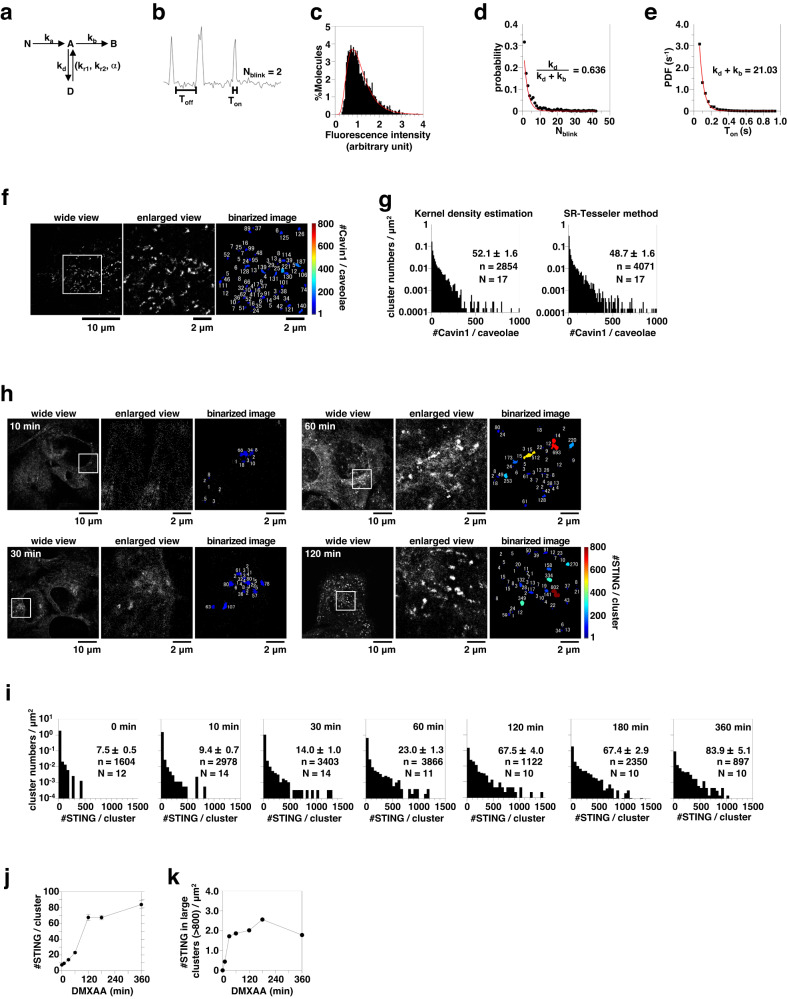
Fig. 1
Stimulation-dependent formation of STING cluster.
a Kinetic model of photoactivation and photobleaching of mEos4b. N, A, B, and D indicate nonactive, active, bleach, and dark states, respectively. k a , k b , k d indicate kinetic rates from N to A, f...
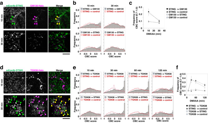
Fig. 2
The colocalization analysis of STING with the Golgi proteins.
a mEos4b-STING- and GM130-HaloTag7-expressing Sting -/- MEFs were stimulated with DMXAA for the indicated times. Typical PALM images of mEos4b-STING and dSTORM images of GM130-HaloTag7-SF650B. Colocal...
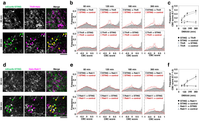
Fig. 3
The colocalization analysis of STING with recycling endosomal proteins.
a mEos4b-STING- and TfnR-HaloTag7-expressing Sting -/- MEFs were stimulated with DMXAA for the indicated times. Typical PALM images of mEos4b-STING and dSTORM images of TfnR-HaloTag7-SF650B. Colocaliz...
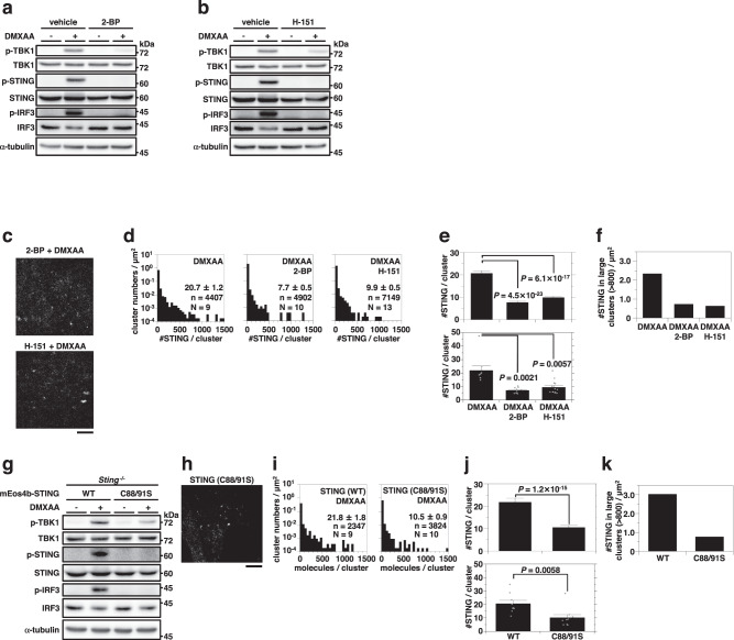
Fig. 4
Palmitoylation of STING is required for clustering.
mEos4b-STING-expressing Sting -/- MEFs were pretreated with ( a ) 2-bromopalmitate (2-BP) (200u2009u00b5M) for 4u2009h or ( b ) H-151 (10u2009u00b5M) for 2u2009h, and stimulated with DMXAA. Cell lysat...
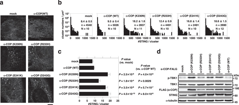
Fig. 5
Expression of the u03b1-COP variants induces the clustering of STING.
a Typical PALM images of Sting -/- MEFs expressing mEos4b-STING and/or u03b1-COP-FLAG (WT or the disease-causative variants). b The distribution of [#STING/cluster] in ( a ). The KDE method was used f...
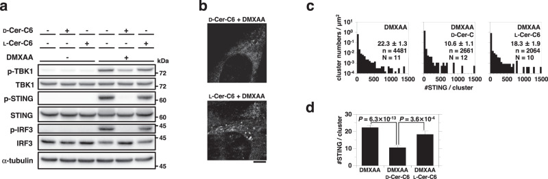
Fig. 6
Disturbing the Golgi lipid order with D-ceramide-C6 suppresses STING clustering.
a Sting -/- MEFs expressing mEos4b-STING were treated with D-ceramide-C6 (D-Cer-C6) (20u2009u03bcM) or L-ceramide-C6 (L-Cer-C6) (20u2009u03bcM) for 60u2009min. Cells were then stimulated with DMXAA fo...
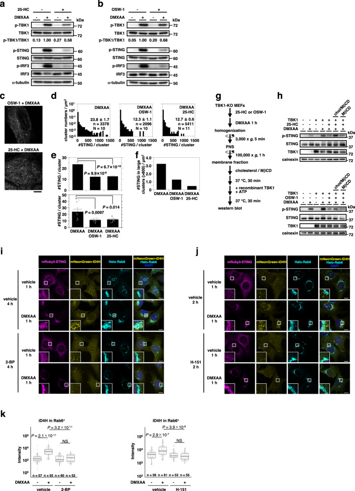
Fig. 7
Cholesterol in the TGN facilitates the clustering of STING.
Sting -/- MEFs expressing mEos4b-STING were pretreated with ( a ) 25-HC (30u2009u00b5M) for 16u2009h or ( b ) OSW-1 (0.125u2009nM) for 6u2009h, and stimulated with DMXAA for 60u2009min. Cell lysates w...
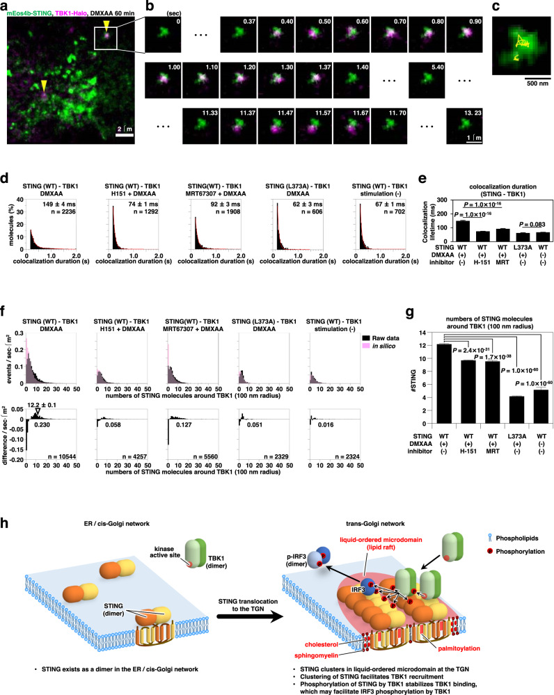
Fig. 8
The recruitment of TBK1 requires the clustering of STING.
mEos4b-STING and TBK1-HaloTag7 were stably expressed in STING/TBK1-double knockout MEFs. a A typical overlapped image obtained by simultaneous observation of mEos4b-STING clusters (green, PALM image) ...
Figure images are served from the NIH/NLM PubMed Central Open Access Subset or Europe PMC; copyright remains with the publishers and authors.
💬 Discussion
0 commentsNo comments yet. Be the first to start a discussion!
Leave a Comment