Abstract
Genetically encoded voltage indicators are emerging tools for monitoring voltage dynamics with cell-type specificity. However, current indicators enable a narrow range of applications due to poor performance under two-photon microscopy, a method of choice for deep-tissue recording. To improve indicators, we developed a multiparameter high-throughput platform to optimize voltage indicators for two-photon microscopy. Using this system, we identified JEDI-2P, an indicator that is faster, brighter, and more sensitive and photostable than its predecessors. We demonstrate that JEDI-2P can report light-evoked responses in axonal termini of Drosophila interneurons and the dendrites and somata of amacrine cells of isolated mouse retina. JEDI-2P can also optically record the voltage dynamics of individual cortical neurons in awake behaving mice for more than 30 min using both resonant-scanning and ULoVE random-access microscopy. Finally, ULoVE recording of JEDI-2P can robustly detect spikes at depths exceeding 400 μm and report voltage correlations in pairs of neurons.
🔬 Techniques
🔭 Microscopes
🧬 Organisms
💻 Software
✨ Fluorophores
🧪 Sample Preparation
🔬 Cell Lines
🏭 Microscope Brands
🧪 Reagent Suppliers
🔴 Lasers
📷 Detectors
🔎 Objectives
🎨 Filters
💻 Software Details
💾 Data Repositories
🏷️ Research Resource Identifiers (RRIDs)
Verified research resources used in this paper:
🏛️ Research Organizations (ROR)
Affiliated research institutions:
📋 Methods
Detailed methods are provided in the online version of this paper and include the following: RESOURCE AVAILABILITY Lead contact Further information and requests for resources and reagents should be directed to and will be fulfilled by the lead contact, Prof. François St-Pierre ( stpierre@bcm.edu or stpierre@alum.mit.edu ). Materials availability The JEDI-2P sequence is available from GenBank (GenBank: OL542830 ). All JEDI-2P plasmids, AAV packaging vectors, and the plasmid used to make the transgenic JEDI-2P flies are available from Addgene (see key resources table ).
Data and code availability
All data reported in this paper will be shared by the lead contact upon request. This paper does not report original code needed to reanalyze the data generated by this study. Any additional information required to reanalyze the data reported in this paper is available from the lead contact upon request.
EXPERIMENTAL MODEL AND SUBJECT DETAILS Cell lines
HEK293A and HEK293-Kir2.1 cell lines (sex: female in both cases) were used in this study. Detailed growth conditions varied with the experiment and are reported in the method details section. These cell lines were free of mycoplasma contamination and were authenticated by STR profiling by the Cytogenetics and Cell Authentication core (MD Anderson). Fly experiments All flies used for imaging were raised on standard molasses food at 25°C on a 12/12-h light-dark cycle. Female flies of the appropriate genotypes were collected on CO 2 within 1 day of eclosion and imaged at room temperature (20°C) 6–8 days after eclosion. The genotypes of the imaged flies in Figure 4 were: L2>>ASAP2f: +; UAS-ASAP2f/+; 21D-Gal4/+ L2>>JEDI-2P: yw/+; UAS-JEDI-2P/+; 21D-Gal4/+ The genotypes of the imaged flies in Figure S5 were: L2>>ASAP2f: +; UAS-ASAP2f/+; 21D-Gal4, jRGECO1b/+ L2>>ASAP3: w/+; UAS-ASAP3/+; 21D-Gal4, jRGECO1b/+ Retinal explants Retinal explants were extracted from healthy 2-month-old Chat - cre + female mice of strain B6;129S6- Chat tm2(cre)Lowl /J (RRID: IMSR_JAX:006410). Based on previous studies, we do not expect that gender would impact sensor expression or light responses in retinal explants. No previous procedures were performed prior to those described in the method details . Animals were group housed. Mice experiments with resonant scanning microscopy 3 males and 1 female mice from 2–6 months (at the time of imaging) were used for these experiments. Same sex littermates were housed together in individual cages with 1–4 mice per cage. Mice were maintained on a regular diurnal lighting cycle (12:12 light:dark) with ad libitum access to food and water and nesting material for environmental enrichment. Mice were housed in the Taub Mouse Facility of Baylor College of Medicine, accredited by AAALAC (The Association for Assessment and Accreditation of Laboratory Animal Care International). The animals used for this experiment were healthy and not involved in any previous procedures or experiments. Mice experiments with ULoVE microscopy 5 male wild-type C57BL/6J mice were housed in standard conditions (12-hour light/dark cycles, light on at 7 a.m., with water and food ad libitum ). No previous procedures were performed prior to those described in the method details . Mice were housed one per cage after surgery.
Show full methods section
Detailed methods are provided in the online version of this paper and include the following: RESOURCE AVAILABILITY Lead contact Further information and requests for resources and reagents should be directed to and will be fulfilled by the lead contact, Prof. François St-Pierre ( stpierre@bcm.edu or stpierre@alum.mit.edu ). Materials availability The JEDI-2P sequence is available from GenBank (GenBank: OL542830 ). All JEDI-2P plasmids, AAV packaging vectors, and the plasmid used to make the transgenic JEDI-2P flies are available from Addgene (see key resources table ).
Data and code availability
All data reported in this paper will be shared by the lead contact upon request. This paper does not report original code needed to reanalyze the data generated by this study. Any additional information required to reanalyze the data reported in this paper is available from the lead contact upon request.
EXPERIMENTAL MODEL AND SUBJECT DETAILS Cell lines
HEK293A and HEK293-Kir2.1 cell lines (sex: female in both cases) were used in this study. Detailed growth conditions varied with the experiment and are reported in the method details section. These cell lines were free of mycoplasma contamination and were authenticated by STR profiling by the Cytogenetics and Cell Authentication core (MD Anderson). Fly experiments All flies used for imaging were raised on standard molasses food at 25°C on a 12/12-h light-dark cycle. Female flies of the appropriate genotypes were collected on CO 2 within 1 day of eclosion and imaged at room temperature (20°C) 6–8 days after eclosion. The genotypes of the imaged flies in Figure 4 were: L2>>ASAP2f: +; UAS-ASAP2f/+; 21D-Gal4/+ L2>>JEDI-2P: yw/+; UAS-JEDI-2P/+; 21D-Gal4/+ The genotypes of the imaged flies in Figure S5 were: L2>>ASAP2f: +; UAS-ASAP2f/+; 21D-Gal4, jRGECO1b/+ L2>>ASAP3: w/+; UAS-ASAP3/+; 21D-Gal4, jRGECO1b/+ Retinal explants Retinal explants were extracted from healthy 2-month-old Chat - cre + female mice of strain B6;129S6- Chat tm2(cre)Lowl /J (RRID: IMSR_JAX:006410). Based on previous studies, we do not expect that gender would impact sensor expression or light responses in retinal explants. No previous procedures were performed prior to those described in the method details . Animals were group housed. Mice experiments with resonant scanning microscopy 3 males and 1 female mice from 2–6 months (at the time of imaging) were used for these experiments. Same sex littermates were housed together in individual cages with 1–4 mice per cage. Mice were maintained on a regular diurnal lighting cycle (12:12 light:dark) with ad libitum access to food and water and nesting material for environmental enrichment. Mice were housed in the Taub Mouse Facility of Baylor College of Medicine, accredited by AAALAC (The Association for Assessment and Accreditation of Laboratory Animal Care International). The animals used for this experiment were healthy and not involved in any previous procedures or experiments. Mice experiments with ULoVE microscopy 5 male wild-type C57BL/6J mice were housed in standard conditions (12-hour light/dark cycles, light on at 7 a.m., with water and food ad libitum ). No previous procedures were performed prior to those described in the method details . Mice were housed one per cage after surgery.
METHOD DETAILS Reagents for screening and in vitro benchmarking
Basic chemical reagents include: NaCl (S3014, Sigma-Aldrich), sucrose (S0389, Sigma-Aldrich), glucose (G8270, Sigma-Aldrich), HEPES (H3375, Sigma-Aldrich), KCl (P9541, Sigma-Aldrich), MgSO 4 (M2643, Sigma-Aldrich), K-gluconate (P1847, Sigma-Aldrich), EGTA (E3889, Sigma-Aldrich), MgCl 2 (M9272, Sigma-Aldrich), CaCl 2 (223506, Sigma-Aldrich), KOH (P250, Thermo Fisher) and NaOH (S5881, Sigma-Aldrich). Cell culture reagents include: high-glucose Dulbecco’s Modified Eagle Medium (D1145, Sigma-Aldrich), fetal bovine serum (F2442, Sigma-Aldrich), glutamine (G7513, Sigma-Aldrich), Penicillin/Streptomycin (P4333, Sigma-Aldrich), Geneticin (G418) Sulfate (30–234-CR, Corning), 30–70 kD poly-D-lysine (P7886, Sigma-Aldrich), 300 kD poly-D-lysine hydrobromide (P7405, Sigma-Aldrich) and phosphate-buffered saline (PBS, SH302560, HyClone, GE Healthcare). Primary neuronal culture reagents include: phenol-red-free Neurobasal medium (12348017, Gibco), B-27 (17504044, Gibco), Glutamax (35050061, Gibco) and cytosine β-D-arabinofuranoside (C1768, Sigma-Aldrich). Transfection and cloning reagents include: jetPRIME (114–15, Polyplus Transfection), FuGENE HD transfection reagent (E2311, Promega), lipofectamine 2000 (11668019, Thermo Fisher Scientific), FastDigest NheI (FD0974, Thermo Fisher Scientific) and FastDigest HindIII (FD0504, Thermo Fisher Scientific).
High-throughput GEVI screening
Plasmid construction Plasmids were assembled by standard molecular biology techniques and all cloned constructs were confirmed by Sanger sequencing (Eurofins Genomics LLC). GEVIs were cloned in pcDNA3.1/Puro-CAG vector. Unless noted otherwise, the reference protein cyOFP1 was fused to the C-terminus of GEVIs via a GSSGSSGSS linker ( van Rosmalen et al., 2017 ) ( Figure 1J ). ASAP1 and ASAP2s were subcloned from plasmids RRID: Addgene_52519 and RRID: Addgene_101274, respectively. ASAP3 was subcloned from a plasmid kindly provided by Dr. Michael Lin (Stanford). ASAP1-EGFP was cloned by replacing the circularly permuted GFP in ASAP1 (cpsfGFP-OPT) with EGFP (V2 – K239 ( Chamberland et al., 2017 )). Library construction Site-directed polymerase chain reaction (PCR) mutagenesis was used to construct saturation mutagenesis libraries, each targeting a single residue. Using single primers with the degenerate codon NNK results in the overrepresentation of some amino acids. To obtain a more uniform distribution of residues, we combined primers containing the NNT, VAA, ATG, or TGG codon (N = any base; V = A, G, or C) at a molar ratio of 16:3:1:1, respectively. The 20 μL PCR reaction mix contained 1 μL forward primer mix at 20 μM, 1 μL reverse primer at 20 μM, 50 ng template plasmid, and 10 μL 2× PCR master premix (PrimeSTAR HS DNA polymerase, Takara). DNA was amplified using the following protocol: an initial denaturation step at 98°C for 30 s; 35 amplification cycles of 98°C for 10 s, 57°C for 10 s, 72°C for 1 min/kb of fragment length; a final extension step at 72°C for 5 min. The pcDNA3.1/Puro-CAG backbone was linearized using the restriction enzymes NheI and HindIII. PCR products and linearized backbones were purified using gel electrophoresis and GeneJET Gel Extraction Kit (Thermo Fisher Scientific). PCR products were assembled in the vector backbone using the In-Fusion assembly system (In-fusion HD Cloning Plus, Takara) according to the manufacturer’s instructions. The In-Fusion reaction mix was transformed into commercial chemically competent bacteria (XL10-Gold, Agilent) with a transformation efficiency exceeding 5 × 10 9 CFU per μg DNA. Liquid cultures were inoculated with manually picked colonies, and purified plasmids were prepared using a 96-well plasmid purification kit (PureLink Pro, Thermo Fisher Scientific) following the manufacturer’s instructions.
Cell culture and transfection in 96-well plates
We used a modified HEK293 cell line that stably expressed human Kir2.1 channel ( Zhang et al., 2009 ) to maintain a resting membrane potential at approximately −77 mV in our conditions. HEK293-Kir2.1 cells were cultured at 37°C with 5% CO 2 in growth medium #1, which contained high-glucose Dulbecco’s Modified Eagle Medium supplemented with 10% fetal bovine serum (FBS), 2 mM glutamine, 100 unit/mL Penicillin, 100 μ/mL Streptomycin, and 750 μg/mL of the antibiotic G418 Sulfate (geneticin). G418 was added to maintain the expression of the Kir2.1 transgene, which was chromosomally integrated together with a G418 resistance gene. For screening GEVIs, glass-bottom 96-well plates (P96–1.5H-N, Cellvis) were first coated with 30–70 kD poly-D-lysine to promote cell adherence to the glass. Coating was done for 1 h at 37°C and plates washed twice with PBS. HEK293-Kir2.1 cells were then plated to 60–80% confluency in growth medium #2, which contained high-glucose Dulbecco’s Modified Eagle Medium supplemented with 5% FBS, 2 mM glutamine, 100 unit/mL Penicillin, and 100 μmg/mL Streptomycin. We generally selected 48 variants per library. According to a statistical model, our library generation and sampling strategy produced a ~91% theoretical probability that any given library included the best residue ( Nov, 2012 ). Each well was transfected according to the jetPRIME protocol: we used a mixture of 130 ng DNA, 0.4 μL jetPRIME transfection reagent, and 20 μL jetPRIME buffer in 150 μL of growth medium #2. Independent transfections were defined as transfections of separate wells in which DNA was added separately. Twenty-four hours post-transfection, 120 μL of the medium in each well was replaced with fresh growth medium #2 to minimize potential cytotoxicity from the transfection reagents. Forty-eight hours post-transfection the cells were washed twice with 200 μL of imaging solution (110 mM NaCl, 26 mM sucrose, 23 mM glucose, 5 mM HEPES, 5 mM KCl, 2.5 mM CaCl 2 , 1.3 mM MgSO 4 , adjusted to pH 7.4 with NaOH) at room temperature. Wells were filled with 100 μL of the imaging solution and screened with our 2PM high-throughput screening platform.
Two-photon screening system
An inverted microscope with multi-photon capability (A1R-MP, Nikon Instruments) was used for two-photon screening and in vitro characterization of GEVIs. The two-photon excitation light was generated by a titanium:sapphire femtosecond laser (Chameleon Ultra II, Coherent) with a repetition rate of 80 MHz and a tuning range between 680 nm and 1,080 nm. Laser power was tuned using an acousto-optic modulator and delivered to the sample plane through a 20× 0.75-NA objective (CFI Plan Apochromat Lambda, Nikon Instruments). The emission light from the sample was split using a 560-nm dichroic mirror and filtered by 525/50-nm (center wavelength/bandwidth) and 605/70-nm filters (Nikon Instruments) for green and red channels, respectively. Emitted photons were detected by gallium arsenide phosphide (GaAsP) photomultipliers tubes (PMTs). A motorized extended travel stage (H139E1, Prior) was used to control the position of the field of view and to hold 96-well plates and the electrophysiology perfusion chamber. To support automation of the system, data acquisition and output broads (PCI-6229 and PCI-6723, National Instruments) were connected to the microscope computer through a PXI Chassis (PXI-1033, National Instruments). The computer was equipped with 2 Intel Xeon E5–2630 v3 processors (total of 16 cores), 128 GB of DDR4 RAM, and four 2 TB SSDs in RAID 0 to facilitate high-speed imaging. JOBs scripts in NIS-Elements HC (version 4.60, Nikon Instruments) were used to control the microscope system (e.g., stage position), manage the optical configurations (e.g., excitations), initiate image acquisition, and trigger the stimulator. A digital isolated high-power stimulator (4100, A-M System) was used to provide electric field stimulation. Electric pulses were passed to a pair of electrodes made from 0.5 mm wide platinum wires (99.95% pure, AA10286BU, Fisher Scientific). The two L-shaped electrodes had a horizontal length of 2 mm and were 3 mm apart, and they were secured on a 3D-printed polylactic acid holder ( Figure 1F ). The holder was fixed to a motorized linear translation stage (MTS50-Z8, Thorlabs), which was used to move the electrodes in and out of individual wells. Two smaller manual linear translation stages (411–05S, Newport) were used to fine-tune the electrodes’ lateral position ( Figure 1E ). During stimulation, the electrodes were submerged under the imaging solution, about 350 μm above the bottom (i.e., 600 μm if calculated from the center of the electrode) ( Figures S1B and S1D ). The design was validated using 3D finite element modeling using Mathematica (Wolfram, Figure S1D ).
Two-photon GEVI screening Four non-overlapping fields of view
(FOV) of 512 × 32 pixels were imaged per well at 440 Hz using a resonant galvanometer scanner. The laser was set to 920 nm and tuned to 34–50 mW at the sample plane. The reference orange/red FP cyOFP1 was imaged first. 50 frames were captured so that noise could be reduced by averaging. Electric field stimulation was performed during continuous imaging of the green channel for 4000 frames or ~9 s. The stimulation protocol started with twenty monophasic square pulses with 1-ms width, 60-V amplitude, and an inter-pulse duration of 300-ms. This was followed by a 100-Hz train (10 monophasic square pulses with 2.5-ms width, 30-V amplitude, and an inter-pulse duration of 10 ms), although responses to this train were not used as a performance metric in the experiments described here.
Analysis of high-throughput screening data
Image analyses were performed by custom routines in MATLAB (version r2019b, MathWorks). Time-lapse images recorded in nd2 format were imported to MATLAB using the Bio-Formats toolbox (version 6.3.1) ( Linkert et al., 2010 ). For each channel (red and green) of each FOV, saturated pixels (e.g., from over-expressing cells) were removed and images were background corrected. An initial foreground mask was computed from the first 20 frames of each channel by applying pre-defined intensity thresholds to distinguish GEVI fluorescence from autofluorescence. The mask was applied to each image of the corresponding channel. The values of all pixels of an FOV were summated to obtain the overall change in fluorescence over time. We noticed that the quantification of response amplitudes could be distorted by overexpressing cells, bright extracellular fluorescent puncta, and intracellular aggregates due to slight impairment of GEVI plasma membrane targeting caused by the fused cyOFP. These problematic pixels were removed by discarding non-responsive pixels. To do this, we first corrected the green (GEVI) fluorescence obtained above for photobleaching. We performed a three-term exponential fitting on the mean fluorescence using data outside stimulation durations. The time constants were then used to estimate the trend for each pixel using the least-squares fitting. The trend of each pixel was removed using division. Correlation scores were then computed between the fluorescence of each foreground pixel and the overall FOV-level photobleaching-corrected fluorescence time course. The foreground pixels were then ordered by their correlation scores and binned in batches of 200 pixels. The foreground mask of responsive pixels was obtained by adding pixel bins of decreasing correlation scores until we maximized the signal-to-noise ratio. As done with the original threshold-based mask, all pixels were summated to obtain a single time course per FOV. To quantify photobleaching, this time course was normalized by the fluorescence at t = 0 and the area under the curve was quantified ( Figure 1K ). To measure responsivity, the unnormalized trace was corrected for photobleaching, using the same method motioned above, the responses to the 20 electrical field stimulations were averaged, and the peak response amplitude was quantified. GEVI brightness was calculated using the averaged fluorescence intensity of the first 20 frames in the green channel normalized by the average fluorescence intensity of the first 20 frames in the red channel. Normalization using the red channel was performed to correct for FOV-to-FOV differences in the number of transfected cells, the number of selected pixels, and overall expression (e.g., due to pipetting errors or biological variation). We developed compound metrics to simplify the ranking of indicators while considering multiple performance criteria. A theoretical framework suggested d ′ = R B τ O F F — where R is the response amplitude, B is the brightness, and τ OFF is the off-kinetics time constant — as a valuable metric to evaluate an indicator’s ability to detect isolated spikes ( Wilt et al., 2013 ). However, while slower off-kinetics increase the d ’, they also impair the identification of individual APs within a burst or fast spike train. We, therefore, decided to consider off-kinetics separately and defined the detectability index D l = R B by removing τ OFF from the d ’ equation. We also sought to consider the impact of photobleaching on voltage recording and avoid variants that are bright but bleach rapidly. We thus evaluated indicators based on both D I and photostability, and confirmed that three published ASAP variants could be distinguished using these metrics ( Figure 1L ). We also created a new metric — the detectability budget ( D B = R B ¯ = R B P ) — that combines all measured performance characteristics by replacing the initial brightness in the D I equation with the average brightness measured during the screening experiment.
ASAP2s in silico structure prediction
To build the ASAP2s structure ( Figures 1O and S2A ), the structures of the voltage-sensing and the cpGFP domains were first predicted using I-TASSER ( Yang et al., 2015 ) and SWISS-MODEL ( Waterhouse et al., 2018 ), respectively. The two domains were then fused in UCSF Chimera ( Pettersen et al., 2004 ). ModLoop ( Fiser and Sali, 2003 ) was used to optimize the interface between the voltage-sensing domain and the cpGFP. GEVI characterization in vitro Preparation for voltage clamp HEK293A cells (Thermo Fisher Scientific) were plated on 30–70 kD poly-D-lysine-coated circular cover glass (12 mm #0, 633009, Carolina) at 30% confluence in growth medium #2, two days before imaging. Chemical transfection was done on the same day of plating using 200 ng DNA and 0.6 μL FuGENE HD transfection reagent per well of a 24-well plate (P24–1.5H-N, Cellvis) following manufacturer’s instructions. The cells were cultured at 37°C with 5% CO 2 before and after transfection. Twenty-four hours post transfection, the transfection media was replaced with fresh growth medium #2 to minimize potential cytotoxicity from the transfection reagent. Glass micropipettes (TW150–4 or 1B150-F-4, World Precision Instruments) were prepared using a pipette puller (P-87 or P1000, Sutter) to achieve a tip resistance of 2–6 MΩ. Micropipettes were loaded with internal solution composed of 115 mM K-gluconate, 10 mM HEPES, 10 mM EGTA, 10 mM glucose, 8 mM KCl, 5 mM MgCl 2 , 1 mM CaCl 2 , adjusted to pH 7.4 with KOH. The micropipette was installed on a patch-clamp head-stage (CV-7B, Molecular Devices) and positioned by a micromanipulator (SMX series, Sensapex). The coverslip seeded with the transfected cells was placed in a custom glass-bottom chamber based on Chamlide EC (Live Cell Instrument) with glass bottom made with a 24 × 24 mm #1 coverslip, (D102424, Deltalab). Cells were continuously perfused with external solution (110 mM NaCl, 26 mM sucrose, 23 mM glucose, 5 mM HEPES, 5 mM KCl, 2.5 mM CaCl 2 , 1.3 mM MgSO 4 , titrated to pH 7.4 with NaOH, same as the imaging solution in High-throughput GEVI screening section) at ~4 mL/min with a peristaltic pump (505DU, Watson Marlow). Whole-cell voltage clamp was achieved using a MultiClamp 700B amplifier (Molecular Devices). Patch clamp data was recorded with an Axon Digidata 1550B1 Low Noise system with HumSilencer (Molecular Devices). Command voltage waveforms were compensated for the liquid junction potential. Recordings were considered satisfactory and were included in the final analysis only if the patched cell had an access resistance (Ra) smaller than 7 MΩ and a membrane resistance (Rm) larger than 10 times of Ra both before and after the recording. Voltage clamp under one-photon illumination GEVI characterization under 1PM was performed with the same microscope as for GEVI screening (above). Cells were illuminated with 470/24-nm light (SpectraX, Lumencor) and conditioned using the 477–503-nm band of a multi-band dichroic mirror (89100bs, Chroma). The irradiance at the sample plane was 4–8 mW/mm 2 . Green emitted photons were reflected towards the camera or PMT using the 503–542-nm band of the multi-pass dichroic (above) and filtered at 509–532 nm using a multi-pass filter (89101m, Chroma). Electrophysiological recordings were done at room temperature (~22°C), and cells were held at –70 mV, unless otherwise noted. Each patched cell expressing a GEVI variant was recorded using only one of the three voltage-clamp protocols. To predict GEVIs’ responses to action potentials (APs) under controlled conditions, we clamped HEK293 cells to follow a typical AP waveform and the resulting changes in GEVI fluorescence were monitored. The overall AP waveform had been recorded from a representative hippocampal neuron and was modified to have an amplitude of 100 mV and a full width at half maximum of 2 ms to mimic the shape of layer 2/3 cortical neurons at room temperature ( Hedrick and Waters, 2012 ). We performed experiments at room temperature because spikes are shorter at 37°C (0.7–0.8 ms, ( Hedrick and Waters, 2012 ; Kawaguchi, 1995 ; McCormick et al., 1985 )) and are thus suboptimally sampled with our imaging rate (1 kHz maximum under 1PM and 440 Hz under 2PM). Since GEVIs’ response time constants decrease with temperature at about the same rate as the decrease in spike width, GEVI responses are often tested at room temperature in vitro ( Chamberland et al., 2017 ; Kannan et al., 2018 ; Villette et al., 2019 ; Zou et al., 2014 ). Cells were stimulated with 5 AP waveforms at 2 Hz and 10 AP waveforms at 100 Hz. The excitation light was focused on the sample using a 20× NA-0.75 objective (CFI Plan Apochromat Lambda, Nikon Instruments). Time series recordings were captured at 1 kHz using the fast scan mode of a scientific complementary metal-oxide-semiconductor (sCMOS) camera (ORCA Flash 4.0 V2, Hamamatsu). Images were captured from a FOV with 2048 columns and 200 rows, which were binned by the camera after pixel readout, thus producing images of 512 × 50 pixels. To characterize fluorescence changes at or near steady state, cells were submitted to 1-s voltage steps to −100, −80, −60, −40, −20, 0, 20, 30, and 50 mV, with 1.5 s at the holding potential (−70 mV) between steps. Fluorescence was captured using the same optical configuration and imaging protocol as in the previous paragraph. Traces (e.g., in Figure 2A ) were smoothed by a 24-ms moving average. To evaluate the sensors’ kinetics, we conducted three 1-s 100-mV depolarization pulses from −70 to 30 mV. Between each pulse, cells were held at −70 mV for 1.4 s. Recordings were performed at 21–23°C (room temperature) or 32–35°C (closer to the 37°C temperature of mice brains) using a feedback-controlled inline heater system (inline heater SH-27B, controller TC-324C, cable with thermistor TA-29, Warner instruments) to maintain the temperature in the perfusion chamber. A diaphragm was used to reduce the diameter of the excitation spot so that during imaging only one cell at the center of the FOV was illuminated. To maximize photon collection, we used an objective with higher numerical aperture (NA) than above (40× NA-0.95, CFI Plan Fluor oil immersion, Nikon Instruments). To capture fluorescence changes at higher temporal resolution than achievable with our camera, a multialkali photomultiplier tube (PMT, PMM02, Thorlabs) was installed on one of the side ports of the microscope. A LabVIEW (version NXG 5.0, National Instruments) routine was used to control the PMT bias voltage and record the output voltage using the data acquisition and output boards. Data were collected at 80 kHz. The output voltage from the PMT was analyzed by a custom routine written in MATLAB to obtain fluorescence signal for each cell. The raw data was first downsampled to 20 kHz. Then, photobleaching correction was done by performing a three-term exponential fitting on the baseline (when the cell was held at −70 mV) and removing the trend from the entire signal using division. The corrected signal was cropped from 0.1-s before the estimated depolarization or the repolarization onset to 1-s after the estimated depolarization or repolarization onset. The exact onset timing was fitted together with other coefficients with either single-exponential (F(t) = c + (k × exp((t - t 0 ) × λ)) × (t > t 0 ) + k × (t ≤ t0)) or dual-exponential (F(t) = c + (k × exp((t - t 0 ) × λ) + k 2 × exp((t - t 0 ) × λ 2 )) × (t > t 0 ) + (k + k 2 ) × (t ≤ t 0 )) model where the t is the independent variable, F is the dependent variable, and the rest are the coefficients to be fitted. Among these coefficients, c describes the mean plateau fluorescence, k or k 2 describe the relative ratio of each exponential component, λ or λ 2 describe (minus) inverse of the time constant(s), and t 0 is an offset indicating the exact event onset timing. Voltage clamp under two-photon illumination To evaluate sensors’ performance under 2PM, we used one integrated protocol to characterize the fluorescence changes in response to AP waveforms and step voltages at ~22°C. The same AP waveforms that were used under 1PM were used under 2PM, and each cell was stimulated with 20 AP waveforms at 2 Hz and 10 AP waveforms at 100 Hz, and then held for 1 s at −100, −80, −60, −40, −20, 0, 20, 30, and 50 mV from a holding potential of −70 mV. AP waveforms were as described above (1PM characterization). We used a R ≥ 2-s interval before the AP waveform assay and the voltage steps and 1.5-s intervals between each voltage step. These intervals ensured that GEVI fluorescence had returned to its resting state. Cells were imaged using the same inverted microscope as 2P screening, under 40× magnification (NA-0.95, CFI Plan Fluor oil immersion, Nikon Instruments). The resonant galvanometer scanner was used to direct the 920-nm excitation laser at 15% of the full power or 31 mW at the sample plane with the detector photomultiplier tubes’ gain set to 20. Videos were taken with a resolution of 512 × 32 pixels and a frame rate of 440 Hz.
Two-photon excitation spectra
To determine the two-photon excitation spectrum for JEDI-2P, we cloned JEDI-2P, ASAP2s and EGFP in pcDNA3.1/Puro-CAG plasmid between the NheI and HindIII sites with no reference protein attached. ASAP2s and EGFP were used as controls in this experiment. These constructs were then transfected into HEK293-Kir2.1 cells using jetPRIME. The cells were plated in wells of a 24-well plate (P24–1.5H-N, Cellvis) coated with 30–70 kD poly-D-lysine. Each well was transfected according to the jetPRIME protocol with a mixture of 650 ng DNA, 1.8 μL jetPRIME transfection reagent, and 65 μL jetPRIME buffer in 500 μL of culture medium. Independent transfections were defined as transfections of separate wells in which DNA was added separately. Four hours after transfection, the transfection media was replaced with fresh growth medium #2 to minimize the potential cytotoxicity from transfection reagents. Two days after transfection, cells were washed with and imaged in external solution (see GEVI characterization in vitro ). Images were acquired using the same microscope as used for screening (see Two-photon screening system ) using a 20× NA-0.75 objective (CFI Plan Apochromat Lambda, Nikon). Laser pulses were not pre-compensated for dispersion in the microscope optical path. Excitation wavelengths from 700 to 1080 nm were used in 10-nm increments. At each wavelength, the laser was tuned to a power of 10–20 mW at the sample plane, as measured by a microscope slide power sensor (S170C or S175C, Thorlabs). Each FOV was scanned at all wavelengths by two galvanometer optical scanners with a pixel dwell time of 12.1 μs. Fluorescence values were corrected by subtracting the background. Small deviations in the actual power from the target power were corrected by assuming a quadratic dependence of fluorescence on illumination power at the sample plane. Power was kept unchanged for all fluorophores. Because there is no significant difference in the fluorescence at 920 nm acquired before and after the spectral scan, photobleaching correction was not needed and was not performed. One-photon excitation and emission spectra To determine the one-photon excitation and emission spectra for JEDI-2P, we first constructed the pcDNA3.1/Puro-CAG-EGFP-CAAX plasmid as a control by subcloning the CAAX membrane anchoring motif ( Choy et al., 1999 ) to the C-terminal of EGFP. CAAX motif was added to achieve membrane localization like JEDI-2P. HEK293-Kir2.1 cells were plated on wells of a 6-well plate (3516, Corning) to reach a confluency of 60–80% on the day of transfection. Three micrograms of pcDNA3.1/Puro-CAG plasmids expressing JEDI-2P or EGFP-CAAX were transiently transfected using 9 μL jetPRIME transfection reagent, and 200 μL jetPRIME buffer per well. The transfection medium was replaced after 4 h with fresh growth medium #2 to minimize potential cytotoxicity from the transfection reagent. Forty-eight hours after transfection and for each fluorophore, cells from two wells were detached, washed twice and diluted into in the same imaging solution used for 2PM screening, and pooled into a single well of a 96-well plate (P96–1.5H-N, Cellvis). Pooling the cells to a dense preparation was important to produce a strong signal that could be robustly detected by the plate reader. Untransfected cells were also prepared to determine the background autofluorescence levels. A hemocytometer was used to plate a similar number of cells between conditions. Spectra were determined by using a plate reader (Cytation 5, BioTek) to quantify fluorescence from wells of the 96-well plates prepared above. Excitation spectra were acquired by scanning excitation wavelengths from 350 to 535 nm in increments of 1 nm and a bandwidth of 10 nm and collecting emission intensity at 560/10 nm. Emission spectra were acquired by exciting at 430/10 nm and measuring emitted photons from 460 to 650 nm in increments of 1 nm and with a bandwidth of 10 nm. Individual scans of excitation and emission spectra were corrected for autofluorescence by subtracting the values from untransfected cells at each wavelength, and then normalized to their respective peaks. The final excitation and emission spectra were determined by averaging the normalized spectra for each of the constructs. The peaks were determined by averaging the peaks from each individual scan. GEVI one-photon photostability To determine the one-photon photostability for JEDI-2P, we used the same vectors used for 2PM screening, i.e, pcDNA3.1/Puro-CAG expressing JEDI-2P/ASAP2s/ASAP3/ASAP1-N124V-R406K/ASAP2s-T207H with cyOFP1 attached to the C-terminal of the GEVIs through a GSSGSSGSS linker. These plasmids were transfected into HEK293-Kir2.1 cells in 96-well format using the same methods as described in the Cell culture and transfection in 96-well plates section. Twenty-four hours after transfection, 120 μL of the transfection media in each well was replaced with fresh growth medium #2 to minimize the potential cytotoxicity from transfection reagents. Two days after transfection, cells were washed twice and imaged in the same imaging solution used for 2PM screening. Images were acquired using the same microscope as used for screening (see Two-photon screening system ) using a 20× NA-0.75 objective (CFI Plan Apochromat Lambda, Nikon). For each FOV, one image for the cyOFP1 was taken first, followed by a time-lapse video for the GEVIs. The cyOFP1 image, i.e. the reference channel, was illuminated with 555/15-nm light (SpectraX, Lumencor) and conditioned using the 542–571-nm band of a multiband dichroic mirror (89100bs, Chroma), which has an irradiance of 18 mW/mm 2 at the sample plane. The GEVI video, i.e. the target channel, was illuminated with 470/24-nm light (SpectraX, Lumencor) and conditioned using a long-pass dichroic mirror (T495lpxr, Chroma), which has an irradiance of 15 mW/mm 2 at the sample plane. The emission light from the target channel was further filtered with a band-pass filter (ET525/50, Chroma) to minimize the bleed-through from cyOFP1 emission. Both channels were captured with 5-ms exposure time per frame using an sCMOS camera (ORCA Flash 4.0 V2, Hamamatsu). The target channel was sampled at 2 Hz for the first 20 frames (9.5-sec), and 1 Hz for another 180 (3 mins, Figure 1C ) or 300 frames (5 mins, Figures S4G and S4H ). Photobleaching traces were calculated from the foreground pixels selected by applying a brightness threshold on both background-corrected channels. The photostability of the sensors was quantified as the area-under-the-curve of the photobleaching trace normalized by the fluorescence at t = 0. The brightness of the sensors was quantified as the green channel fluorescence of the first frame in the video divided by the red channel fluorescence. For each of the GEVI, 6 ( Figure 1C ) or 4 ( Figures S4G and S4H ) wells of replicates were tested with n = 1 ( Figure 1C ) or 2 ( Figures S4G and S4H ) FOVs in each of the wells. Analysis was performed per FOV and averaged for each well, and the final statistics were drawn at the well level.
Confocal imaging of GEVIs in dissociated neurons
Primary rat cortical neurons were isolated from day 18 Long-Evans rat embryos. Cortices were dissected, dissociated with papain (Worthington Biochemical Corporation), washed with trypsin inhibitor (Sigma), and seeded at 5:0×10 5 cells/mL on 12 mm No. 0 coverslips (633009, Carolina Scientific), each placed in one well of a 24-well plate (3524, Corning). Each well was filled with 500 μL of Neurobasal medium (Invitrogen) supplemented with B-27 (Invitrogen), 2 mM Glutamax (Gibco), 10% FBS, 100 unit/mL Penicillin, and 100 μg/mL Streptomycin. The coverslips were pre-coated with 300 kD poly-D-lysine hydrobromide and washed twice with PBS before seeding. The plating day was considered as day in vitro (DIV) 0. The next day, 90% of the media was replaced with a culturing medium consisted of phenol-free Neurobasal medium (Gibco), B-27 (Gibco), 2 mM Glutamax (Gibco), 100 unit/mL Penicillin, and 100 μg/mL Streptomycin. Half of the media was henceforth replaced with fresh culturing medium every 3–4 days. Around DIV 6, further glia growth was limited by adding cytosine β-D-arabinofuranoside to the culturing media to a final concentration of 2 μM. All media were pre-equilibrated for at least 24 h at 37°C in air with 5% CO 2 before usage. A neuronal expression vector was constructed by cloning JEDI-2P under the control of the neuron-specific hSyn promoter by replacing ASAP2s in pAAV-hSyn-ASAP2s (RRID: Addgene_101276) with JEDI-2P. mCherry was cloned into pcDNA3.1/Puro-CAG vector between the NheI and HindIII sites as a soluble marker of neuronal transfection. Neurons were transfected at DIV 9 using 1 μL lipofectamine 2000 and 800 ng total DNA, including 100 ng pAAV-hSyn-JEDI-2P, 50 ng pcDNA3.1/Puro-CAG-mCherry, and 650 ng pNCS bacterial expression vector as buffer/filler DNA. Laser-scanning confocal images were obtained 3 days after transfection using a high-speed confocal microscope (LSM880 with Airyscan, Zeiss) driven by the Zen software (version 2.3 SP1, Zeiss). The microscope was equipped with a 40× 1.1-NA water immersion objective (LD C-Apochromat Korr M27, Zeiss), a 488-nm argon laser (LGK7812, Lasos) set to 20% power (~200 μW) and a per-pixel dwell time of 2 μs. Emission light was filtered using a multipass beamsplitter (MBS 488/561/633, Zeiss) and acquired with a 32 channel GaAsP detector (Airyscan, Zeiss) with a detector gain of 850, and a 1.28-Airy unit pinhole size. To increase the signal-to-noise ratio, 2 scans were performed and averaged for each image. Airyscan processing was applied to the images to increase the resolution. Z stacks were made with 0.27 μm between images. Figure 2K corresponds to a maximum intensity projection from Z stack with 26 images. mCherry was not captured in the final image. 2P voltage imaging in isolated mouse retina Virus construction and packaging JEDI-2P was cloned into the pAAV vector (RRID: Addgene_20298) by replacing the hChR2(H134R)-EYFP sequence with JEDI-2P with In-Fusion method. The double-floxed inversed JEDI-2P under the control of EF-1α promoter was then packaged into Adeno-Associated Viruses serotype 1 (AAV2/1) at BCM Neuroconnectivity Core. The final AAV, referred below as AAV2/1-EF1α-DIO-JEDI-2P, had a final concentration of 3–4×10 12 GC/mL.
Surgeries and GEVI expression
All animal procedures were approved by the governmental review board (Regierungspräsidium Tübingen, Baden-Württemberg, Konrad-Adenauer-Str. 20, 72072 Tübingen, Germany) and performed according to the laws governing animal experimentation issued by the German Government. To express JEDI in starburst amacrine cells (SACs), we injected 1 μL of the viral construct AAV2/1-EF1α-DIO-JEDI-2P into the vitreous humor of each eye of anaesthetized 5-week-old ChAT Cre mice (n = 2, RRID: IMSR_JAX:006410, The Jackson Laboratory) as described recently ( Franke et al., 2017 ). Imaging experiments were performed 4 weeks after injections. In brief, the retina was dissected from the eyecup, flat-mounted on a filter paper and moved to the recording chamber of the microscope.
Two-photon imaging
For visual stimulation, we used a DLP-based projector ( Franke et al., 2019 ) with UV (390 nm) and green (576 nm) LEDs displaying either 1-s local light flashes (100 μm diameter) or a local chirp stimulus (74 μm diameter, 63 μm offset from the scan field center; for details on chirp stimulus, see ( Baden et al., 2016 ). All visual stimuli were displayed using both UV and green LED, corresponding to an achromatic stimulus. To record light-evoked responses from SACs, we used a movable objective microscope (MOM)-type two-photon microscope ( Euler et al., 2009 ) and acquired time-lapsed 128×1 (at 1.04 kHz), 128×4 (at 260.4 Hz) or 64×32 (at 15.6 Hz) scans for somatic and dendritic voltage imaging with the laser tuned to 927 nm at 9–12 mW laser intensity. The visual stimulus was presented during the retrace period of the laser scanning to prevent light artifacts in the imaging ( Franke et al., 2019 ). The retrace period was ~20% of the scan duration (e.g., 0.2 ms for a 1-ms line scan). The microscope setup was equipped with GaAsP photomultiplier tubes and a bandpass emission filter (HQ 510/84, AHF/Chroma).
Experimental design
Our experiments were replicated across fields of view and mice. Replicate numbers and definitions are listed in the Figure legends. As there were no comparisons, sample size estimation and blinding in data collection and analysis do not apply. Fields of view were excluded from analysis if the retina was not expressing the sensor or if there were no detectable changes in fluorescence in response to light stimulation.
Data analysis
Pixels of individual imaging scans were chosen for further analysis by measuring their standard deviation (SD) over time. The pixels with the 30% highest SD were analyzed. The voltage trace for each pixel was extracted. Changes in the baseline were corrected by high-pass filtering above 0.2 Hz for frame scans or 0.5 Hz for line scans. Traces were then mean-subtracted and normalized to the standard deviation for that pixel. For trial averaging, traces were aligned relative to trial onset and then resampled to 40 Hz for step and chirp responses. For the 64×32 (15.6 Hz) scans, resampling at higher temporal resolution than the original framerate is possible because the stimulus was presented at different times relative to the recordings for each trial. For SAC somata, selected pixels were split into individual soma by eye. Then, traces of all selected pixels in a field (or soma) were averaged into one region-of-interest (ROI) and filtered with a Savitzky-Golay filter (window of 125 ms and a polynomial order of 2) to remove high frequency noise. Finally, for each ROI we computed the mean activity across stimulus repetitions (n = 20 for flashes,n = 10 for chirp stimuli). To evaluate JEDI-2P photostability, we standardized pixel selection by analyzing the same number (38) of responsive pixels per field of view. Voltage imaging in Drosophila visual neurons using galvanometric point-scanning 2PM Fly husbandry, in vivo two-photon imaging of flies, visual stimulation, and data analysis were done as previously described ( Chamberland et al., 2017 ; Yang et al., 2016 ) and as described below. Transgenic flies JEDI-2P and ASAP3 were cloned into the pJFRC7–20XUAS vector ( Pfeiffer et al., 2010 ) using standard molecular cloning methods, with XbaI and XhoI as the restriction sites (GenScript Biotech for JEDI-2P). The UAS-JEDI-2P and UAS-ASAP3 transgenes were each inserted into the attP40 phiC31 landing site by injection of fertilized embryos (BestGene for JEDI-2P, Rainbow Transgenic for ASAP3). UAS-JEDI-2P was additionally inserted into the VK00005 phiC31 landing site though all experiments presented here used the attP40 insertion. The L2 Gal4 driver (21D-Gal4) was from Rister et al. (2007) . The genotypes of the imaged flies in Figure 4 were: L2>>ASAP2f: +; UAS-ASAP2f/+; 21D-Gal4/+ L2>>JEDI-2P: yw/+; UAS-JEDI-2P/+; 21D-Gal4/+ The genotypes of the imaged flies in Figure S5 were: L2>>ASAP2f: +; UAS-ASAP2f/+; 21D-Gal4, jRGECO1b/+ L2>>ASAP3: w/+; UAS-ASAP3/+; 21D-Gal4, jRGECO1b/+ Fly husbandry All flies used for imaging were raised on standard molasses food at 25°C on a 12/12-h light-dark cycle. Female flies of the appropriate genotypes were collected on CO 2 within 1 day of eclosion and imaged at room temperature (20°C) 6–8 days after eclosion.
Fly surgery
Flies were cold anaesthetized, positioned in a fly-shaped hole cut in steel foil such that their heads were tilted forward approximately 90° to expose the back of the head capsule above the foil while leaving most of the retina below the foil, and then affixed in place with UV-cured glue (NOA 68T from Norland Products Inc.). The brain was exposed by removing the overlying cuticle and fat bodies with fine forceps, and an oxygenated saline-sugar solution ( Wilson et al., 2004 ) was perfused over the fly. The saline composition was as follows: 103 mM NaCl, 3 mM KCl, 5 mM TES, 1 mM NaH 2 PO 4 , 4 mM MgCl 2 , 1.5 mM CaCl 2 , 10 mM trehalose, 10 mM glucose, 7 mM sucrose, and 26 mM NaHCO 3 . The pH of the saline equilibrated near 7.3 when bubbled with 95% O 2 /5% CO 2 .
Two-photon imaging
Neurons were imaged with a Leica TCS SP5 II two-photon microscope with a 20×/1.0-NA water immersion objective (Leica HCX APO) and a pre-compensated femtosecond laser (Chameleon Vision II, Coherent). The excitation wavelength was 920 nm and 5–20 mW of power was applied to the sample. Emitted photons were filtered by a 525/50-nm filter and collected with a Hybrid Detector (HyD, Leica). The data were acquired at a constant frame rate of 82.4 Hz using a frame size of 200×20 pixels, 15× digital zoom, a line scan rate of 1,400 Hz, and bidirectional scanning. L2 cells were imaged at their arbor in medulla layer M2. Total imaging time per fly never exceeded 1 h.
Visual stimulation
Visual stimuli were generated with custom-written software using MATLAB (MathWorks) and presented using only the blue LED of a projector (DLP Lightcrafter 4500, Texas Instruments) in Pattern Sequence mode. The stimulus was refreshed at 300 Hz and utilized 6 bits/pixel, allowing for 64 distinct luminance values. The stimulus was projected directly onto a 9 cm × 9 cm rear-projection screen positioned approximately 8 cm anterior to the fly that spanned approximately 70° horizontally and 40° vertically of the fly’s visual field. A small square of the stimulus was also simultaneously projected onto a photodiode (SM05PD1A, Thorlabs) configured in a reversed-biased circuit. The stimulus was filtered with a 482/18-nm bandpass filter so that it could not be detected by the microscope detectors. The radiance at 482 nm was approximately 78 mW sr −1 m −2 . The imaging and the visual stimulus presentation were synchronized using triggering functions provided by the LAS AF Live Data Mode software (Leica) as well as the signal from the photodiode directly capturing projector output. A data acquisition device (NI DAQ USB-6211, National Instruments) connected to the computer was used to acquire the photodiode signal, generate a trigger signal at the beginning of stimulus presentation, and acquire the trigger produced by the LAS software at the start of each imaging frame. This allowed the imaging and the stimulus presentation to initialize in a coordinated manner and ensured that stimulus presentation details were saved together with imaging frame timings (in MATLAB .mat files) to be used in subsequent processing. Data was acquired at 5 kHz. The visual stimuli used were: 300-ms search stimulus: alternating full contrast light and dark flashes, each 300 ms in duration, were presented at the center of the otherwise dark screen. The stimulus was such that from the perspective of the fly, the flashing region was 8° from each edge of the screen. In subsequent analysis, the responses to this stimulus were used to select regions of interest (ROIs) with receptive fields located at the center of the screen instead of at the edges. This stimulus was presented for 5,000 imaging frames (61 s) per field of view. 20-ms light and dark flashes from gray ( Figures 4C and 4D ): single 20-ms light and dark flashes, with 500-ms of gray between the flashes, were presented over the entire screen. The light and dark flashes were randomly chosen at each presentation. The Weber contrast of the flashes relative to the gray was 1. This stimulus was presented for 10,000 imaging frames (122 s) per field of view. 300-ms full-field flash ( Figure 4F ): alternating full contrast light and dark flashes, each 300 ms in duration, were presented over the entire screen. This stimulus was presented for 100,000 imaging frames (20.3 mins) per field of view.
Experimental design
Our experiments were replicated across many cells and flies. Replicate numbers and definitions are listed in the Figure legends. Data collection and analysis were not done blinded. However, the data was analyzed using automated procedures applied identically for all datasets. Exclusion criteria for flies and regions-of-interest (ROIs) are described below. We estimated the sample size needed based on our previous work with similar assays.
Data analysis
The acquired time series were saved as .lif files and read into MATLAB using Bio-Formats (Open Microscopy Environment) ( Linkert et al., 2010 ). Raw images in each time series were aligned in x and y coordinates by maximizing the cross-correlation in Fourier space of each image with a reference image (the average of the first 30 images in the time series). For each time series, ROIs around individual arbors were selected by thresholding the series-averaged image with a value that generates appropriate ROIs, and then splitting any thresholded ROIs consisting of merged cells and/or drawing any additional ROIs that were missed by the thresholding. For each imaging frame within the time series, intensity values for the pixels within each ROI were averaged and the mean background value (the average intensity in a region of the image without cells) was subtracted. To correct for photobleaching, the time series for each ROI was fit with the sum of two exponentials, and in the calculation of ΔF/F 0 = (F(t) − F 0 )/F 0 , the fitted value at each time t was used as F 0 . This is mathematically equivalent to calculating ΔF/F 0 from the trace obtained by dividing F(t) by the photobleaching fitted function. For the 300-ms full-field flash and the 300-ms search stimuli, all frames were used to compute the fit, thereby placing ΔF/F 0 = 0 at the mean response after correction for bleaching. For the 20-ms light and dark flashes from gray stimuli, only frames that fell in the last 25% of the gray period were used to fit the bleaching curve; this places ΔF/F 0 = 0 at the mean baseline the cell returns to after responding to the flash instead of at the mean of the entire trace. We did not place the ΔF/F 0 = 0 at the mean baseline of the entire trace because responses to the light and dark flashes are not necessarily equal and opposite. Time series with uncorrected movement, which was apparent as irregular spikes or steps in the ΔF/F 0 traces that were coordinated across ROIs, were discarded. For the 300-ms full field flash, the 300-ms search, and the 20-ms light and dark flashes from gray stimuli, the stimulus-locked average response was computed for each ROI by reassigning the timing of each imaging frame to be relative to the stimulus transitions (dark to light or light to dark for the 300-ms full-field flash or search stimuli, gray to light or gray to dark for the light and dark flashes from gray) and then computing a simple moving average. The averaging window was 8.33 ms and the shift was 8.33 ms, which effectively resampled our data from 82.4 Hz to 120 Hz. As the screen on which the stimulus was presented did not span the fly’s entire visual field, only a subset of imaged ROIs experienced the stimulus across approximately the entire extent of their spatial receptive fields. These ROIs were identified based on having a response of the appropriate sign to the 300-ms search stimulus. ROIs lacking a response to these stimuli or having one of the opposite signs were not considered further. The quantification metrics for each ROI ( Figure 4D ) were computed as follows: The peak response to each flash was the ΔF/F 0 value farthest from zero in the expected direction of the initial response (depolarization or hyperpolarization). The time to peak was the time at which this peak response occurred, relative to the start of the light or dark flash. Voltage imaging in the mouse cortex using resonant scanning 2PM All procedures were carried out in accordance with the ethical guidelines of the National Institutes of Health and were approved by the Institutional Animal Care and Use Committee (IACUC) of Baylor College of Medicine.
Viral construction and packaging
We created a soma-targeted version of JEDI-2P, which we abbreviate as JEDI-2P-Kv in the construct names below. JEDI-2P-Kv was cloned into the pAAV vector (RRID: Addgene_20298) by replacing the hChR2(H134R)-EYFP sequence with JEDI-2P-GSSGSSGSS-Kv with In-Fusion method, where Kv is the C-terminal motif of Kv2.1 potassium channel for soma localization ( Lim et al., 2000 ). The double-floxed inversed JEDI-2P-Kv under the control of EF1α promoter was then packaged into Adeno-Associated Viruses serotype 1 (AAV2/1) at the Canadian Neurophotonics Platform (Université Laval) viral vector core. The final AAV, referred below as AAV2/1-EF1α-DIO-JEDI-2P-Kv, had a final concentration of around 7.5×10 12 GC/mL. In the corresponding main text section and figures, to avoid using an additional abbreviated construct name (JEDI-2P-Kv), we simply state that we used the soma-localized version of JEDI-2P.
Viral injections
Functional imaging was performed in B6;129S-Slc17a7/J mice (RRID: IMSR_JAX:023527) injected with AAV2/1-EF1α-DIO-JEDI-2P-Kv resulting in JEDI-2P expression in pyramidal cells. Injections were performed through a burr hole targeted stereotactically to visual cortex (2.8 mm lateral of the midline, and 1.5 mm anterior to the lambdoid suture). In each mouse, 500–1000 nL of virus was injected approximately 350 μm deep via a nano-injection pump (WPI). After at least 2 weeks to allow for expression, mice craniotomies were performed above the injection site, and mice were prepared each with a cranial window as described below. Mice were housed in standard conditions (12-h light/dark cycles, light on at 6 a.m., with water and food ad libitum ). Cranial window Anesthesia was induced with 3% isoflurane and maintained with 1.5% to 2% isoflurane during the surgical procedure. Mice were injected with 5–10 mg/kg ketoprofen subcutaneously at the start of the surgery for analgesia. Anesthetized mice were placed in a stereotaxic head holder (Kopf Instruments) and their body temperature was maintained at 37°C throughout the surgery using a homeothermic blanket system (Harvard Instruments). After shaving the scalp, bupivacaine (0.05 cc, 0.5%, Marcaine) was applied subcutaneously, and after 10–20 min an approximately 1-cm 2 area of skin was removed above the skull and the underlying fascia was scraped and removed. The wound margins were sealed with a thin layer of surgical glue (VetBond, 3M), and a 13-mm stainless-steel washer clamped in the headbar was attached with dental cement (Dentsply Grip Cement). At this point, the mouse was removed from the stereotaxic frame and the skull was held stationary on a small platform by means of the newly attached headbar. Using a surgical drill and long straight shank (HP) 1/2 burr, a 4-mm craniotomy was made centered on the viral injection burr hole, and the exposed cortex was washed with artificial cerebrospinal fluid (ACSF) (125 mM NaCl, 5 mM KCl, 10 mM Glucose, 10 mM HEPES, 2 mM CaCl 2 , 2 mM MgSO 4 ). The cortical window was then sealed with a 4-mm diameter coverslip (Warner Instruments), using cyanoacrylate glue (VetBond). Resonant scan 2P voltage imaging Two-photon (2P) imaging was performed on a Thorlabs Bergamo resonant scanning microscope with 920 nm excitation via a titanium:sapphire femtosecond laser (Chameleon Vision II, Coherent). A 1.1-NA 25× objective lens was used (CFI75 Apochromat 25XC W, Nikon Instruments) except for patching, where a 0.8-NA long-working distance 16× lens (CFI75 LWD 16X W, Nikon Instruments) was used to allow space for the patch pipette to approach the tissue under the microscope. The emission was split by a dichroic mirror into two channels: the green channel used a 525/50 nm filter, and the red channel used a 625/90 nm filter, before being collected by two photomultiplier tubes.
ScanImage software
(Vidrio) was used to control the microscope and acquire imaging data. Imaging power was kept between 20–70 mW depending on depth and field of view. In-vivo patching To perform simultaneous 2P imaging and patching, the coverslip was removed and replaced with a new coverslip that had been predrilled with a small (~500 μm diameter) hole using a diamond-tipped burr (Choltene/Whaledent). The opening in the coverslip was positioned so that a patch pipette approaching at an angle through the hole could target nearby JEDI-2P-expressing cells. Mice were kept under 1–2% isoflurane anesthesia throughout the experiment and their temperature was maintained with a homeothermic blanket. Patch pipettes were pulled from borosilicate glass (1.5 mm outer diameter × 0.86 mm inner diameter, Sutter Instruments) to an impedance of 6–12 MΩ. Pipettes were filled with standard external solution (ACSF) and Alexa Fluor 594 dye was added (50 μM) to allow visualization of the pipette and extracellular space ( Häusser and Margrie, 2014 ). A manometer (Fisher Scientific 06–664-19) and custom-built pressure manifold allowed fast switching between high pressures while entering the bath and penetrating the dura (~150 mbar), and low pressures (~20–50 mbar) while advancing the pipette through the cortex under 2P guidance, which helped to reduce the overall volume of intracellular solution ejected from the pipette. Bias currents were zeroed once the pipette was placed in the bath. JEDI-2P-expressing cells were targeted for recording by approaching the cell under 2P guidance and establishing a juxtacellular seal that enabled visualization of neuronal spiking. After each recording, positive pressure was applied, which often broke open the cell membrane and enabled intracellular injection of the Alexa Fluor 594 dye that enabled us to confirm that we were recording from the cell that we had been imaging. Voltage imaging without in-vivo patching Voltage imaging experiments without in vivo patching were done in awake behaving head-fixed mice on a linear non-motorized treadmill under the two-photon microscope ( Figure 5A ). Data were collected while mouse was presented with visual stimuli consisting of Gaussian noise with coherent orientation and motion. After imaging, the washer was released from the headbar and the mouse was returned to the home cage.
Experimental design
Our experiments were replicated across multiple cells and mice. Replicate numbers and definitions are listed in the Figure legends. No statistical comparisons were made, so blinding does not apply. Cells monitored under simultaneous electrophysiological and optical recordings were included for analysis if (1) we achieved a successful juxtacellular patch with adequate (electrical) signal to noise to enable unambiguous identification of (electrical) spikes, and (2) we confirmed that the imaged cell was the patched cell via optical response to current injection and/or filling of the soma with Alex Fluor dextran after the recording. Cells that passed the inclusion criteria were from 4 animals (3 males, 1 female) age 2–6 months at the time of imaging. Data analysis (general procedures) In all cases, neurons in the fluorescence traces were manually segmented from the mean image of the optical recordings. We performed basic motion correction using image registration against a template. Raw fluorescence traces were computed as the average of pixels inside neurons. To correct for background fluorescence, we subtracted from the raw traces the running average (10 s window) of the darkest pixels within the FOV. Changes in baseline fluorescence due to focus drift or photobleaching were corrected by using a Butterworth filter of order 3 and cutoff frequency at 0.005 Hz. ΔF/F 0 was computed using the baseline corrected traces.
Spike inference
Patch recordings and imaging data were synchronized by copying the frame pulse signal generated at the start of each imaging frame to the patch clamp acquisition software. The patch clamp recordings were acquired at 10 kHz and filtered using a Butterworth filter of order 3 and cutoff at 0.1Hz. The filtered signal was convolved with a Gaussian filter with standard deviation equal to 3 to remove small peaks. Ground truth spikes were determined by a manual threshold and imposing a minimal inter-spike interval of 3 ms. While MLSpike ( Deneux et al., 2016 ) distinguished apparent subthresholds and spikes in our ULoVE recordings, we obtained poor results with our resonant scan recordings, possibly due to their lower SNR. To extract optical spike times and maximize the SNR of traces, we instead used the VolPy algorithm ( Cai et al., 2021 ). VolPy was initialized with binary masks obtained from the manually segmented neurons, conducted rigid motion correction with NormCorre ( Pnevmatikakis and Giovannucci, 2017 ) and simultaneously inferred optimal pixel weights, spike timings, and subthreshold signals. To evaluate the correlation (Pearson’s r 2 ), the synchronized electrical and optical spikes were split into bins of 40 ms ( Berens et al., 2018 ). Electrical and optical spikes were counted in each bin, and the Pearson’s correlation (r 2 ) between these two vectors was computed. The F 1 score was computed using the procedure described in ( Cai et al., 2021 ), but using the timespans indicated in the main text and Figure S6D rather than the ±10 ms (i.e., an interval of 20 ms) used in Cai et al., 2021 . Determining JEDI-2P’s response amplitude to spikes Patched cells were manually segmented. The amplitude of the optical response to each spike was computed as the difference between the ΔF/F 0 value at the time of the peak of the corresponding electrical spike and the average of ΔF/F 0 between 40 and 20 ms before the peak of the electrical spike. To compute the spike-triggered average in Figures S6A – S6C , isolated spikes (only one spike within ±100 ms) were identified in the electrical trace. We extracted the datapoints within 100 ms of each isolated spike. These electrical traces were normalized to 1.0 at the peak of the spike and 0 at the minimum value of the extracted datapoints. Because optical and electrical recordings are synchronized, the fluorescence traces corresponding to each electrical spike were extracted and aligned. The ΔF/F 0 values were computed as described above. High-resolution optical spike waveforms To construct a fluorescence impulse response with a high temporal resolution, we performed a spike-triggered analysis at the level of pixels. Since the acquisition time of each pixel was recorded and the optical trace is synchronized with the electrical trace, we could determine the time at which each pixel was recorded relative to an action potential peak ( Figures S6E and S6F ). Specifically, we selected bright pixels from the neuron, and, for each spike, we determined their ΔF/F 0 and relative timing compared with the spike peak. The ΔF/F 0 values in bins of 0.227 ms were averaged to produce Figure 5E . The bin size was chosen to produce a 10-fold higher effective temporal resolution (4.4 kHz) than our standard imaging speed (0.44 kHz). Directional tuning curves To determine the directional tuning curves of individual neurons, we presented mice with Gaussian noise with coherent orientation and motion. 16 directions of motion were randomly interleaved and repeated 20 times. Each presentation period lasted 0.5 s. We rectified the ΔF/F 0 values obtained, i.e., hyperpolarizations (positive ΔF/F 0 values) were set to zero. To produce direction tuning graphs, we computed the mean ΔF/F 0 for each direction of motion. Voltage recording in the mouse cortex using ULoVE All protocols adhered to the guidelines of the French National Ethic Committee for Sciences and Health report on Ethical Principles for Animal Experimentation in agreement with the European Community Directive 86/609/EEC under agreement #12007.
Viral vector construction and packaging
We created the AAV sequence the same way we reported in the section above (resonant scanning). The double-floxed inversed sequence under the control of EF-1α promoter was then packaged into AAV2/1 at BCM Neuroconnectivity Core. The final AAV, referred below as AAV2/1-EF1α-DIO-JEDI-2P-Kv, had a final concentration of around 3.1×10 12 GC/mL. In the corresponding main text section and figures, to avoid using an additional abbreviated construct name (JEDI-2P-Kv), we simply state that we used the soma-targeted version of JEDI-2P. Viral vector construction, AAV packaging, and viral injections of the soma-targeted version of ASAP3 (ASAP3-Kv) were described previously ( Villette et al., 2019 ). Animal handling, viral injections, and surgeries 5 male wild-type C57BL/6J mice were housed in standard conditions (12-hour light/dark cycles, light on at 7 a.m., with water and food ad libitum ).
Viral constructs
AAV1.hSyn.Cre (final titer: 2×10 9 GC/mL, University of Pennsylvania Vector Core) and AAV2/1-EF1α-DIO-JEDI-2P-Kv (3×10 12 GC/mL) were combined in PBS, 300 nL of which was injected at a flow rate of 75 nL/min into the visual cortex (V1 coordinates from bregma: anteroposterior −3/−3.5 mm, mediolateral −2.5/−3 mm, and dorsoventral −0.3 mm from brain surface), of adult male wild-type C57BL/6J mice (body weight 25–30 g). A preoperative analgesic was used (buprenorphine, 0.1 mg/kg), and Zolethil-Xylazine were used as anesthetic (Centravet). A 5-mm diameter #1 coverslip was placed on top of the targeted cortical area immediately after the viral injection and secured with dental cement. A custom-designed aluminum head-plate was fixed on the skull with layers of dental cement after the coverslip implantation. Mice were allowed to recover for at least 15 days before recording sessions and housed one per cage. Behavioral habituation was adopted, involving progressive handling by the experimenter with gradual increases in head fixation duration ( Villette et al., 2017 ). Mice were handled before recording sessions to limit restraint-associated stress, and experiments were performed during the light cycle. ULoVE voltage optical recording 3-hour recording sessions were performed while mice behaved spontaneously on top of an unconstrained running wheel in the dark. Recordings were performed using a custom designed acousto-optic deflector (AOD) -based random-access multi-photon system (Karthala System) based on a previously described design ( Villette et al., 2019 ). The excitation was provided by a titanium:sapphire femtosecond laser (InSight X3, Spectra Physics) mode-locked at 920 nm with a repetition rate of 80 MHz. A 25× water-immersion objective (0.95-NA, 2.5-mm working distance, Leica) was used for excitation and epifluorescence light collection. Laser power was set to deliver 15 mW post-objective and pre-sample then adjusted for mono-exponential loss through tissue with a length constant of 170 μm. We further doubled the power to account for the greater excitation volume compared with that used in standard 2P laser scanning microscopy. The signal was passed through a 720-nm shortpass filter, split into two channels using a 580-nm dichroic mirror (Semrock), and passed to two H10769 /40 cooled photomultiplier tubes (Hamamatsu) in photon counting mode, with the green channel used for JEDI-2P and the other channel not used. ULoVE excitation patterns were either two or three 9× multiplexed patterns ( Villette et al., 2019 ) per cell, yielding a temporal resolution of 2525 Hz, or 3333 Hz (for the recording in layer 5). Paired recordings were stopped at 10 to 15 min, depending on the stability, while longer continuous recordings, up to 42 min, were performed for single cells.
Experimental design
Our experiments were replicated across multiple cells and mice. Replicate numbers and definitions are listed in the Figure legends. The study was not done blinded, but all the critical comparisons are based on data analyzed by automated methods. We did not conduct a pre-hoc power analysis. For recording, we selected neurons that were sufficiently bright to obtain significant signal-to-noise. Selection of cell pairs required cells in the same focal plane. No other selection criteria were used, and all cells chosen for recording were included in our analysis. Statistical tests are described in the figure legends.
Morphometry analysis
The depth of the neurons was obtained by measuring the distance between the bottom of the dura and the center of the cell in the axial axis ( Figure S9B ). Cell diameters ( Figure S9A ) were obtained after two steps: first, motion correction was performed from a high-resolution temporal stack of 50 frames acquired prior to the ULoVE recording at a high spatial resolution at 4 pixels per micron; secondly, we obtained the diameter by averaging the width and the height of the outer border of the soma. Distance between cells was calculated between cell centroids. Spikes and UP-DOWN states We used the same three-step analytic procedure as described ( Villette et al., 2019 ). The outcome of the first two steps was used to feed MLspike ( Deneux et al., 2016 ) with the following final parameter settings (mean ± SD, [range]): amplitude (in −ΔF/F) 0.19033 ± 0.043145 [0.1 − 0.276], tau decay (in seconds) 0.0012494 ± 0.00036347 [0.0006522 − 0.002231], tau rise (in seconds) 0.00079444 ± 0.000114725 [0.0005 − 0.001], sigma 0.0415 ± 0.0058236 [0.03 − 0.056], drift 0.20722 ± 0.038218 [0.1 − 0.25], Fmin 0.8313 ± 0.036821 [0.8 − 0.90264], Fmax 1.1283 ± 0.030845 [1.04 − 1.2], Discretization baseline 40 ± 0 [40 − 40], Discretization decay 10 ± 0 [10 − 10] and Discretization rise 5 ± 0 [5 − 5]. The amplitude of the individual detected spikes was obtained by taking the peak value of the fluorescence signal smoothed with a Gaussian kernel (0.2 ms) subtracted relative to the local baseline fluorescence (drift output from MLspike). The evolution of spike amplitude was calculated by performing a linear regression of spike amplitudes across time and the slope. Decay time constant was extracted from a mono-exponential fit on the average spike. The spike width was quantified from the spike trigger average waveform as the full width half maximum (FWHM). UP state magnitude was obtained by fitting a double Gaussian fit on the low pass filtered trace (cutoff at 30 Hz) and calculating the peak of the Gaussian distribution corresponding to more depolarized states ( Figures S8F – S8H ). For figures, traces were smoothed using a Gaussian kernel of 0.2 ms. A bi-exponential model was used to correct traces for photobleaching over long timescales.
Pairwise analyses
To quantify correlations of the low fluctuating membrane potential dynamics (Gaussian filter of 15 ms), we performed cross-correlation using the built-in MATLAB function (xcorr) where the first input was the trace of the cell #1, the second input was the trace of the cell #2 and the maximal lag set at 500 ms. We then normalized the resulting vector to values from −1 to +1 by dividing it by (1) the product of the standard deviations of the two traces and (2) the number of time points. To evaluate the significance of this correlation, we performed a bootstrap procedure whereby the trace of cell #2 was shifted by a random lag. 1000 randomly shifted traces were obtained in this way and their cross-correlation analyzed as above. The significance of the results was expressed using Z-scores, i.e., the number of standard deviations from the mean. To obtain the Z-score, we first subtracted the mean cross-correlation of the 1,000 randomly shifted traces from the cross-correlation obtained with the original data. We then divided this adjusted mean by the standard deviation of the cross-correlation values of the 1,000 randomly shifted traces. A similar process is performed for spike trains where spikes are represented by a vector where we quantified the number of spikes per time bin. 1-ms and 15-ms time bins were both quantified. Spike quantification was performed by rolling the time bins across the duration of the recordings in steps of 1 time point (0.4 ms since these recordings were performed at 2.5 kHz). The 1-ms time bin was chosen to evaluate precise spike synchrony, while the 15-ms time bin was chosen to evaluate looser correlations. Of note, the 15-ms bin width is similar to the bin width (20 ms) used by a previous study that reported spike-train correlations from dual intracellular recording data ( Poulet and Petersen, 2008 ). Locomotion speed was extracted as previously described ( Villette et al., 2017 , 2019 ). To obtain the degree of spike-rate modulation of a pair, we extracted the cell-specific speed to firing rate correlation as previously described ( Villette et al., 2019 ). Briefly, a slope expressed in Hz/(cm/s) was obtained from the average firing rate of the cell as a function of the speed of the animal. To express the degree of spiking rate modulation per cell pair, we simply averaged the values of each cell within the pair. To evaluate whether the behavior changed the strength of the trace cross-correlation ( Figure 7G ), we first isolated the rest epochs from the locomotion epochs (longer than 1 s accounting for two lags) and kept pairs that accumulate locomotion epochs for at least 5% of their full duration (mean ± SD: fraction 15.75 ± 7.38%, duration 3.2 ± 2.3 s, 50.2 ± 33.7 locomotion epochs/pair, n = 12 pairs, 4 mice). The behavior-specific cross-correlation was performed by concatenating the rest or the locomotor epochs to get a rest and a locomotion cross-correlation respectively. The bootstrap procedure was performed, but, this time, we permuted the epochs within the behavioral group and obtained 500 bootstrap cross-correlations for rest and the same amount for locomotion. We assessed the significance by calculating Z-score as described above but taking the difference between the rest to the locomotor specific cross-correlation and took Z = 2 as the threshold of significance.
QUANTIFICATION AND STATISTICAL ANALYSIS
For every comparison in the manuscript, we describe (1) the statistical test used, (2) the exact value of n , (3) what n represents, (4) the measure of the center (e.g., mean or median), and (5) the definition of the error bars. For all comparisons related to a figure, the statistical details are included in the corresponding Figure legend. For all other comparisons, they are listed in the results section. A statistical comparison was defined to be significant if the p-value was less than 0.05, unless stated otherwise. The correspondence between asterisks and p-values are listed in the Figure legends. Exclusion criteria are listed in the corresponding method details section, when appropriate. When comparing two groups, we performed the two-sided t tests, except for data related to the ULoVE section in which nonparametric tests (Mann-Whitney or Kolmogorov-Smirnov) were used. For experiments that compared the means of more than two groups, we used the ANOVA. Prior to the t test, one-way and two-way ANOVA, we conducted the F test, Brown–Forsythe test, and Spearman’s test, respectively, to compare the variances of the groups. When the variances were statistically different, the Welch’s correction was applied when appropriate. Because normality tests have low power when the sample size (n) is small ( Ghasemi and Zahediasl, 2012 ), we did not conduct normality tests and assumed normality. For one-way and two-way ANOVAs, we conducted post hoc multiple comparison tests (Bonferroni, Tukey, Sidak, or Dunnett). The fact that different baseline-correction methods were used in different sections of the paper reflects the preference or established procedures of the specific lab that analyzed the corresponding data. It does not indicate differences in the indicator properties between the different preparations.
Materials availability The JEDI-2P sequence is available from GenBank (GenBank: OL542830 ). All JEDI-2P plasmids, AAV packaging vectors, and the plasmid used to make the transgenic JEDI-2P flies are available from Addgene (see key resources table ).
EXPERIMENTAL MODEL AND SUBJECT DETAILS Cell lines
HEK293A and HEK293-Kir2.1 cell lines (sex: female in both cases) were used in this study. Detailed growth conditions varied with the experiment and are reported in the method details section. These cell lines were free of mycoplasma contamination and were authenticated by STR profiling by the Cytogenetics and Cell Authentication core (MD Anderson). Fly experiments All flies used for imaging were raised on standard molasses food at 25°C on a 12/12-h light-dark cycle. Female flies of the appropriate genotypes were collected on CO 2 within 1 day of eclosion and imaged at room temperature (20°C) 6–8 days after eclosion. The genotypes of the imaged flies in Figure 4 were: L2>>ASAP2f: +; UAS-ASAP2f/+; 21D-Gal4/+ L2>>JEDI-2P: yw/+; UAS-JEDI-2P/+; 21D-Gal4/+ The genotypes of the imaged flies in Figure S5 were: L2>>ASAP2f: +; UAS-ASAP2f/+; 21D-Gal4, jRGECO1b/+ L2>>ASAP3: w/+; UAS-ASAP3/+; 21D-Gal4, jRGECO1b/+ Retinal explants Retinal explants were extracted from healthy 2-month-old Chat - cre + female mice of strain B6;129S6- Chat tm2(cre)Lowl /J (RRID: IMSR_JAX:006410). Based on previous studies, we do not expect that gender would impact sensor expression or light responses in retinal explants. No previous procedures were performed prior to those described in the method details . Animals were group housed. Mice experiments with resonant scanning microscopy 3 males and 1 female mice from 2–6 months (at the time of imaging) were used for these experiments. Same sex littermates were housed together in individual cages with 1–4 mice per cage. Mice were maintained on a regular diurnal lighting cycle (12:12 light:dark) with ad libitum access to food and water and nesting material for environmental enrichment. Mice were housed in the Taub Mouse Facility of Baylor College of Medicine, accredited by AAALAC (The Association for Assessment and Accreditation of Laboratory Animal Care International). The animals used for this experiment were healthy and not involved in any previous procedures or experiments. Mice experiments with ULoVE microscopy 5 male wild-type C57BL/6J mice were housed in standard conditions (12-hour light/dark cycles, light on at 7 a.m., with water and food ad libitum ). No previous procedures were performed prior to those described in the method details . Mice were housed one per cage after surgery.
METHOD DETAILS Reagents for screening and in vitro benchmarking
Basic chemical reagents include: NaCl (S3014, Sigma-Aldrich), sucrose (S0389, Sigma-Aldrich), glucose (G8270, Sigma-Aldrich), HEPES (H3375, Sigma-Aldrich), KCl (P9541, Sigma-Aldrich), MgSO 4 (M2643, Sigma-Aldrich), K-gluconate (P1847, Sigma-Aldrich), EGTA (E3889, Sigma-Aldrich), MgCl 2 (M9272, Sigma-Aldrich), CaCl 2 (223506, Sigma-Aldrich), KOH (P250, Thermo Fisher) and NaOH (S5881, Sigma-Aldrich). Cell culture reagents include: high-glucose Dulbecco’s Modified Eagle Medium (D1145, Sigma-Aldrich), fetal bovine serum (F2442, Sigma-Aldrich), glutamine (G7513, Sigma-Aldrich), Penicillin/Streptomycin (P4333, Sigma-Aldrich), Geneticin (G418) Sulfate (30–234-CR, Corning), 30–70 kD poly-D-lysine (P7886, Sigma-Aldrich), 300 kD poly-D-lysine hydrobromide (P7405, Sigma-Aldrich) and phosphate-buffered saline (PBS, SH302560, HyClone, GE Healthcare). Primary neuronal culture reagents include: phenol-red-free Neurobasal medium (12348017, Gibco), B-27 (17504044, Gibco), Glutamax (35050061, Gibco) and cytosine β-D-arabinofuranoside (C1768, Sigma-Aldrich). Transfection and cloning reagents include: jetPRIME (114–15, Polyplus Transfection), FuGENE HD transfection reagent (E2311, Promega), lipofectamine 2000 (11668019, Thermo Fisher Scientific), FastDigest NheI (FD0974, Thermo Fisher Scientific) and FastDigest HindIII (FD0504, Thermo Fisher Scientific).
High-throughput GEVI screening
Plasmid construction Plasmids were assembled by standard molecular biology techniques and all cloned constructs were confirmed by Sanger sequencing (Eurofins Genomics LLC). GEVIs were cloned in pcDNA3.1/Puro-CAG vector. Unless noted otherwise, the reference protein cyOFP1 was fused to the C-terminus of GEVIs via a GSSGSSGSS linker ( van Rosmalen et al., 2017 ) ( Figure 1J ). ASAP1 and ASAP2s were subcloned from plasmids RRID: Addgene_52519 and RRID: Addgene_101274, respectively. ASAP3 was subcloned from a plasmid kindly provided by Dr. Michael Lin (Stanford). ASAP1-EGFP was cloned by replacing the circularly permuted GFP in ASAP1 (cpsfGFP-OPT) with EGFP (V2 – K239 ( Chamberland et al., 2017 )). Library construction Site-directed polymerase chain reaction (PCR) mutagenesis was used to construct saturation mutagenesis libraries, each targeting a single residue. Using single primers with the degenerate codon NNK results in the overrepresentation of some amino acids. To obtain a more uniform distribution of residues, we combined primers containing the NNT, VAA, ATG, or TGG codon (N = any base; V = A, G, or C) at a molar ratio of 16:3:1:1, respectively. The 20 μL PCR reaction mix contained 1 μL forward primer mix at 20 μM, 1 μL reverse primer at 20 μM, 50 ng template plasmid, and 10 μL 2× PCR master premix (PrimeSTAR HS DNA polymerase, Takara). DNA was amplified using the following protocol: an initial denaturation step at 98°C for 30 s; 35 amplification cycles of 98°C for 10 s, 57°C for 10 s, 72°C for 1 min/kb of fragment length; a final extension step at 72°C for 5 min. The pcDNA3.1/Puro-CAG backbone was linearized using the restriction enzymes NheI and HindIII. PCR products and linearized backbones were purified using gel electrophoresis and GeneJET Gel Extraction Kit (Thermo Fisher Scientific). PCR products were assembled in the vector backbone using the In-Fusion assembly system (In-fusion HD Cloning Plus, Takara) according to the manufacturer’s instructions. The In-Fusion reaction mix was transformed into commercial chemically competent bacteria (XL10-Gold, Agilent) with a transformation efficiency exceeding 5 × 10 9 CFU per μg DNA. Liquid cultures were inoculated with manually picked colonies, and purified plasmids were prepared using a 96-well plasmid purification kit (PureLink Pro, Thermo Fisher Scientific) following the manufacturer’s instructions.
Cell culture and transfection in 96-well plates
We used a modified HEK293 cell line that stably expressed human Kir2.1 channel ( Zhang et al., 2009 ) to maintain a resting membrane potential at approximately −77 mV in our conditions. HEK293-Kir2.1 cells were cultured at 37°C with 5% CO 2 in growth medium #1, which contained high-glucose Dulbecco’s Modified Eagle Medium supplemented with 10% fetal bovine serum (FBS), 2 mM glutamine, 100 unit/mL Penicillin, 100 μ/mL Streptomycin, and 750 μg/mL of the antibiotic G418 Sulfate (geneticin). G418 was added to maintain the expression of the Kir2.1 transgene, which was chromosomally integrated together with a G418 resistance gene. For screening GEVIs, glass-bottom 96-well plates (P96–1.5H-N, Cellvis) were first coated with 30–70 kD poly-D-lysine to promote cell adherence to the glass. Coating was done for 1 h at 37°C and plates washed twice with PBS. HEK293-Kir2.1 cells were then plated to 60–80% confluency in growth medium #2, which contained high-glucose Dulbecco’s Modified Eagle Medium supplemented with 5% FBS, 2 mM glutamine, 100 unit/mL Penicillin, and 100 μmg/mL Streptomycin. We generally selected 48 variants per library. According to a statistical model, our library generation and sampling strategy produced a ~91% theoretical probability that any given library included the best residue ( Nov, 2012 ). Each well was transfected according to the jetPRIME protocol: we used a mixture of 130 ng DNA, 0.4 μL jetPRIME transfection reagent, and 20 μL jetPRIME buffer in 150 μL of growth medium #2. Independent transfections were defined as transfections of separate wells in which DNA was added separately. Twenty-four hours post-transfection, 120 μL of the medium in each well was replaced with fresh growth medium #2 to minimize potential cytotoxicity from the transfection reagents. Forty-eight hours post-transfection the cells were washed twice with 200 μL of imaging solution (110 mM NaCl, 26 mM sucrose, 23 mM glucose, 5 mM HEPES, 5 mM KCl, 2.5 mM CaCl 2 , 1.3 mM MgSO 4 , adjusted to pH 7.4 with NaOH) at room temperature. Wells were filled with 100 μL of the imaging solution and screened with our 2PM high-throughput screening platform.
Two-photon screening system
An inverted microscope with multi-photon capability (A1R-MP, Nikon Instruments) was used for two-photon screening and in vitro characterization of GEVIs. The two-photon excitation light was generated by a titanium:sapphire femtosecond laser (Chameleon Ultra II, Coherent) with a repetition rate of 80 MHz and a tuning range between 680 nm and 1,080 nm. Laser power was tuned using an acousto-optic modulator and delivered to the sample plane through a 20× 0.75-NA objective (CFI Plan Apochromat Lambda, Nikon Instruments). The emission light from the sample was split using a 560-nm dichroic mirror and filtered by 525/50-nm (center wavelength/bandwidth) and 605/70-nm filters (Nikon Instruments) for green and red channels, respectively. Emitted photons were detected by gallium arsenide phosphide (GaAsP) photomultipliers tubes (PMTs). A motorized extended travel stage (H139E1, Prior) was used to control the position of the field of view and to hold 96-well plates and the electrophysiology perfusion chamber. To support automation of the system, data acquisition and output broads (PCI-6229 and PCI-6723, National Instruments) were connected to the microscope computer through a PXI Chassis (PXI-1033, National Instruments). The computer was equipped with 2 Intel Xeon E5–2630 v3 processors (total of 16 cores), 128 GB of DDR4 RAM, and four 2 TB SSDs in RAID 0 to facilitate high-speed imaging. JOBs scripts in NIS-Elements HC (version 4.60, Nikon Instruments) were used to control the microscope system (e.g., stage position), manage the optical configurations (e.g., excitations), initiate image acquisition, and trigger the stimulator. A digital isolated high-power stimulator (4100, A-M System) was used to provide electric field stimulation. Electric pulses were passed to a pair of electrodes made from 0.5 mm wide platinum wires (99.95% pure, AA10286BU, Fisher Scientific). The two L-shaped electrodes had a horizontal length of 2 mm and were 3 mm apart, and they were secured on a 3D-printed polylactic acid holder ( Figure 1F ). The holder was fixed to a motorized linear translation stage (MTS50-Z8, Thorlabs), which was used to move the electrodes in and out of individual wells. Two smaller manual linear translation stages (411–05S, Newport) were used to fine-tune the electrodes’ lateral position ( Figure 1E ). During stimulation, the electrodes were submerged under the imaging solution, about 350 μm above the bottom (i.e., 600 μm if calculated from the center of the electrode) ( Figures S1B and S1D ). The design was validated using 3D finite element modeling using Mathematica (Wolfram, Figure S1D ).
Two-photon GEVI screening Four non-overlapping fields of view
(FOV) of 512 × 32 pixels were imaged per well at 440 Hz using a resonant galvanometer scanner. The laser was set to 920 nm and tuned to 34–50 mW at the sample plane. The reference orange/red FP cyOFP1 was imaged first. 50 frames were captured so that noise could be reduced by averaging. Electric field stimulation was performed during continuous imaging of the green channel for 4000 frames or ~9 s. The stimulation protocol started with twenty monophasic square pulses with 1-ms width, 60-V amplitude, and an inter-pulse duration of 300-ms. This was followed by a 100-Hz train (10 monophasic square pulses with 2.5-ms width, 30-V amplitude, and an inter-pulse duration of 10 ms), although responses to this train were not used as a performance metric in the experiments described here.
Analysis of high-throughput screening data
Image analyses were performed by custom routines in MATLAB (version r2019b, MathWorks). Time-lapse images recorded in nd2 format were imported to MATLAB using the Bio-Formats toolbox (version 6.3.1) ( Linkert et al., 2010 ). For each channel (red and green) of each FOV, saturated pixels (e.g., from over-expressing cells) were removed and images were background corrected. An initial foreground mask was computed from the first 20 frames of each channel by applying pre-defined intensity thresholds to distinguish GEVI fluorescence from autofluorescence. The mask was applied to each image of the corresponding channel. The values of all pixels of an FOV were summated to obtain the overall change in fluorescence over time. We noticed that the quantification of response amplitudes could be distorted by overexpressing cells, bright extracellular fluorescent puncta, and intracellular aggregates due to slight impairment of GEVI plasma membrane targeting caused by the fused cyOFP. These problematic pixels were removed by discarding non-responsive pixels. To do this, we first corrected the green (GEVI) fluorescence obtained above for photobleaching. We performed a three-term exponential fitting on the mean fluorescence using data outside stimulation durations. The time constants were then used to estimate the trend for each pixel using the least-squares fitting. The trend of each pixel was removed using division. Correlation scores were then computed between the fluorescence of each foreground pixel and the overall FOV-level photobleaching-corrected fluorescence time course. The foreground pixels were then ordered by their correlation scores and binned in batches of 200 pixels. The foreground mask of responsive pixels was obtained by adding pixel bins of decreasing correlation scores until we maximized the signal-to-noise ratio. As done with the original threshold-based mask, all pixels were summated to obtain a single time course per FOV. To quantify photobleaching, this time course was normalized by the fluorescence at t = 0 and the area under the curve was quantified ( Figure 1K ). To measure responsivity, the unnormalized trace was corrected for photobleaching, using the same method motioned above, the responses to the 20 electrical field stimulations were averaged, and the peak response amplitude was quantified. GEVI brightness was calculated using the averaged fluorescence intensity of the first 20 frames in the green channel normalized by the average fluorescence intensity of the first 20 frames in the red channel. Normalization using the red channel was performed to correct for FOV-to-FOV differences in the number of transfected cells, the number of selected pixels, and overall expression (e.g., due to pipetting errors or biological variation). We developed compound metrics to simplify the ranking of indicators while considering multiple performance criteria. A theoretical framework suggested d ′ = R B τ O F F — where R is the response amplitude, B is the brightness, and τ OFF is the off-kinetics time constant — as a valuable metric to evaluate an indicator’s ability to detect isolated spikes ( Wilt et al., 2013 ). However, while slower off-kinetics increase the d ’, they also impair the identification of individual APs within a burst or fast spike train. We, therefore, decided to consider off-kinetics separately and defined the detectability index D l = R B by removing τ OFF from the d ’ equation. We also sought to consider the impact of photobleaching on voltage recording and avoid variants that are bright but bleach rapidly. We thus evaluated indicators based on both D I and photostability, and confirmed that three published ASAP variants could be distinguished using these metrics ( Figure 1L ). We also created a new metric — the detectability budget ( D B = R B ¯ = R B P ) — that combines all measured performance characteristics by replacing the initial brightness in the D I equation with the average brightness measured during the screening experiment.
ASAP2s in silico structure prediction
To build the ASAP2s structure ( Figures 1O and S2A ), the structures of the voltage-sensing and the cpGFP domains were first predicted using I-TASSER ( Yang et al., 2015 ) and SWISS-MODEL ( Waterhouse et al., 2018 ), respectively. The two domains were then fused in UCSF Chimera ( Pettersen et al., 2004 ). ModLoop ( Fiser and Sali, 2003 ) was used to optimize the interface between the voltage-sensing domain and the cpGFP. GEVI characterization in vitro Preparation for voltage clamp HEK293A cells (Thermo Fisher Scientific) were plated on 30–70 kD poly-D-lysine-coated circular cover glass (12 mm #0, 633009, Carolina) at 30% confluence in growth medium #2, two days before imaging. Chemical transfection was done on the same day of plating using 200 ng DNA and 0.6 μL FuGENE HD transfection reagent per well of a 24-well plate (P24–1.5H-N, Cellvis) following manufacturer’s instructions. The cells were cultured at 37°C with 5% CO 2 before and after transfection. Twenty-four hours post transfection, the transfection media was replaced with fresh growth medium #2 to minimize potential cytotoxicity from the transfection reagent. Glass micropipettes (TW150–4 or 1B150-F-4, World Precision Instruments) were prepared using a pipette puller (P-87 or P1000, Sutter) to achieve a tip resistance of 2–6 MΩ. Micropipettes were loaded with internal solution composed of 115 mM K-gluconate, 10 mM HEPES, 10 mM EGTA, 10 mM glucose, 8 mM KCl, 5 mM MgCl 2 , 1 mM CaCl 2 , adjusted to pH 7.4 with KOH. The micropipette was installed on a patch-clamp head-stage (CV-7B, Molecular Devices) and positioned by a micromanipulator (SMX series, Sensapex). The coverslip seeded with the transfected cells was placed in a custom glass-bottom chamber based on Chamlide EC (Live Cell Instrument) with glass bottom made with a 24 × 24 mm #1 coverslip, (D102424, Deltalab). Cells were continuously perfused with external solution (110 mM NaCl, 26 mM sucrose, 23 mM glucose, 5 mM HEPES, 5 mM KCl, 2.5 mM CaCl 2 , 1.3 mM MgSO 4 , titrated to pH 7.4 with NaOH, same as the imaging solution in High-throughput GEVI screening section) at ~4 mL/min with a peristaltic pump (505DU, Watson Marlow). Whole-cell voltage clamp was achieved using a MultiClamp 700B amplifier (Molecular Devices). Patch clamp data was recorded with an Axon Digidata 1550B1 Low Noise system with HumSilencer (Molecular Devices). Command voltage waveforms were compensated for the liquid junction potential. Recordings were considered satisfactory and were included in the final analysis only if the patched cell had an access resistance (Ra) smaller than 7 MΩ and a membrane resistance (Rm) larger than 10 times of Ra both before and after the recording. Voltage clamp under one-photon illumination GEVI characterization under 1PM was performed with the same microscope as for GEVI screening (above). Cells were illuminated with 470/24-nm light (SpectraX, Lumencor) and conditioned using the 477–503-nm band of a multi-band dichroic mirror (89100bs, Chroma). The irradiance at the sample plane was 4–8 mW/mm 2 . Green emitted photons were reflected towards the camera or PMT using the 503–542-nm band of the multi-pass dichroic (above) and filtered at 509–532 nm using a multi-pass filter (89101m, Chroma). Electrophysiological recordings were done at room temperature (~22°C), and cells were held at –70 mV, unless otherwise noted. Each patched cell expressing a GEVI variant was recorded using only one of the three voltage-clamp protocols. To predict GEVIs’ responses to action potentials (APs) under controlled conditions, we clamped HEK293 cells to follow a typical AP waveform and the resulting changes in GEVI fluorescence were monitored. The overall AP waveform had been recorded from a representative hippocampal neuron and was modified to have an amplitude of 100 mV and a full width at half maximum of 2 ms to mimic the shape of layer 2/3 cortical neurons at room temperature ( Hedrick and Waters, 2012 ). We performed experiments at room temperature because spikes are shorter at 37°C (0.7–0.8 ms, ( Hedrick and Waters, 2012 ; Kawaguchi, 1995 ; McCormick et al., 1985 )) and are thus suboptimally sampled with our imaging rate (1 kHz maximum under 1PM and 440 Hz under 2PM). Since GEVIs’ response time constants decrease with temperature at about the same rate as the decrease in spike width, GEVI responses are often tested at room temperature in vitro ( Chamberland et al., 2017 ; Kannan et al., 2018 ; Villette et al., 2019 ; Zou et al., 2014 ). Cells were stimulated with 5 AP waveforms at 2 Hz and 10 AP waveforms at 100 Hz. The excitation light was focused on the sample using a 20× NA-0.75 objective (CFI Plan Apochromat Lambda, Nikon Instruments). Time series recordings were captured at 1 kHz using the fast scan mode of a scientific complementary metal-oxide-semiconductor (sCMOS) camera (ORCA Flash 4.0 V2, Hamamatsu). Images were captured from a FOV with 2048 columns and 200 rows, which were binned by the camera after pixel readout, thus producing images of 512 × 50 pixels. To characterize fluorescence changes at or near steady state, cells were submitted to 1-s voltage steps to −100, −80, −60, −40, −20, 0, 20, 30, and 50 mV, with 1.5 s at the holding potential (−70 mV) between steps. Fluorescence was captured using the same optical configuration and imaging protocol as in the previous paragraph. Traces (e.g., in Figure 2A ) were smoothed by a 24-ms moving average. To evaluate the sensors’ kinetics, we conducted three 1-s 100-mV depolarization pulses from −70 to 30 mV. Between each pulse, cells were held at −70 mV for 1.4 s. Recordings were performed at 21–23°C (room temperature) or 32–35°C (closer to the 37°C temperature of mice brains) using a feedback-controlled inline heater system (inline heater SH-27B, controller TC-324C, cable with thermistor TA-29, Warner instruments) to maintain the temperature in the perfusion chamber. A diaphragm was used to reduce the diameter of the excitation spot so that during imaging only one cell at the center of the FOV was illuminated. To maximize photon collection, we used an objective with higher numerical aperture (NA) than above (40× NA-0.95, CFI Plan Fluor oil immersion, Nikon Instruments). To capture fluorescence changes at higher temporal resolution than achievable with our camera, a multialkali photomultiplier tube (PMT, PMM02, Thorlabs) was installed on one of the side ports of the microscope. A LabVIEW (version NXG 5.0, National Instruments) routine was used to control the PMT bias voltage and record the output voltage using the data acquisition and output boards. Data were collected at 80 kHz. The output voltage from the PMT was analyzed by a custom routine written in MATLAB to obtain fluorescence signal for each cell. The raw data was first downsampled to 20 kHz. Then, photobleaching correction was done by performing a three-term exponential fitting on the baseline (when the cell was held at −70 mV) and removing the trend from the entire signal using division. The corrected signal was cropped from 0.1-s before the estimated depolarization or the repolarization onset to 1-s after the estimated depolarization or repolarization onset. The exact onset timing was fitted together with other coefficients with either single-exponential (F(t) = c + (k × exp((t - t 0 ) × λ)) × (t > t 0 ) + k × (t ≤ t0)) or dual-exponential (F(t) = c + (k × exp((t - t 0 ) × λ) + k 2 × exp((t - t 0 ) × λ 2 )) × (t > t 0 ) + (k + k 2 ) × (t ≤ t 0 )) model where the t is the independent variable, F is the dependent variable, and the rest are the coefficients to be fitted. Among these coefficients, c describes the mean plateau fluorescence, k or k 2 describe the relative ratio of each exponential component, λ or λ 2 describe (minus) inverse of the time constant(s), and t 0 is an offset indicating the exact event onset timing. Voltage clamp under two-photon illumination To evaluate sensors’ performance under 2PM, we used one integrated protocol to characterize the fluorescence changes in response to AP waveforms and step voltages at ~22°C. The same AP waveforms that were used under 1PM were used under 2PM, and each cell was stimulated with 20 AP waveforms at 2 Hz and 10 AP waveforms at 100 Hz, and then held for 1 s at −100, −80, −60, −40, −20, 0, 20, 30, and 50 mV from a holding potential of −70 mV. AP waveforms were as described above (1PM characterization). We used a R ≥ 2-s interval before the AP waveform assay and the voltage steps and 1.5-s intervals between each voltage step. These intervals ensured that GEVI fluorescence had returned to its resting state. Cells were imaged using the same inverted microscope as 2P screening, under 40× magnification (NA-0.95, CFI Plan Fluor oil immersion, Nikon Instruments). The resonant galvanometer scanner was used to direct the 920-nm excitation laser at 15% of the full power or 31 mW at the sample plane with the detector photomultiplier tubes’ gain set to 20. Videos were taken with a resolution of 512 × 32 pixels and a frame rate of 440 Hz.
Two-photon excitation spectra
To determine the two-photon excitation spectrum for JEDI-2P, we cloned JEDI-2P, ASAP2s and EGFP in pcDNA3.1/Puro-CAG plasmid between the NheI and HindIII sites with no reference protein attached. ASAP2s and EGFP were used as controls in this experiment. These constructs were then transfected into HEK293-Kir2.1 cells using jetPRIME. The cells were plated in wells of a 24-well plate (P24–1.5H-N, Cellvis) coated with 30–70 kD poly-D-lysine. Each well was transfected according to the jetPRIME protocol with a mixture of 650 ng DNA, 1.8 μL jetPRIME transfection reagent, and 65 μL jetPRIME buffer in 500 μL of culture medium. Independent transfections were defined as transfections of separate wells in which DNA was added separately. Four hours after transfection, the transfection media was replaced with fresh growth medium #2 to minimize the potential cytotoxicity from transfection reagents. Two days after transfection, cells were washed with and imaged in external solution (see GEVI characterization in vitro ). Images were acquired using the same microscope as used for screening (see Two-photon screening system ) using a 20× NA-0.75 objective (CFI Plan Apochromat Lambda, Nikon). Laser pulses were not pre-compensated for dispersion in the microscope optical path. Excitation wavelengths from 700 to 1080 nm were used in 10-nm increments. At each wavelength, the laser was tuned to a power of 10–20 mW at the sample plane, as measured by a microscope slide power sensor (S170C or S175C, Thorlabs). Each FOV was scanned at all wavelengths by two galvanometer optical scanners with a pixel dwell time of 12.1 μs. Fluorescence values were corrected by subtracting the background. Small deviations in the actual power from the target power were corrected by assuming a quadratic dependence of fluorescence on illumination power at the sample plane. Power was kept unchanged for all fluorophores. Because there is no significant difference in the fluorescence at 920 nm acquired before and after the spectral scan, photobleaching correction was not needed and was not performed. One-photon excitation and emission spectra To determine the one-photon excitation and emission spectra for JEDI-2P, we first constructed the pcDNA3.1/Puro-CAG-EGFP-CAAX plasmid as a control by subcloning the CAAX membrane anchoring motif ( Choy et al., 1999 ) to the C-terminal of EGFP. CAAX motif was added to achieve membrane localization like JEDI-2P. HEK293-Kir2.1 cells were plated on wells of a 6-well plate (3516, Corning) to reach a confluency of 60–80% on the day of transfection. Three micrograms of pcDNA3.1/Puro-CAG plasmids expressing JEDI-2P or EGFP-CAAX were transiently transfected using 9 μL jetPRIME transfection reagent, and 200 μL jetPRIME buffer per well. The transfection medium was replaced after 4 h with fresh growth medium #2 to minimize potential cytotoxicity from the transfection reagent. Forty-eight hours after transfection and for each fluorophore, cells from two wells were detached, washed twice and diluted into in the same imaging solution used for 2PM screening, and pooled into a single well of a 96-well plate (P96–1.5H-N, Cellvis). Pooling the cells to a dense preparation was important to produce a strong signal that could be robustly detected by the plate reader. Untransfected cells were also prepared to determine the background autofluorescence levels. A hemocytometer was used to plate a similar number of cells between conditions. Spectra were determined by using a plate reader (Cytation 5, BioTek) to quantify fluorescence from wells of the 96-well plates prepared above. Excitation spectra were acquired by scanning excitation wavelengths from 350 to 535 nm in increments of 1 nm and a bandwidth of 10 nm and collecting emission intensity at 560/10 nm. Emission spectra were acquired by exciting at 430/10 nm and measuring emitted photons from 460 to 650 nm in increments of 1 nm and with a bandwidth of 10 nm. Individual scans of excitation and emission spectra were corrected for autofluorescence by subtracting the values from untransfected cells at each wavelength, and then normalized to their respective peaks. The final excitation and emission spectra were determined by averaging the normalized spectra for each of the constructs. The peaks were determined by averaging the peaks from each individual scan. GEVI one-photon photostability To determine the one-photon photostability for JEDI-2P, we used the same vectors used for 2PM screening, i.e, pcDNA3.1/Puro-CAG expressing JEDI-2P/ASAP2s/ASAP3/ASAP1-N124V-R406K/ASAP2s-T207H with cyOFP1 attached to the C-terminal of the GEVIs through a GSSGSSGSS linker. These plasmids were transfected into HEK293-Kir2.1 cells in 96-well format using the same methods as described in the Cell culture and transfection in 96-well plates section. Twenty-four hours after transfection, 120 μL of the transfection media in each well was replaced with fresh growth medium #2 to minimize the potential cytotoxicity from transfection reagents. Two days after transfection, cells were washed twice and imaged in the same imaging solution used for 2PM screening. Images were acquired using the same microscope as used for screening (see Two-photon screening system ) using a 20× NA-0.75 objective (CFI Plan Apochromat Lambda, Nikon). For each FOV, one image for the cyOFP1 was taken first, followed by a time-lapse video for the GEVIs. The cyOFP1 image, i.e. the reference channel, was illuminated with 555/15-nm light (SpectraX, Lumencor) and conditioned using the 542–571-nm band of a multiband dichroic mirror (89100bs, Chroma), which has an irradiance of 18 mW/mm 2 at the sample plane. The GEVI video, i.e. the target channel, was illuminated with 470/24-nm light (SpectraX, Lumencor) and conditioned using a long-pass dichroic mirror (T495lpxr, Chroma), which has an irradiance of 15 mW/mm 2 at the sample plane. The emission light from the target channel was further filtered with a band-pass filter (ET525/50, Chroma) to minimize the bleed-through from cyOFP1 emission. Both channels were captured with 5-ms exposure time per frame using an sCMOS camera (ORCA Flash 4.0 V2, Hamamatsu). The target channel was sampled at 2 Hz for the first 20 frames (9.5-sec), and 1 Hz for another 180 (3 mins, Figure 1C ) or 300 frames (5 mins, Figures S4G and S4H ). Photobleaching traces were calculated from the foreground pixels selected by applying a brightness threshold on both background-corrected channels. The photostability of the sensors was quantified as the area-under-the-curve of the photobleaching trace normalized by the fluorescence at t = 0. The brightness of the sensors was quantified as the green channel fluorescence of the first frame in the video divided by the red channel fluorescence. For each of the GEVI, 6 ( Figure 1C ) or 4 ( Figures S4G and S4H ) wells of replicates were tested with n = 1 ( Figure 1C ) or 2 ( Figures S4G and S4H ) FOVs in each of the wells. Analysis was performed per FOV and averaged for each well, and the final statistics were drawn at the well level.
Confocal imaging of GEVIs in dissociated neurons
Primary rat cortical neurons were isolated from day 18 Long-Evans rat embryos. Cortices were dissected, dissociated with papain (Worthington Biochemical Corporation), washed with trypsin inhibitor (Sigma), and seeded at 5:0×10 5 cells/mL on 12 mm No. 0 coverslips (633009, Carolina Scientific), each placed in one well of a 24-well plate (3524, Corning). Each well was filled with 500 μL of Neurobasal medium (Invitrogen) supplemented with B-27 (Invitrogen), 2 mM Glutamax (Gibco), 10% FBS, 100 unit/mL Penicillin, and 100 μg/mL Streptomycin. The coverslips were pre-coated with 300 kD poly-D-lysine hydrobromide and washed twice with PBS before seeding. The plating day was considered as day in vitro (DIV) 0. The next day, 90% of the media was replaced with a culturing medium consisted of phenol-free Neurobasal medium (Gibco), B-27 (Gibco), 2 mM Glutamax (Gibco), 100 unit/mL Penicillin, and 100 μg/mL Streptomycin. Half of the media was henceforth replaced with fresh culturing medium every 3–4 days. Around DIV 6, further glia growth was limited by adding cytosine β-D-arabinofuranoside to the culturing media to a final concentration of 2 μM. All media were pre-equilibrated for at least 24 h at 37°C in air with 5% CO 2 before usage. A neuronal expression vector was constructed by cloning JEDI-2P under the control of the neuron-specific hSyn promoter by replacing ASAP2s in pAAV-hSyn-ASAP2s (RRID: Addgene_101276) with JEDI-2P. mCherry was cloned into pcDNA3.1/Puro-CAG vector between the NheI and HindIII sites as a soluble marker of neuronal transfection. Neurons were transfected at DIV 9 using 1 μL lipofectamine 2000 and 800 ng total DNA, including 100 ng pAAV-hSyn-JEDI-2P, 50 ng pcDNA3.1/Puro-CAG-mCherry, and 650 ng pNCS bacterial expression vector as buffer/filler DNA. Laser-scanning confocal images were obtained 3 days after transfection using a high-speed confocal microscope (LSM880 with Airyscan, Zeiss) driven by the Zen software (version 2.3 SP1, Zeiss). The microscope was equipped with a 40× 1.1-NA water immersion objective (LD C-Apochromat Korr M27, Zeiss), a 488-nm argon laser (LGK7812, Lasos) set to 20% power (~200 μW) and a per-pixel dwell time of 2 μs. Emission light was filtered using a multipass beamsplitter (MBS 488/561/633, Zeiss) and acquired with a 32 channel GaAsP detector (Airyscan, Zeiss) with a detector gain of 850, and a 1.28-Airy unit pinhole size. To increase the signal-to-noise ratio, 2 scans were performed and averaged for each image. Airyscan processing was applied to the images to increase the resolution. Z stacks were made with 0.27 μm between images. Figure 2K corresponds to a maximum intensity projection from Z stack with 26 images. mCherry was not captured in the final image. 2P voltage imaging in isolated mouse retina Virus construction and packaging JEDI-2P was cloned into the pAAV vector (RRID: Addgene_20298) by replacing the hChR2(H134R)-EYFP sequence with JEDI-2P with In-Fusion method. The double-floxed inversed JEDI-2P under the control of EF-1α promoter was then packaged into Adeno-Associated Viruses serotype 1 (AAV2/1) at BCM Neuroconnectivity Core. The final AAV, referred below as AAV2/1-EF1α-DIO-JEDI-2P, had a final concentration of 3–4×10 12 GC/mL.
Surgeries and GEVI expression
All animal procedures were approved by the governmental review board (Regierungspräsidium Tübingen, Baden-Württemberg, Konrad-Adenauer-Str. 20, 72072 Tübingen, Germany) and performed according to the laws governing animal experimentation issued by the German Government. To express JEDI in starburst amacrine cells (SACs), we injected 1 μL of the viral construct AAV2/1-EF1α-DIO-JEDI-2P into the vitreous humor of each eye of anaesthetized 5-week-old ChAT Cre mice (n = 2, RRID: IMSR_JAX:006410, The Jackson Laboratory) as described recently ( Franke et al., 2017 ). Imaging experiments were performed 4 weeks after injections. In brief, the retina was dissected from the eyecup, flat-mounted on a filter paper and moved to the recording chamber of the microscope.
Two-photon imaging
For visual stimulation, we used a DLP-based projector ( Franke et al., 2019 ) with UV (390 nm) and green (576 nm) LEDs displaying either 1-s local light flashes (100 μm diameter) or a local chirp stimulus (74 μm diameter, 63 μm offset from the scan field center; for details on chirp stimulus, see ( Baden et al., 2016 ). All visual stimuli were displayed using both UV and green LED, corresponding to an achromatic stimulus. To record light-evoked responses from SACs, we used a movable objective microscope (MOM)-type two-photon microscope ( Euler et al., 2009 ) and acquired time-lapsed 128×1 (at 1.04 kHz), 128×4 (at 260.4 Hz) or 64×32 (at 15.6 Hz) scans for somatic and dendritic voltage imaging with the laser tuned to 927 nm at 9–12 mW laser intensity. The visual stimulus was presented during the retrace period of the laser scanning to prevent light artifacts in the imaging ( Franke et al., 2019 ). The retrace period was ~20% of the scan duration (e.g., 0.2 ms for a 1-ms line scan). The microscope setup was equipped with GaAsP photomultiplier tubes and a bandpass emission filter (HQ 510/84, AHF/Chroma).
Experimental design
Our experiments were replicated across fields of view and mice. Replicate numbers and definitions are listed in the Figure legends. As there were no comparisons, sample size estimation and blinding in data collection and analysis do not apply. Fields of view were excluded from analysis if the retina was not expressing the sensor or if there were no detectable changes in fluorescence in response to light stimulation.
Data analysis
Pixels of individual imaging scans were chosen for further analysis by measuring their standard deviation (SD) over time. The pixels with the 30% highest SD were analyzed. The voltage trace for each pixel was extracted. Changes in the baseline were corrected by high-pass filtering above 0.2 Hz for frame scans or 0.5 Hz for line scans. Traces were then mean-subtracted and normalized to the standard deviation for that pixel. For trial averaging, traces were aligned relative to trial onset and then resampled to 40 Hz for step and chirp responses. For the 64×32 (15.6 Hz) scans, resampling at higher temporal resolution than the original framerate is possible because the stimulus was presented at different times relative to the recordings for each trial. For SAC somata, selected pixels were split into individual soma by eye. Then, traces of all selected pixels in a field (or soma) were averaged into one region-of-interest (ROI) and filtered with a Savitzky-Golay filter (window of 125 ms and a polynomial order of 2) to remove high frequency noise. Finally, for each ROI we computed the mean activity across stimulus repetitions (n = 20 for flashes,n = 10 for chirp stimuli). To evaluate JEDI-2P photostability, we standardized pixel selection by analyzing the same number (38) of responsive pixels per field of view. Voltage imaging in Drosophila visual neurons using galvanometric point-scanning 2PM Fly husbandry, in vivo two-photon imaging of flies, visual stimulation, and data analysis were done as previously described ( Chamberland et al., 2017 ; Yang et al., 2016 ) and as described below. Transgenic flies JEDI-2P and ASAP3 were cloned into the pJFRC7–20XUAS vector ( Pfeiffer et al., 2010 ) using standard molecular cloning methods, with XbaI and XhoI as the restriction sites (GenScript Biotech for JEDI-2P). The UAS-JEDI-2P and UAS-ASAP3 transgenes were each inserted into the attP40 phiC31 landing site by injection of fertilized embryos (BestGene for JEDI-2P, Rainbow Transgenic for ASAP3). UAS-JEDI-2P was additionally inserted into the VK00005 phiC31 landing site though all experiments presented here used the attP40 insertion. The L2 Gal4 driver (21D-Gal4) was from Rister et al. (2007) . The genotypes of the imaged flies in Figure 4 were: L2>>ASAP2f: +; UAS-ASAP2f/+; 21D-Gal4/+ L2>>JEDI-2P: yw/+; UAS-JEDI-2P/+; 21D-Gal4/+ The genotypes of the imaged flies in Figure S5 were: L2>>ASAP2f: +; UAS-ASAP2f/+; 21D-Gal4, jRGECO1b/+ L2>>ASAP3: w/+; UAS-ASAP3/+; 21D-Gal4, jRGECO1b/+ Fly husbandry All flies used for imaging were raised on standard molasses food at 25°C on a 12/12-h light-dark cycle. Female flies of the appropriate genotypes were collected on CO 2 within 1 day of eclosion and imaged at room temperature (20°C) 6–8 days after eclosion.
Fly surgery
Flies were cold anaesthetized, positioned in a fly-shaped hole cut in steel foil such that their heads were tilted forward approximately 90° to expose the back of the head capsule above the foil while leaving most of the retina below the foil, and then affixed in place with UV-cured glue (NOA 68T from Norland Products Inc.). The brain was exposed by removing the overlying cuticle and fat bodies with fine forceps, and an oxygenated saline-sugar solution ( Wilson et al., 2004 ) was perfused over the fly. The saline composition was as follows: 103 mM NaCl, 3 mM KCl, 5 mM TES, 1 mM NaH 2 PO 4 , 4 mM MgCl 2 , 1.5 mM CaCl 2 , 10 mM trehalose, 10 mM glucose, 7 mM sucrose, and 26 mM NaHCO 3 . The pH of the saline equilibrated near 7.3 when bubbled with 95% O 2 /5% CO 2 .
Two-photon imaging
Neurons were imaged with a Leica TCS SP5 II two-photon microscope with a 20×/1.0-NA water immersion objective (Leica HCX APO) and a pre-compensated femtosecond laser (Chameleon Vision II, Coherent). The excitation wavelength was 920 nm and 5–20 mW of power was applied to the sample. Emitted photons were filtered by a 525/50-nm filter and collected with a Hybrid Detector (HyD, Leica). The data were acquired at a constant frame rate of 82.4 Hz using a frame size of 200×20 pixels, 15× digital zoom, a line scan rate of 1,400 Hz, and bidirectional scanning. L2 cells were imaged at their arbor in medulla layer M2. Total imaging time per fly never exceeded 1 h.
Visual stimulation
Visual stimuli were generated with custom-written software using MATLAB (MathWorks) and presented using only the blue LED of a projector (DLP Lightcrafter 4500, Texas Instruments) in Pattern Sequence mode. The stimulus was refreshed at 300 Hz and utilized 6 bits/pixel, allowing for 64 distinct luminance values. The stimulus was projected directly onto a 9 cm × 9 cm rear-projection screen positioned approximately 8 cm anterior to the fly that spanned approximately 70° horizontally and 40° vertically of the fly’s visual field. A small square of the stimulus was also simultaneously projected onto a photodiode (SM05PD1A, Thorlabs) configured in a reversed-biased circuit. The stimulus was filtered with a 482/18-nm bandpass filter so that it could not be detected by the microscope detectors. The radiance at 482 nm was approximately 78 mW sr −1 m −2 . The imaging and the visual stimulus presentation were synchronized using triggering functions provided by the LAS AF Live Data Mode software (Leica) as well as the signal from the photodiode directly capturing projector output. A data acquisition device (NI DAQ USB-6211, National Instruments) connected to the computer was used to acquire the photodiode signal, generate a trigger signal at the beginning of stimulus presentation, and acquire the trigger produced by the LAS software at the start of each imaging frame. This allowed the imaging and the stimulus presentation to initialize in a coordinated manner and ensured that stimulus presentation details were saved together with imaging frame timings (in MATLAB .mat files) to be used in subsequent processing. Data was acquired at 5 kHz. The visual stimuli used were: 300-ms search stimulus: alternating full contrast light and dark flashes, each 300 ms in duration, were presented at the center of the otherwise dark screen. The stimulus was such that from the perspective of the fly, the flashing region was 8° from each edge of the screen. In subsequent analysis, the responses to this stimulus were used to select regions of interest (ROIs) with receptive fields located at the center of the screen instead of at the edges. This stimulus was presented for 5,000 imaging frames (61 s) per field of view. 20-ms light and dark flashes from gray ( Figures 4C and 4D ): single 20-ms light and dark flashes, with 500-ms of gray between the flashes, were presented over the entire screen. The light and dark flashes were randomly chosen at each presentation. The Weber contrast of the flashes relative to the gray was 1. This stimulus was presented for 10,000 imaging frames (122 s) per field of view. 300-ms full-field flash ( Figure 4F ): alternating full contrast light and dark flashes, each 300 ms in duration, were presented over the entire screen. This stimulus was presented for 100,000 imaging frames (20.3 mins) per field of view.
Experimental design
Our experiments were replicated across many cells and flies. Replicate numbers and definitions are listed in the Figure legends. Data collection and analysis were not done blinded. However, the data was analyzed using automated procedures applied identically for all datasets. Exclusion criteria for flies and regions-of-interest (ROIs) are described below. We estimated the sample size needed based on our previous work with similar assays.
Data analysis
The acquired time series were saved as .lif files and read into MATLAB using Bio-Formats (Open Microscopy Environment) ( Linkert et al., 2010 ). Raw images in each time series were aligned in x and y coordinates by maximizing the cross-correlation in Fourier space of each image with a reference image (the average of the first 30 images in the time series). For each time series, ROIs around individual arbors were selected by thresholding the series-averaged image with a value that generates appropriate ROIs, and then splitting any thresholded ROIs consisting of merged cells and/or drawing any additional ROIs that were missed by the thresholding. For each imaging frame within the time series, intensity values for the pixels within each ROI were averaged and the mean background value (the average intensity in a region of the image without cells) was subtracted. To correct for photobleaching, the time series for each ROI was fit with the sum of two exponentials, and in the calculation of ΔF/F 0 = (F(t) − F 0 )/F 0 , the fitted value at each time t was used as F 0 . This is mathematically equivalent to calculating ΔF/F 0 from the trace obtained by dividing F(t) by the photobleaching fitted function. For the 300-ms full-field flash and the 300-ms search stimuli, all frames were used to compute the fit, thereby placing ΔF/F 0 = 0 at the mean response after correction for bleaching. For the 20-ms light and dark flashes from gray stimuli, only frames that fell in the last 25% of the gray period were used to fit the bleaching curve; this places ΔF/F 0 = 0 at the mean baseline the cell returns to after responding to the flash instead of at the mean of the entire trace. We did not place the ΔF/F 0 = 0 at the mean baseline of the entire trace because responses to the light and dark flashes are not necessarily equal and opposite. Time series with uncorrected movement, which was apparent as irregular spikes or steps in the ΔF/F 0 traces that were coordinated across ROIs, were discarded. For the 300-ms full field flash, the 300-ms search, and the 20-ms light and dark flashes from gray stimuli, the stimulus-locked average response was computed for each ROI by reassigning the timing of each imaging frame to be relative to the stimulus transitions (dark to light or light to dark for the 300-ms full-field flash or search stimuli, gray to light or gray to dark for the light and dark flashes from gray) and then computing a simple moving average. The averaging window was 8.33 ms and the shift was 8.33 ms, which effectively resampled our data from 82.4 Hz to 120 Hz. As the screen on which the stimulus was presented did not span the fly’s entire visual field, only a subset of imaged ROIs experienced the stimulus across approximately the entire extent of their spatial receptive fields. These ROIs were identified based on having a response of the appropriate sign to the 300-ms search stimulus. ROIs lacking a response to these stimuli or having one of the opposite signs were not considered further. The quantification metrics for each ROI ( Figure 4D ) were computed as follows: The peak response to each flash was the ΔF/F 0 value farthest from zero in the expected direction of the initial response (depolarization or hyperpolarization). The time to peak was the time at which this peak response occurred, relative to the start of the light or dark flash. Voltage imaging in the mouse cortex using resonant scanning 2PM All procedures were carried out in accordance with the ethical guidelines of the National Institutes of Health and were approved by the Institutional Animal Care and Use Committee (IACUC) of Baylor College of Medicine.
Viral construction and packaging
We created a soma-targeted version of JEDI-2P, which we abbreviate as JEDI-2P-Kv in the construct names below. JEDI-2P-Kv was cloned into the pAAV vector (RRID: Addgene_20298) by replacing the hChR2(H134R)-EYFP sequence with JEDI-2P-GSSGSSGSS-Kv with In-Fusion method, where Kv is the C-terminal motif of Kv2.1 potassium channel for soma localization ( Lim et al., 2000 ). The double-floxed inversed JEDI-2P-Kv under the control of EF1α promoter was then packaged into Adeno-Associated Viruses serotype 1 (AAV2/1) at the Canadian Neurophotonics Platform (Université Laval) viral vector core. The final AAV, referred below as AAV2/1-EF1α-DIO-JEDI-2P-Kv, had a final concentration of around 7.5×10 12 GC/mL. In the corresponding main text section and figures, to avoid using an additional abbreviated construct name (JEDI-2P-Kv), we simply state that we used the soma-localized version of JEDI-2P.
Viral injections
Functional imaging was performed in B6;129S-Slc17a7/J mice (RRID: IMSR_JAX:023527) injected with AAV2/1-EF1α-DIO-JEDI-2P-Kv resulting in JEDI-2P expression in pyramidal cells. Injections were performed through a burr hole targeted stereotactically to visual cortex (2.8 mm lateral of the midline, and 1.5 mm anterior to the lambdoid suture). In each mouse, 500–1000 nL of virus was injected approximately 350 μm deep via a nano-injection pump (WPI). After at least 2 weeks to allow for expression, mice craniotomies were performed above the injection site, and mice were prepared each with a cranial window as described below. Mice were housed in standard conditions (12-h light/dark cycles, light on at 6 a.m., with water and food ad libitum ). Cranial window Anesthesia was induced with 3% isoflurane and maintained with 1.5% to 2% isoflurane during the surgical procedure. Mice were injected with 5–10 mg/kg ketoprofen subcutaneously at the start of the surgery for analgesia. Anesthetized mice were placed in a stereotaxic head holder (Kopf Instruments) and their body temperature was maintained at 37°C throughout the surgery using a homeothermic blanket system (Harvard Instruments). After shaving the scalp, bupivacaine (0.05 cc, 0.5%, Marcaine) was applied subcutaneously, and after 10–20 min an approximately 1-cm 2 area of skin was removed above the skull and the underlying fascia was scraped and removed. The wound margins were sealed with a thin layer of surgical glue (VetBond, 3M), and a 13-mm stainless-steel washer clamped in the headbar was attached with dental cement (Dentsply Grip Cement). At this point, the mouse was removed from the stereotaxic frame and the skull was held stationary on a small platform by means of the newly attached headbar. Using a surgical drill and long straight shank (HP) 1/2 burr, a 4-mm craniotomy was made centered on the viral injection burr hole, and the exposed cortex was washed with artificial cerebrospinal fluid (ACSF) (125 mM NaCl, 5 mM KCl, 10 mM Glucose, 10 mM HEPES, 2 mM CaCl 2 , 2 mM MgSO 4 ). The cortical window was then sealed with a 4-mm diameter coverslip (Warner Instruments), using cyanoacrylate glue (VetBond). Resonant scan 2P voltage imaging Two-photon (2P) imaging was performed on a Thorlabs Bergamo resonant scanning microscope with 920 nm excitation via a titanium:sapphire femtosecond laser (Chameleon Vision II, Coherent). A 1.1-NA 25× objective lens was used (CFI75 Apochromat 25XC W, Nikon Instruments) except for patching, where a 0.8-NA long-working distance 16× lens (CFI75 LWD 16X W, Nikon Instruments) was used to allow space for the patch pipette to approach the tissue under the microscope. The emission was split by a dichroic mirror into two channels: the green channel used a 525/50 nm filter, and the red channel used a 625/90 nm filter, before being collected by two photomultiplier tubes.
ScanImage software
(Vidrio) was used to control the microscope and acquire imaging data. Imaging power was kept between 20–70 mW depending on depth and field of view. In-vivo patching To perform simultaneous 2P imaging and patching, the coverslip was removed and replaced with a new coverslip that had been predrilled with a small (~500 μm diameter) hole using a diamond-tipped burr (Choltene/Whaledent). The opening in the coverslip was positioned so that a patch pipette approaching at an angle through the hole could target nearby JEDI-2P-expressing cells. Mice were kept under 1–2% isoflurane anesthesia throughout the experiment and their temperature was maintained with a homeothermic blanket. Patch pipettes were pulled from borosilicate glass (1.5 mm outer diameter × 0.86 mm inner diameter, Sutter Instruments) to an impedance of 6–12 MΩ. Pipettes were filled with standard external solution (ACSF) and Alexa Fluor 594 dye was added (50 μM) to allow visualization of the pipette and extracellular space ( Häusser and Margrie, 2014 ). A manometer (Fisher Scientific 06–664-19) and custom-built pressure manifold allowed fast switching between high pressures while entering the bath and penetrating the dura (~150 mbar), and low pressures (~20–50 mbar) while advancing the pipette through the cortex under 2P guidance, which helped to reduce the overall volume of intracellular solution ejected from the pipette. Bias currents were zeroed once the pipette was placed in the bath. JEDI-2P-expressing cells were targeted for recording by approaching the cell under 2P guidance and establishing a juxtacellular seal that enabled visualization of neuronal spiking. After each recording, positive pressure was applied, which often broke open the cell membrane and enabled intracellular injection of the Alexa Fluor 594 dye that enabled us to confirm that we were recording from the cell that we had been imaging. Voltage imaging without in-vivo patching Voltage imaging experiments without in vivo patching were done in awake behaving head-fixed mice on a linear non-motorized treadmill under the two-photon microscope ( Figure 5A ). Data were collected while mouse was presented with visual stimuli consisting of Gaussian noise with coherent orientation and motion. After imaging, the washer was released from the headbar and the mouse was returned to the home cage.
Experimental design
Our experiments were replicated across multiple cells and mice. Replicate numbers and definitions are listed in the Figure legends. No statistical comparisons were made, so blinding does not apply. Cells monitored under simultaneous electrophysiological and optical recordings were included for analysis if (1) we achieved a successful juxtacellular patch with adequate (electrical) signal to noise to enable unambiguous identification of (electrical) spikes, and (2) we confirmed that the imaged cell was the patched cell via optical response to current injection and/or filling of the soma with Alex Fluor dextran after the recording. Cells that passed the inclusion criteria were from 4 animals (3 males, 1 female) age 2–6 months at the time of imaging. Data analysis (general procedures) In all cases, neurons in the fluorescence traces were manually segmented from the mean image of the optical recordings. We performed basic motion correction using image registration against a template. Raw fluorescence traces were computed as the average of pixels inside neurons. To correct for background fluorescence, we subtracted from the raw traces the running average (10 s window) of the darkest pixels within the FOV. Changes in baseline fluorescence due to focus drift or photobleaching were corrected by using a Butterworth filter of order 3 and cutoff frequency at 0.005 Hz. ΔF/F 0 was computed using the baseline corrected traces.
Spike inference
Patch recordings and imaging data were synchronized by copying the frame pulse signal generated at the start of each imaging frame to the patch clamp acquisition software. The patch clamp recordings were acquired at 10 kHz and filtered using a Butterworth filter of order 3 and cutoff at 0.1Hz. The filtered signal was convolved with a Gaussian filter with standard deviation equal to 3 to remove small peaks. Ground truth spikes were determined by a manual threshold and imposing a minimal inter-spike interval of 3 ms. While MLSpike ( Deneux et al., 2016 ) distinguished apparent subthresholds and spikes in our ULoVE recordings, we obtained poor results with our resonant scan recordings, possibly due to their lower SNR. To extract optical spike times and maximize the SNR of traces, we instead used the VolPy algorithm ( Cai et al., 2021 ). VolPy was initialized with binary masks obtained from the manually segmented neurons, conducted rigid motion correction with NormCorre ( Pnevmatikakis and Giovannucci, 2017 ) and simultaneously inferred optimal pixel weights, spike timings, and subthreshold signals. To evaluate the correlation (Pearson’s r 2 ), the synchronized electrical and optical spikes were split into bins of 40 ms ( Berens et al., 2018 ). Electrical and optical spikes were counted in each bin, and the Pearson’s correlation (r 2 ) between these two vectors was computed. The F 1 score was computed using the procedure described in ( Cai et al., 2021 ), but using the timespans indicated in the main text and Figure S6D rather than the ±10 ms (i.e., an interval of 20 ms) used in Cai et al., 2021 . Determining JEDI-2P’s response amplitude to spikes Patched cells were manually segmented. The amplitude of the optical response to each spike was computed as the difference between the ΔF/F 0 value at the time of the peak of the corresponding electrical spike and the average of ΔF/F 0 between 40 and 20 ms before the peak of the electrical spike. To compute the spike-triggered average in Figures S6A – S6C , isolated spikes (only one spike within ±100 ms) were identified in the electrical trace. We extracted the datapoints within 100 ms of each isolated spike. These electrical traces were normalized to 1.0 at the peak of the spike and 0 at the minimum value of the extracted datapoints. Because optical and electrical recordings are synchronized, the fluorescence traces corresponding to each electrical spike were extracted and aligned. The ΔF/F 0 values were computed as described above. High-resolution optical spike waveforms To construct a fluorescence impulse response with a high temporal resolution, we performed a spike-triggered analysis at the level of pixels. Since the acquisition time of each pixel was recorded and the optical trace is synchronized with the electrical trace, we could determine the time at which each pixel was recorded relative to an action potential peak ( Figures S6E and S6F ). Specifically, we selected bright pixels from the neuron, and, for each spike, we determined their ΔF/F 0 and relative timing compared with the spike peak. The ΔF/F 0 values in bins of 0.227 ms were averaged to produce Figure 5E . The bin size was chosen to produce a 10-fold higher effective temporal resolution (4.4 kHz) than our standard imaging speed (0.44 kHz). Directional tuning curves To determine the directional tuning curves of individual neurons, we presented mice with Gaussian noise with coherent orientation and motion. 16 directions of motion were randomly interleaved and repeated 20 times. Each presentation period lasted 0.5 s. We rectified the ΔF/F 0 values obtained, i.e., hyperpolarizations (positive ΔF/F 0 values) were set to zero. To produce direction tuning graphs, we computed the mean ΔF/F 0 for each direction of motion. Voltage recording in the mouse cortex using ULoVE All protocols adhered to the guidelines of the French National Ethic Committee for Sciences and Health report on Ethical Principles for Animal Experimentation in agreement with the European Community Directive 86/609/EEC under agreement #12007.
Viral vector construction and packaging
We created the AAV sequence the same way we reported in the section above (resonant scanning). The double-floxed inversed sequence under the control of EF-1α promoter was then packaged into AAV2/1 at BCM Neuroconnectivity Core. The final AAV, referred below as AAV2/1-EF1α-DIO-JEDI-2P-Kv, had a final concentration of around 3.1×10 12 GC/mL. In the corresponding main text section and figures, to avoid using an additional abbreviated construct name (JEDI-2P-Kv), we simply state that we used the soma-targeted version of JEDI-2P. Viral vector construction, AAV packaging, and viral injections of the soma-targeted version of ASAP3 (ASAP3-Kv) were described previously ( Villette et al., 2019 ). Animal handling, viral injections, and surgeries 5 male wild-type C57BL/6J mice were housed in standard conditions (12-hour light/dark cycles, light on at 7 a.m., with water and food ad libitum ).
Viral constructs
AAV1.hSyn.Cre (final titer: 2×10 9 GC/mL, University of Pennsylvania Vector Core) and AAV2/1-EF1α-DIO-JEDI-2P-Kv (3×10 12 GC/mL) were combined in PBS, 300 nL of which was injected at a flow rate of 75 nL/min into the visual cortex (V1 coordinates from bregma: anteroposterior −3/−3.5 mm, mediolateral −2.5/−3 mm, and dorsoventral −0.3 mm from brain surface), of adult male wild-type C57BL/6J mice (body weight 25–30 g). A preoperative analgesic was used (buprenorphine, 0.1 mg/kg), and Zolethil-Xylazine were used as anesthetic (Centravet). A 5-mm diameter #1 coverslip was placed on top of the targeted cortical area immediately after the viral injection and secured with dental cement. A custom-designed aluminum head-plate was fixed on the skull with layers of dental cement after the coverslip implantation. Mice were allowed to recover for at least 15 days before recording sessions and housed one per cage. Behavioral habituation was adopted, involving progressive handling by the experimenter with gradual increases in head fixation duration ( Villette et al., 2017 ). Mice were handled before recording sessions to limit restraint-associated stress, and experiments were performed during the light cycle. ULoVE voltage optical recording 3-hour recording sessions were performed while mice behaved spontaneously on top of an unconstrained running wheel in the dark. Recordings were performed using a custom designed acousto-optic deflector (AOD) -based random-access multi-photon system (Karthala System) based on a previously described design ( Villette et al., 2019 ). The excitation was provided by a titanium:sapphire femtosecond laser (InSight X3, Spectra Physics) mode-locked at 920 nm with a repetition rate of 80 MHz. A 25× water-immersion objective (0.95-NA, 2.5-mm working distance, Leica) was used for excitation and epifluorescence light collection. Laser power was set to deliver 15 mW post-objective and pre-sample then adjusted for mono-exponential loss through tissue with a length constant of 170 μm. We further doubled the power to account for the greater excitation volume compared with that used in standard 2P laser scanning microscopy. The signal was passed through a 720-nm shortpass filter, split into two channels using a 580-nm dichroic mirror (Semrock), and passed to two H10769 /40 cooled photomultiplier tubes (Hamamatsu) in photon counting mode, with the green channel used for JEDI-2P and the other channel not used. ULoVE excitation patterns were either two or three 9× multiplexed patterns ( Villette et al., 2019 ) per cell, yielding a temporal resolution of 2525 Hz, or 3333 Hz (for the recording in layer 5). Paired recordings were stopped at 10 to 15 min, depending on the stability, while longer continuous recordings, up to 42 min, were performed for single cells.
Experimental design
Our experiments were replicated across multiple cells and mice. Replicate numbers and definitions are listed in the Figure legends. The study was not done blinded, but all the critical comparisons are based on data analyzed by automated methods. We did not conduct a pre-hoc power analysis. For recording, we selected neurons that were sufficiently bright to obtain significant signal-to-noise. Selection of cell pairs required cells in the same focal plane. No other selection criteria were used, and all cells chosen for recording were included in our analysis. Statistical tests are described in the figure legends.
Morphometry analysis
The depth of the neurons was obtained by measuring the distance between the bottom of the dura and the center of the cell in the axial axis ( Figure S9B ). Cell diameters ( Figure S9A ) were obtained after two steps: first, motion correction was performed from a high-resolution temporal stack of 50 frames acquired prior to the ULoVE recording at a high spatial resolution at 4 pixels per micron; secondly, we obtained the diameter by averaging the width and the height of the outer border of the soma. Distance between cells was calculated between cell centroids. Spikes and UP-DOWN states We used the same three-step analytic procedure as described ( Villette et al., 2019 ). The outcome of the first two steps was used to feed MLspike ( Deneux et al., 2016 ) with the following final parameter settings (mean ± SD, [range]): amplitude (in −ΔF/F) 0.19033 ± 0.043145 [0.1 − 0.276], tau decay (in seconds) 0.0012494 ± 0.00036347 [0.0006522 − 0.002231], tau rise (in seconds) 0.00079444 ± 0.000114725 [0.0005 − 0.001], sigma 0.0415 ± 0.0058236 [0.03 − 0.056], drift 0.20722 ± 0.038218 [0.1 − 0.25], Fmin 0.8313 ± 0.036821 [0.8 − 0.90264], Fmax 1.1283 ± 0.030845 [1.04 − 1.2], Discretization baseline 40 ± 0 [40 − 40], Discretization decay 10 ± 0 [10 − 10] and Discretization rise 5 ± 0 [5 − 5]. The amplitude of the individual detected spikes was obtained by taking the peak value of the fluorescence signal smoothed with a Gaussian kernel (0.2 ms) subtracted relative to the local baseline fluorescence (drift output from MLspike). The evolution of spike amplitude was calculated by performing a linear regression of spike amplitudes across time and the slope. Decay time constant was extracted from a mono-exponential fit on the average spike. The spike width was quantified from the spike trigger average waveform as the full width half maximum (FWHM). UP state magnitude was obtained by fitting a double Gaussian fit on the low pass filtered trace (cutoff at 30 Hz) and calculating the peak of the Gaussian distribution corresponding to more depolarized states ( Figures S8F – S8H ). For figures, traces were smoothed using a Gaussian kernel of 0.2 ms. A bi-exponential model was used to correct traces for photobleaching over long timescales.
Pairwise analyses
To quantify correlations of the low fluctuating membrane potential dynamics (Gaussian filter of 15 ms), we performed cross-correlation using the built-in MATLAB function (xcorr) where the first input was the trace of the cell #1, the second input was the trace of the cell #2 and the maximal lag set at 500 ms. We then normalized the resulting vector to values from −1 to +1 by dividing it by (1) the product of the standard deviations of the two traces and (2) the number of time points. To evaluate the significance of this correlation, we performed a bootstrap procedure whereby the trace of cell #2 was shifted by a random lag. 1000 randomly shifted traces were obtained in this way and their cross-correlation analyzed as above. The significance of the results was expressed using Z-scores, i.e., the number of standard deviations from the mean. To obtain the Z-score, we first subtracted the mean cross-correlation of the 1,000 randomly shifted traces from the cross-correlation obtained with the original data. We then divided this adjusted mean by the standard deviation of the cross-correlation values of the 1,000 randomly shifted traces. A similar process is performed for spike trains where spikes are represented by a vector where we quantified the number of spikes per time bin. 1-ms and 15-ms time bins were both quantified. Spike quantification was performed by rolling the time bins across the duration of the recordings in steps of 1 time point (0.4 ms since these recordings were performed at 2.5 kHz). The 1-ms time bin was chosen to evaluate precise spike synchrony, while the 15-ms time bin was chosen to evaluate looser correlations. Of note, the 15-ms bin width is similar to the bin width (20 ms) used by a previous study that reported spike-train correlations from dual intracellular recording data ( Poulet and Petersen, 2008 ). Locomotion speed was extracted as previously described ( Villette et al., 2017 , 2019 ). To obtain the degree of spike-rate modulation of a pair, we extracted the cell-specific speed to firing rate correlation as previously described ( Villette et al., 2019 ). Briefly, a slope expressed in Hz/(cm/s) was obtained from the average firing rate of the cell as a function of the speed of the animal. To express the degree of spiking rate modulation per cell pair, we simply averaged the values of each cell within the pair. To evaluate whether the behavior changed the strength of the trace cross-correlation ( Figure 7G ), we first isolated the rest epochs from the locomotion epochs (longer than 1 s accounting for two lags) and kept pairs that accumulate locomotion epochs for at least 5% of their full duration (mean ± SD: fraction 15.75 ± 7.38%, duration 3.2 ± 2.3 s, 50.2 ± 33.7 locomotion epochs/pair, n = 12 pairs, 4 mice). The behavior-specific cross-correlation was performed by concatenating the rest or the locomotor epochs to get a rest and a locomotion cross-correlation respectively. The bootstrap procedure was performed, but, this time, we permuted the epochs within the behavioral group and obtained 500 bootstrap cross-correlations for rest and the same amount for locomotion. We assessed the significance by calculating Z-score as described above but taking the difference between the rest to the locomotor specific cross-correlation and took Z = 2 as the threshold of significance.
Experimental design
Our experiments were replicated across fields of view and mice. Replicate numbers and definitions are listed in the Figure legends. As there were no comparisons, sample size estimation and blinding in data collection and analysis do not apply. Fields of view were excluded from analysis if the retina was not expressing the sensor or if there were no detectable changes in fluorescence in response to light stimulation.
Experimental design
Our experiments were replicated across many cells and flies. Replicate numbers and definitions are listed in the Figure legends. Data collection and analysis were not done blinded. However, the data was analyzed using automated procedures applied identically for all datasets. Exclusion criteria for flies and regions-of-interest (ROIs) are described below. We estimated the sample size needed based on our previous work with similar assays.
Experimental design
Our experiments were replicated across multiple cells and mice. Replicate numbers and definitions are listed in the Figure legends. No statistical comparisons were made, so blinding does not apply. Cells monitored under simultaneous electrophysiological and optical recordings were included for analysis if (1) we achieved a successful juxtacellular patch with adequate (electrical) signal to noise to enable unambiguous identification of (electrical) spikes, and (2) we confirmed that the imaged cell was the patched cell via optical response to current injection and/or filling of the soma with Alex Fluor dextran after the recording. Cells that passed the inclusion criteria were from 4 animals (3 males, 1 female) age 2–6 months at the time of imaging.
Data analysis (general procedures) In all cases, neurons in the fluorescence traces were manually segmented from the mean image of the optical recordings. We performed basic motion correction using image registration against a template. Raw fluorescence traces were computed as the average of pixels inside neurons. To correct for background fluorescence, we subtracted from the raw traces the running average (10 s window) of the darkest pixels within the FOV. Changes in baseline fluorescence due to focus drift or photobleaching were corrected by using a Butterworth filter of order 3 and cutoff frequency at 0.005 Hz. ΔF/F 0 was computed using the baseline corrected traces.
Experimental design
Our experiments were replicated across multiple cells and mice. Replicate numbers and definitions are listed in the Figure legends. The study was not done blinded, but all the critical comparisons are based on data analyzed by automated methods. We did not conduct a pre-hoc power analysis. For recording, we selected neurons that were sufficiently bright to obtain significant signal-to-noise. Selection of cell pairs required cells in the same focal plane. No other selection criteria were used, and all cells chosen for recording were included in our analysis. Statistical tests are described in the figure legends.
Supplementary Material Table S1 Data S1 Table S2 Data S2 1
📊 Figures
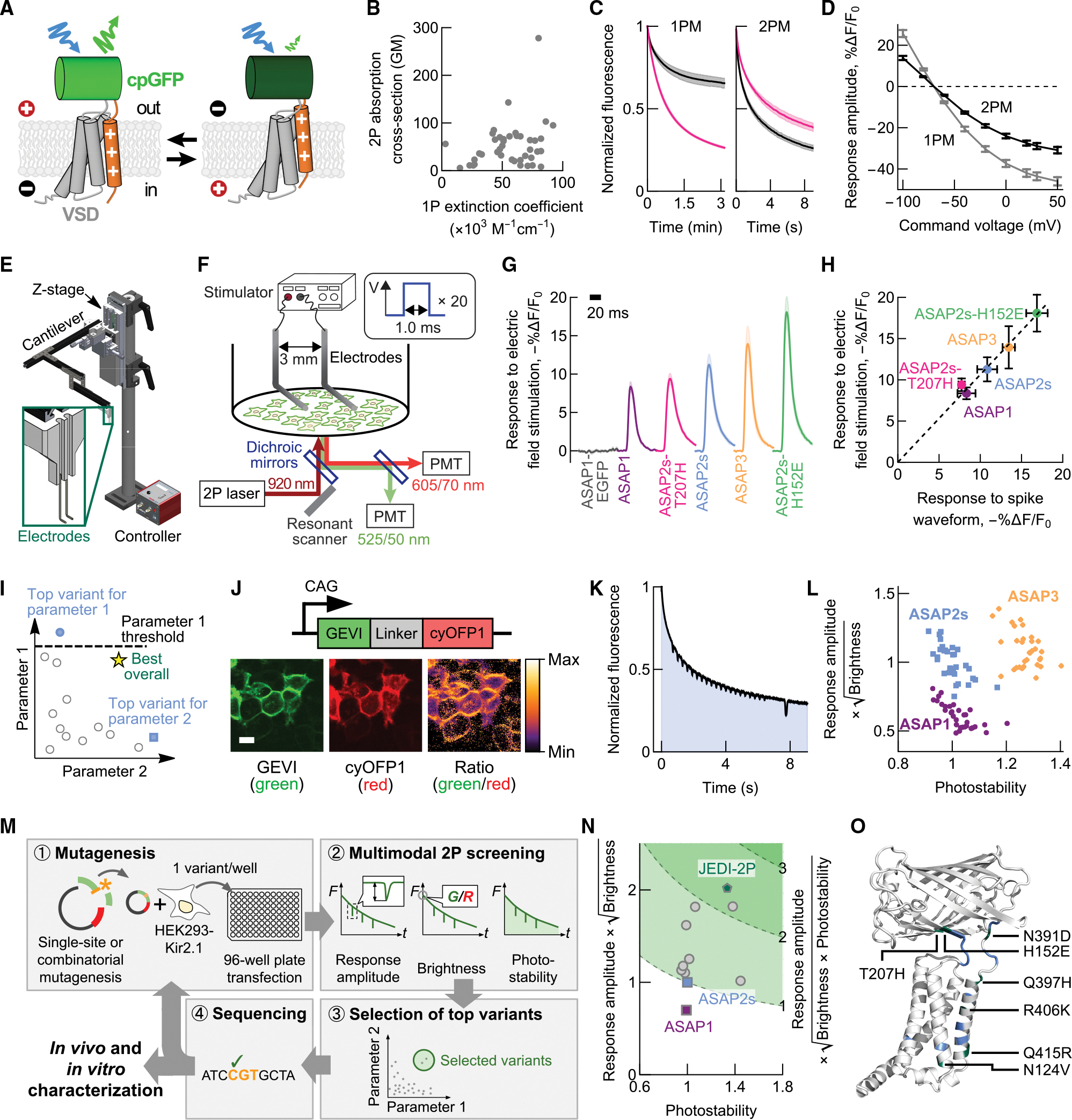
Figure 1.
Significance, design, and deployment of a multiparametric two-photon voltage indicator screening platform
(A) We optimized indicators in which a circularly permuted green fluorescent protein (cpGFP, green) is inserted into a voltage-sensing domain (VSD, gray/red). Depolarization ( right ) results in confo...
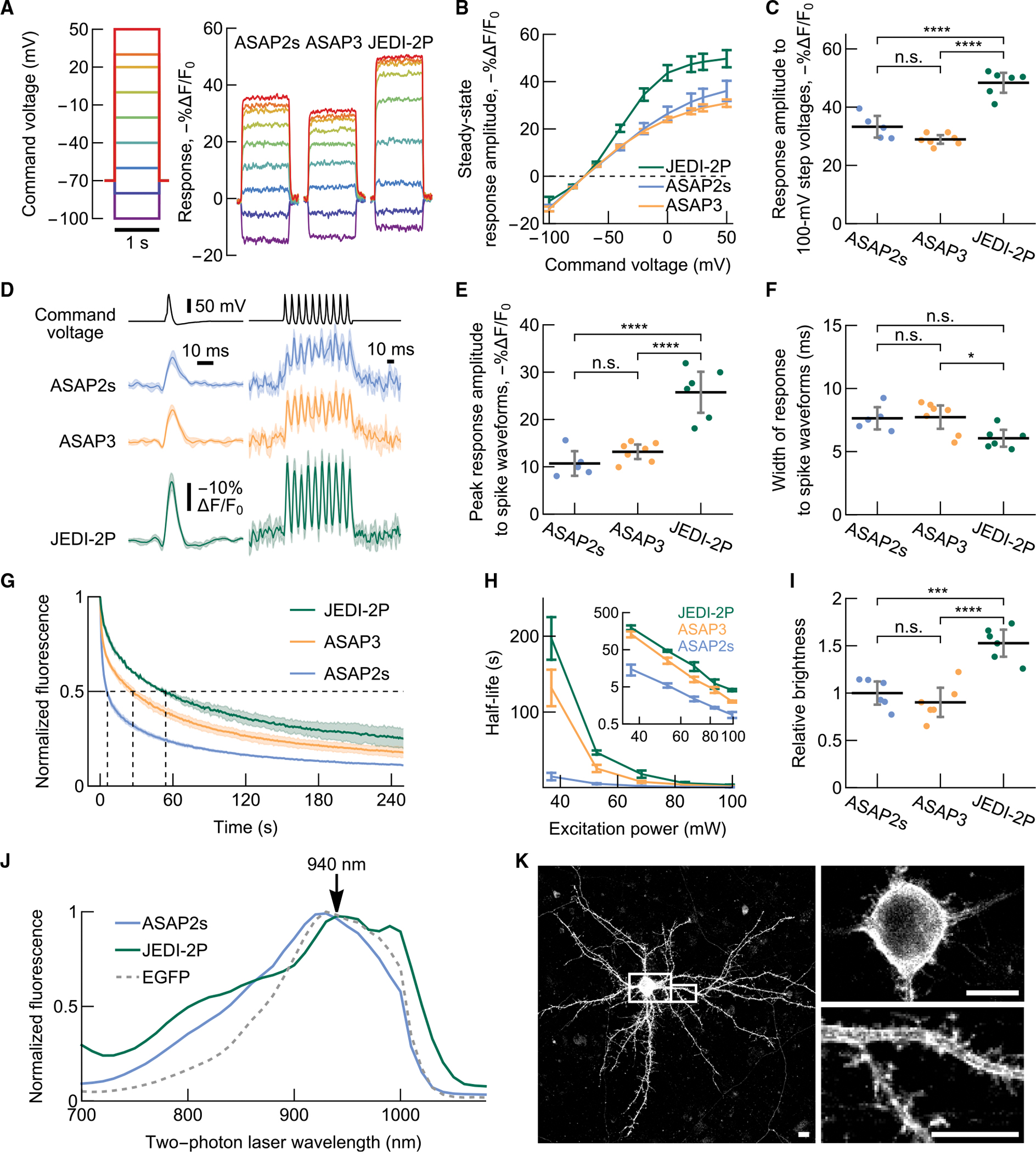
Figure 2.
JEDI-2P displays improved sensitivity, off-kinetics, brightness, and photostability under 2PM in vitro
(Au2013C) JEDI-2P produces larger steady-state responses to step depolarizations under 2PM than ASAP3 and ASAP2s. Voltage was modulated by whole-cell voltage clamp. n = 5 (ASAP2s), 7 (ASAP3), and 6 (J...
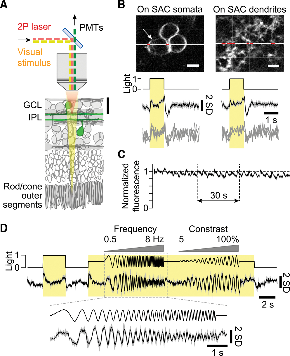
Figure 3.
JEDI-2P captures voltage responses to changes in visual stimuli frequency and contrast in isolated mouse retina
(A) Experimental setup schematic. JEDI-2P was expressed in starburst amacrine cells (SAC, green). GCL, ganglion cell layer and IPL, inner plexiform layer. Visual stimuli were presented to the photorec...
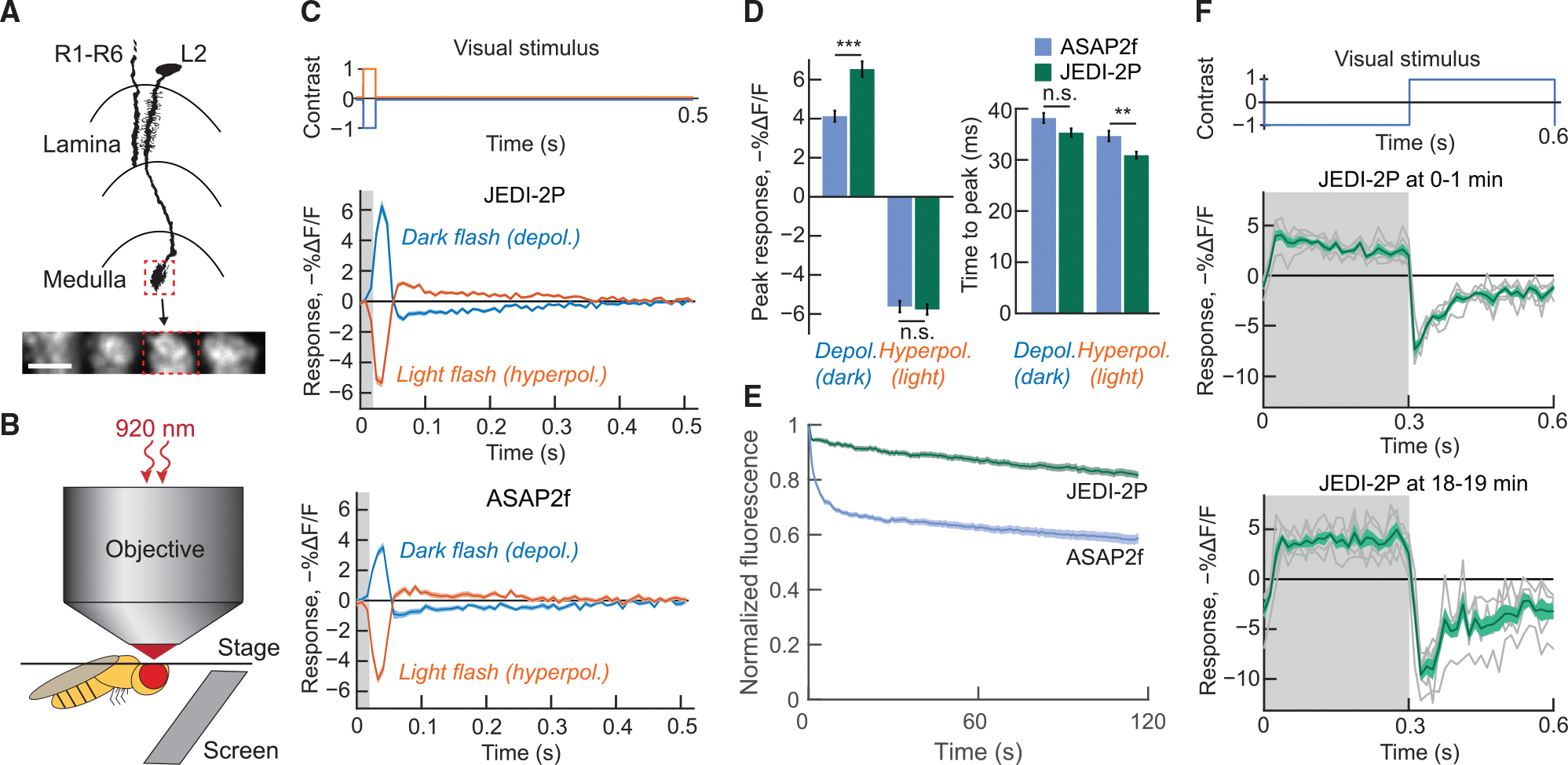
Figure 4.
JEDI-2P reports light-evoked axonal voltage transients with large response amplitude, rapid kinetics, and high photostability
(A) We imaged the axonal projections of L2 cells, non-spiking neuron postsynaptic to photoreceptors (R1u2013R6). Bottom , representative field of view showing groups of axonal termini of four neighbor...
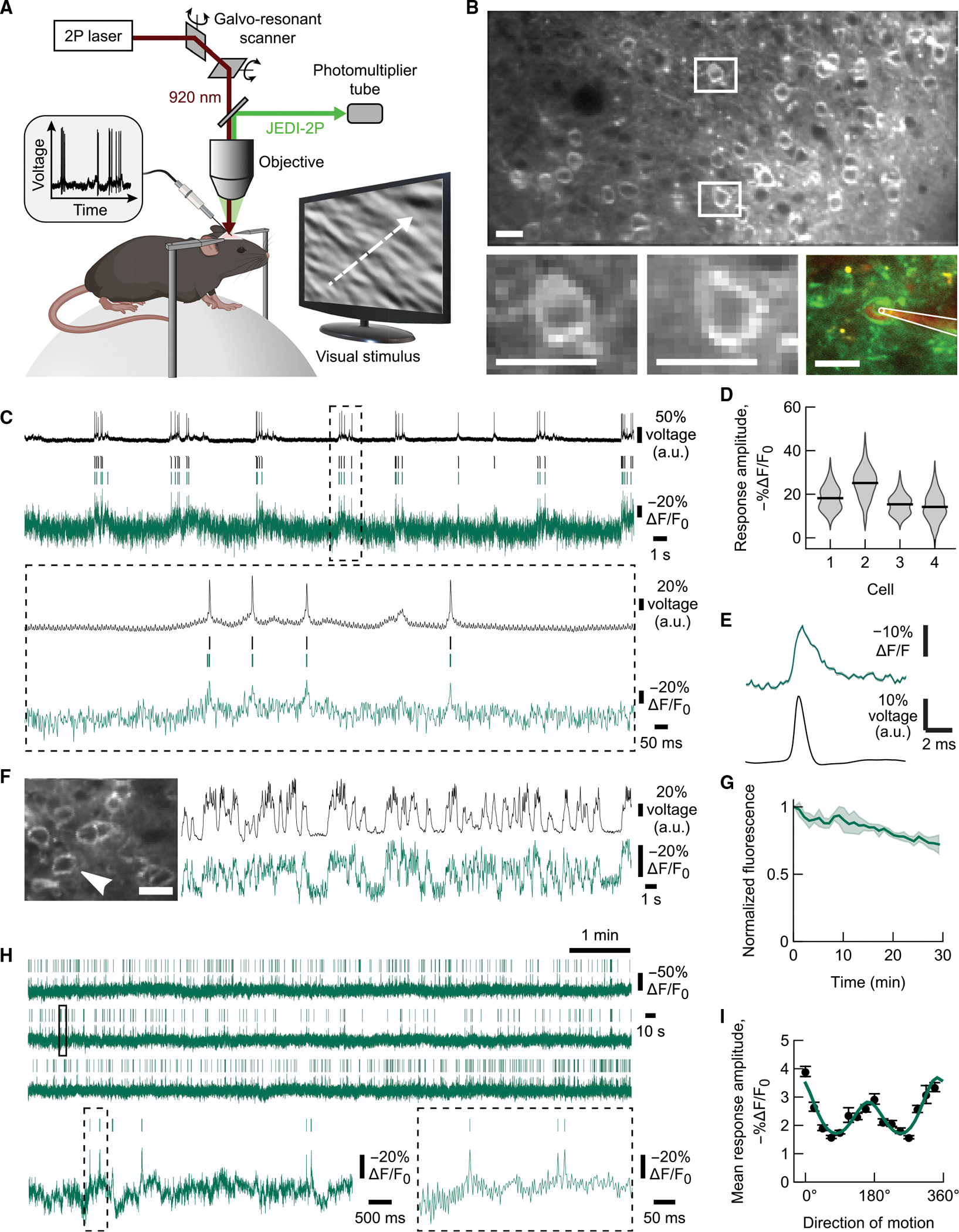
Figure 5.
JEDI-2P enables long-lasting 2P imaging of voltage dynamics in mice using resonant-scanning microscopy
(A) Experimental setup schematic. Data were collected while the mouse was presented with visual stimuli consisting of Gaussian noise with coherent orientation and motion. Mice were head fixed and free...
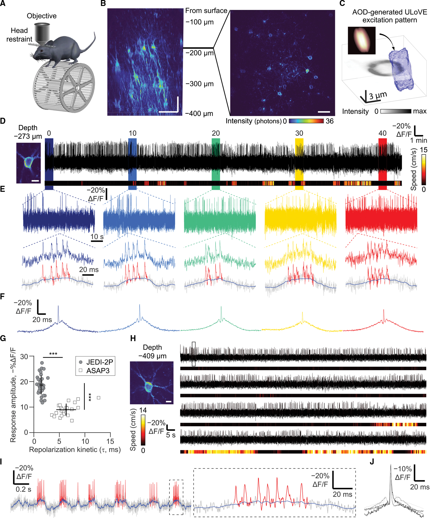
Figure 6.
Sustained high-fidelity 2P voltage recordings in cortical layers 2/3 and 5 using JEDI-2P and ULoVE microscopy
(A) During voltage recording, the head-fixed mouse is free to behave on a non-motorized wheel. (B) Representative YZ projection ( left ) and single XY plane ( right ) showing sparsely expressed JEDI-2...
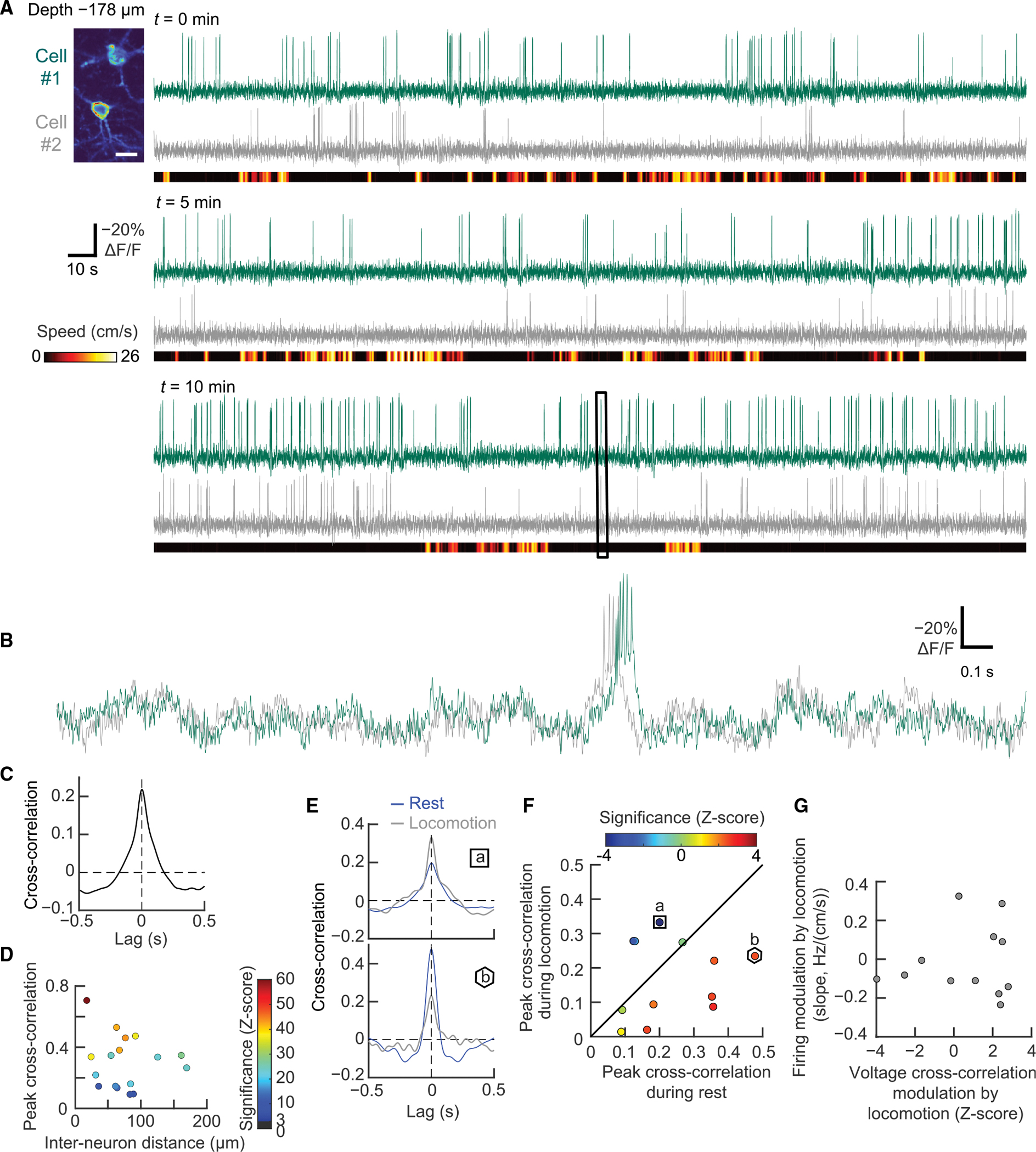
Figure 7.
ULoVE optical recording of JEDI-2P enables long-lasting recording of pairwise voltage correlations during behavior
(A) Baseline-corrected fluorescence signals from two neurons of layer 2/3 recorded simultaneously for 15.4 min. Heatmap below indicates the wheel speed. Traces were smoothed with a 1-ms Gaussian kerne...
Figure images are served from the NIH/NLM PubMed Central Open Access Subset or Europe PMC; copyright remains with the publishers and authors.
💬 Discussion
0 commentsNo comments yet. Be the first to start a discussion!
Leave a Comment